Match numbers in excel - Word и Excel - помощь в работе с программами

MATCH function

Tip: Try using the new XMATCH function, an improved version of MATCH that works in any direction and returns exact matches by default, making it easier and more convenient to use than its predecessor.

The MATCH function searches for a specified item in a range of cells, and then returns the relative position of that item in the range. For example, if the range A1:A3 contains the values 5, 25, and 38, then the formula =MATCH(25,A1:A3,0) returns the number 2, because 25 is the second item in the range.

Tip: Use MATCH instead of one of the LOOKUP functions when you need the position of an item in a range instead of the item itself. For example, you might use the MATCH function to provide a value for the row_num argument of the INDEX function.

Syntax

MATCH(lookup_value, lookup_array, [match_type])

The MATCH function syntax has the following arguments:

lookup_value Required. The value that you want to match in lookup_array. For example, when you look up someone’s number in a telephone book, you are using the person’s name as the lookup value, but the telephone number is the value you want.

The lookup_value argument can be a value (number, text, or logical value) or a cell reference to a number, text, or logical value.
lookup_array Required. The range of cells being searched.
match_type Optional. The number -1, 0, or 1. The match_type argument specifies how Excel matches lookup_value with values in lookup_array. The default value for this argument is 1.

The following table describes how the function finds values based on the setting of the match_type argument.

Match_type	Behavior
1 or omitted	MATCH finds the largest value that is less than or equal to *lookup_value. The values in the lookup_array* argument must be placed in ascending order, for example: …-2, -1, 0, 1, 2, …, A-Z, FALSE, TRUE.
0	MATCH finds the first value that is exactly equal to *lookup_value. The values in the lookup_array* argument can be in any order.
-1	MATCH finds the smallest value that is greater than or equal tolookup_value. The values in the *lookup_array* argument must be placed in descending order, for example: TRUE, FALSE, Z-A, …2, 1, 0, -1, -2, …, and so on.

MATCH returns the position of the matched value within lookup_array, not the value itself. For example, MATCH(«b»,{«a»,»b»,»c«},0) returns 2, which is the relative position of «b» within the array {«a»,»b»,»c»}.
MATCH does not distinguish between uppercase and lowercase letters when matching text values.
If MATCH is unsuccessful in finding a match, it returns the #N/A error value.
If match_type is 0 and lookup_value is a text string, you can use the wildcard characters — the question mark (?) and asterisk (*) — in the lookup_value argument. A question mark matches any single character; an asterisk matches any sequence of characters. If you want to find an actual question mark or asterisk, type a tilde (~) before the character.

Example

Copy the example data in the following table, and paste it in cell A1 of a new Excel worksheet. For formulas to show results, select them, press F2, and then press Enter. If you need to, you can adjust the column widths to see all the data.

Product	Count
Bananas	25
Oranges	38
Apples	40
Pears	41
Formula	Description	Result
=MATCH(39,B2:B5,1)	Because there is not an exact match, the position of the next lowest value (38) in the range B2:B5 is returned.	2
=MATCH(41,B2:B5,0)	The position of the value 41 in the range B2:B5.	4
=MATCH(40,B2:B5,-1)	Returns an error because the values in the range B2:B5 are not in descending order.	#N/A

Need more help?

Источник

MATCH function in Excel is used to find an exact match or the closest (less or more than the specified depending on the type of matching specified as an argument) value specified in the array or range of cells and returns the position number of the found element.

Examples of using the MATCH function in Excel

For example, we have a series of numbers from 1 to 10, written in cells B1:B10. Function =MATCH(3,B1,B10,0) will return the number 3, because the desired value is in cell B3, which is the third from the point of reference (cell B1).

This function is convenient for use in cases when it is necessary to return not the value contained in the desired cell, but its coordinate relative to the range in question. If arrays are used for constants, which can be represented as arrays of “key” — “value” elements, the FIND function returns a key value that is not explicitly specified.

For example, the array {«grapes»; «apple»; «pear»; «plum»} contains elements that can be represented as: 1 — «grapes», 2 — «apple», 3 — «pear», 4 — «plum «, Where 1, 2, 3, 4 — the keys, and the names of fruits — values. Then the function =MATCH(«apple»,{«grapes»,»apple»,»pear»,»plum»},0) returns the value 2, which is the key of the second element. The counting is performed not from 0 (zero), as it is implemented in many programming languages when working with arrays, but from 1.

MATCH function is rarely used independently. It is advisable to use it in conjunction with other functions, for example, INDEX.

Formula for finding inaccurate text matches in Excel

Example 1. Find the position of the first partial match of a string in a range of cells that store text values.

View source data table:

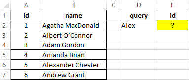
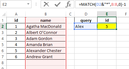
To find the position of a text string in a table, we use the following formula:

=MATCH(D2&»*»,B:B,0)-1

Argument Description:

D2 & «*» is the sought value consisting of the last name specified in cell B2 and any number of other characters (“*”);
B:B — reference to the column B: B, in which the search is performed;
0 — search for exact match.

A unit is subtracted from the obtained value to match the result with the id of the entry in the table.

Search example:

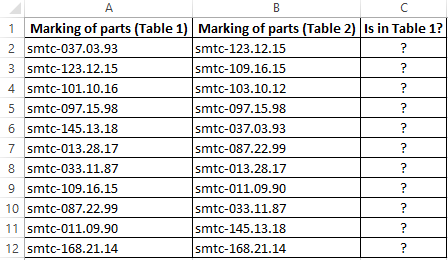
Comparison of two tables in Excel for the presence of discrepancies

Example 2. Excel stores two tables that appear to be the same at first glance. It was decided to compare one similar column of these tables for the presence of discrepancies. Implement a way to compare two cell ranges.

View of data table:

To compare the values in column B:B with the values from column A:A, use the following array formula (CTRL+SHIFT+ENTER):

MATCH function searches for a TRUE logical value in the array of logical values returned by the EXACT function (compares each element of the A2:A12 range with the value stored in cell B2 and returns an array of comparison results). If the MATCH function has found the value TRUE, the position of its first occurrence in the array will be returned. ISNA function will return FALSE if it does not accept the # N / A error value as an argument. In this case, the function IF returns the text string “is”, otherwise — “no”.

To calculate the remaining values, let us “stretch” the formula from cell C2 down to use the autocomplete function. As a result, we get:

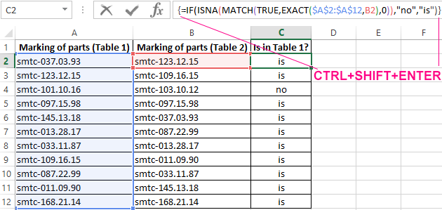
As you can see, the third elements of the lists do not match.

Finding the nearest greater knowledge in the range of Excel numbers

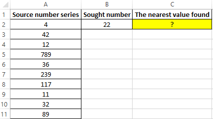
Example 3. Find the nearest smaller number to 22 in the range of numbers stored in an Excel spreadsheet column.

View source data table:

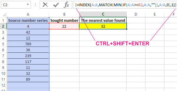
To search for the nearest larger value specified in the entire column A:A (a numerical series can be updated with new values) use the array formula (CTRL + SHIFT + ENTER):

MATCH function returns the position of the element in column A: A, which has the maximum value among the numbers that are greater than the number specified in cell B2. INDEX function returns the value stored in the found cell.

The result of the calculations:

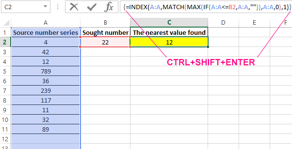
To search for the nearest smaller value, you only need to slightly change this formula and it should also be entered as an array (CTRL + SHIFT + ENTER):

Search results:

result.

Features of using the function MATCH in Excel

The function has the following syntax entry:

=MATCH(Lookup_value,Lookup_array,[Match_type])

Argument Description:

Lookup_value is a required argument that accepts textual, numeric values, as well as data of a logical and reference type, which is used as a search criterion (for comparing values or finding an exact match);
Lookup_array is a required argument that accepts data of a reference type (references to a range of cells) or an array constant in which the search for the position of an element is performed according to the criteria specified by the first argument of the function;
[Match_type] is an optional argument to fill in as a numeric value that defines how to search in a range of cells or an array. It can take the following values:

-1 — search for the smallest nearest value given by the argument is_value in an ordered or descending array or range of cells.
0 — (by default) searches for the first value in an array or range of cells (not necessarily ordered), which is exactly the same as the value passed as the first argument.
1 — Search for the largest nearest value given by the first argument in an ordered array of cells in ascending order or range.

Download examples MATCH for finding occurring values in Excel

Notes:

If a text string was passed as an argument to the Lookup_value, the MATCH function will return the position of the element in the array (if one exists) without case-sensitive characters. For example, the lines «New York» and «new york» are equivalent. To distinguish between registers, you can optionally use EXACT function.
If the search using the function in question did not return results, the error code #N/A will be returned.
If the argument [Match_type] is not explicitly specified or takes the number 0, wildcard characters can be used to search for partial match of text values (“?” Is the replacement of any single character, “*” is the replacement of any number of characters).
If the data object passed as an argument to the Lookup_array contains two or more elements corresponding to the desired value, the position of the first occurrence of such an element will be returned.

Источник

You will sometimes encounter errors while trying to MATCH or LOOKUP data in Excel if your numbers are formatted as numbers in one of your tables, and as text in another table.

While special formats are available in Excel, they are relatively rarely used and are limited. Some “numbers” such as identification numbers are more often stored as text. This is done in order to add leading zeros, hyphens and other characters to that numbers. However, if we try to MATCH or LOOKUP those numbers stored and/or formatted as text with actual numbers, we will encounter issues.

Consider the following example:

Given that number 3 in the B6 cell is stored and formatted as text, we encounter an error when we try to find a match for the number 3 in the column B.

Now consider the following example:

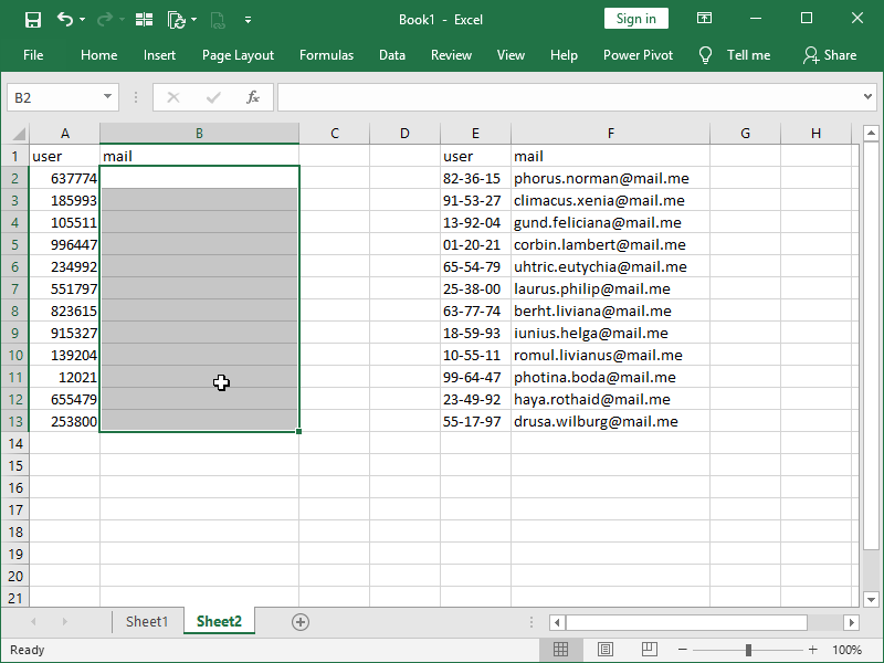
In the column A we have user numbers, formatted as numbers.

In the column E we have user numbers, formatted as text.

We have to fill the column C with the mail addresses from column F, matching user numbers from column A with those from column E.

Obviously, we will immediately encounter errors if we just plain INDEX MATCH the data:

In order to successfully match data, we should instead first take the number we are trying to match, and format it in a way our data source has it formatted. In this particular example, we can accomplish that with the help of the TEXT function:

We have successfully matched our “transformed” lookup value with the values in the column E with the help of the TEXT function.

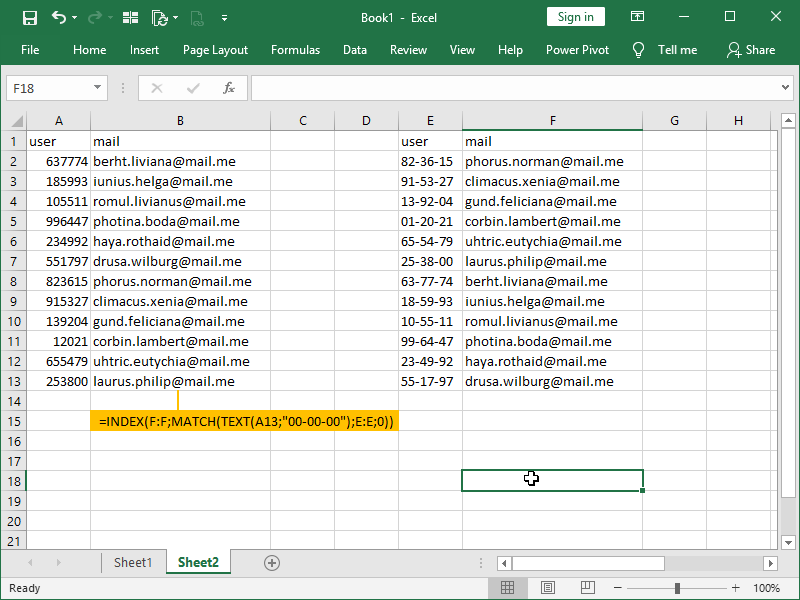
Now consider the reverse example:

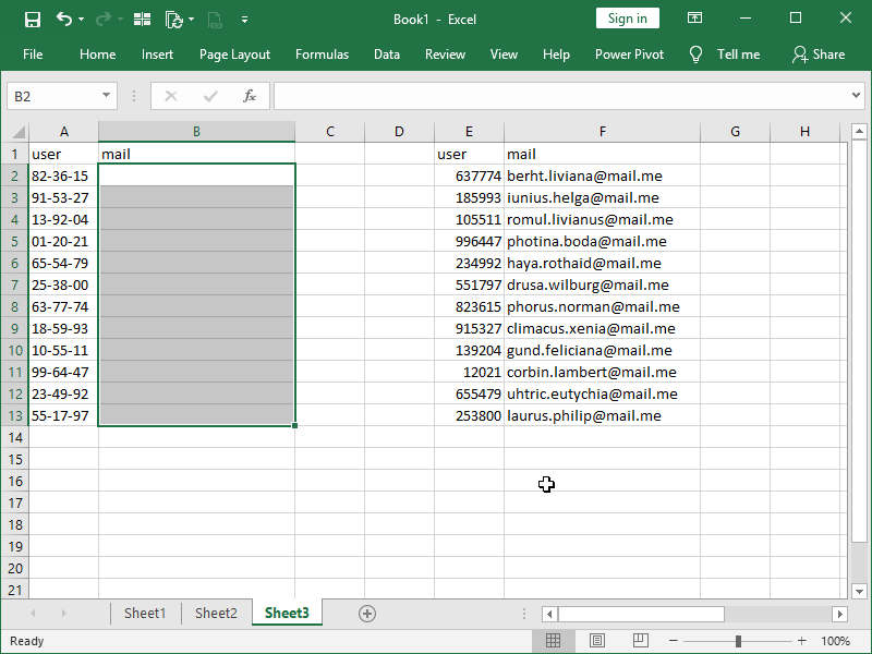
In the column A we have user numbers, formatted as text.

In the column E we have user numbers, formatted as numbers.

We have to fill the column C with the mail addresses from column F, matching user numbers from column A with those from column E.

Obviously, we will also immediately encounter errors if we just plain INDEX MATCH the data:

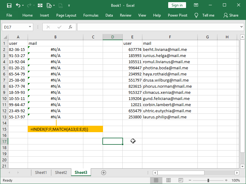
In order to successfully match data, we should instead first take the text we are trying to match, and convert that text to number, given that our data source has user codes formatted as numbers. We can accomplish that with the help of the VALUE function:

Had we’ve just been dealing with numbers formatted as text, or numbers containing leading zeros, we would have been successful. However, our numbers formatted as text also contain characters (in this case, hyphens), which the VALUE function can’t handle.

We will first have to create a new text string without text characters, and only then can we convert that new text string to number. There are several ways to do this, the basic one being with the help of the LEFT, MID and RIGHT functions:

We have successfully created a new text string that contains just digits, converted that text string to number with the help of the VALUE function, and then matched our number with the values in the column E.

In newer versions of EXCEL, we can further simplify this by using the SUBSTITUE function and generating our new text string by replacing hyphens with nothing:

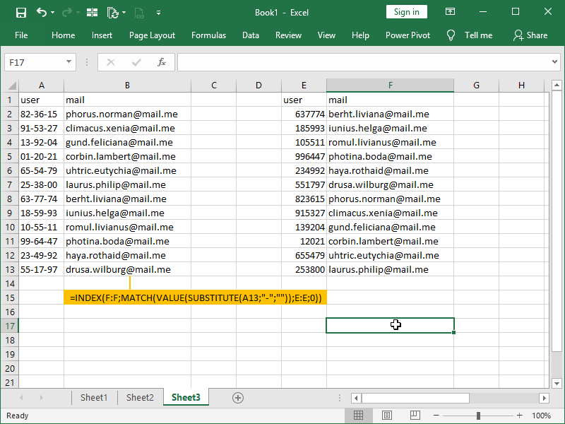
Here, we have again successfully created a new text string that contains just digits, converted that text string to number with the help of the VALUE function, and then matched our number with the values in the column E.

Dig deeper:

Lookup with unique identifiers

How to convert number to text?

How to convert text to number?

Источник

Download Article

One of Microsoft Excel’s many capabilities is the ability to compare two lists of data, identifying matches between the lists and identifying which items are found in only one list. This is useful when comparing financial records or checking to see if a particular name is in a database. You can use the MATCH function to identify and mark matching or non-matching records, or you can use conditioning formatting with the COUNTIF function. The following steps tell you how to use each to match your data.

1

Copy the data lists onto a single worksheet. Excel can work with multiple worksheets within a single workbook, or with multiple workbooks, but you’ll find comparing the lists easier if you copy their information onto a single worksheet.
2
Give each list item a unique identifier. If your two lists don’t share a common way to identify them, you may need to add an additional column to each data list that identifies that item to Excel so that it can see if an item in a given list is related to an item in the other list. The nature of this identifier will depend on the kind of data you are trying to match. You will need an identifier for each column list.
- For financial data associated with a given period, such as with tax records, this could be the description of an asset, the date the asset was acquired, or both. In some cases, an entry may be identified with a code number; however, if the same system is not used for both lists, this identifier may create matches where there are none or ignore matches that should be made.
- In some cases, you can take items from one list and combine them with items from another list to create an identifier, such as a physical asset description and the year it was purchased. To create such an identifier, you concatenate (add, combine) data from two or more cells using the ampersand (&). To combine an item description in cell F3 with a date in cell G3, separated by a space, you’d enter the formula ‘=F3&» «&G3’ in another cell in that row, such as E3. If you wanted to include only the year in the identifier (because one list uses full dates and the other uses only years), you’d include the YEAR function by entering ‘=F3&» «&YEAR(G3)’ in cell E3 instead. (Do not include the single quotes; they are there only to indicate the example.)
- Once you’ve created the formula, you can copy it into all other cells of the identifier column by selecting the cell with the formula and dragging the fill handle over the other cells of the column where you want to copy the formula. When you release your mouse button, each cell you dragged over will be populated with the formula, with the cell references adjusted to the appropriate cells in the same row.
Advertisement
3
Standardize data where possible. While the mind recognizes that «Inc.» and «Incorporated» mean the same thing, Excel doesn’t unless you have it re-format one word or the other. Likewise, you may consider values such as $11,950 and $11,999.95 as close enough to match, but Excel won’t unless you tell it to.
- You can deal with some abbreviations, such as «Co» for «Company» and «Inc» for «Incorporated by using LEFT string function to truncate the additional characters. Other abbreviations, such as «Assn» for «Association,» may best be dealt with by establishing a data entry style guide and then writing a program to look up and correct improper formats.
- For strings of numbers, such as ZIP codes where some entries include the ZIP+4 suffix and others don’t, you can again use the LEFT string function to recognize and match only the primary ZIP codes. To have Excel recognize numeric values that are close but not the same, you can use the ROUND function to round close values to the same number and match them.
- Extra spaces, such as typing two spaces between words instead of one, can be removed by using the TRIM function.
4
Create columns for the comparison formula. Just as you had to create columns for the list identifiers, you’ll need to create columns for the formula that does the comparing for you. You’ll need one column for each list.
- You’ll want to label these columns with something like «Missing?»
5
Enter the comparison formula in each cell. For the comparison formula, you’ll use the MATCH function nested inside another Excel function, ISNA.
- The formula takes the form of «=ISNA(MATCH(G3,$L$3:$L$14,FALSE))», where a cell of the identifier column of the first list is compared against each of the identifiers in the second list to see if it matches one of them. If it doesn’t match, a record is missing, and the word «TRUE» will be displayed in that cell. If it does match, the record is present, and the word «FALSE» will be displayed. (When entering the formula, do not include the enclosing quotes.)
- You can copy the formula into the remaining cells of the column the same way you copied the cell identifier formula. In this case, only the cell reference for the identifier cell changes, as putting the dollar signs in front of the row and column references for the first and last cells in the list of the second cell identifiers makes them absolute references.
- You can copy the comparison formula for the first list into the first cell of the column for the second list. You’ll then have to edit the cell references so that «G3» is replaced with the reference for the first identifier cell of the second list and «$L$3:$L$14» is replaced with the first and last identifier cell of the second list. (Leave the dollar signs and colon alone.) You can then copy this edited formula into the remaining cells in the comparison row of the second list.
6
Sort the lists to see non-matching values more easily, if necessary. If your lists are large, you may need to sort them to put all the non-matching values together. The instructions in the substeps below will convert the formulas to values to avoid recalculation errors, and if your lists are large, will avoid a long recalculation time.
- Drag your mouse over all the cells in a list to select it.
- Select Copy from the Edit menu in Excel 2003 or from the Clipboard group of the Home ribbon in Excel 2007 or 2010.
- Select Paste Special from the Edit menu in Excel 2003 or from the Paste dropdown button in the Clipboard group of Excel 2007 or 2010s Home ribbon.
- Select «Values» from the Paste As list in the Paste Special dialog box. Click OK to close the dialog.
- Select Sort from the Data menu in Excel 2003 or the Sort and Filter group of the Data ribbon in Excel 2007 or 2010.
- Select «Header row» from the «My data range has» list in the Sort By dialog, select «Missing?» (or the name you actually gave the comparison column header) and click OK.
- Repeat these steps for the other list.
7

Compare the non-matching items visually to see why they don’t match. As noted previously, Excel is designed to look for exact data matches unless you set it up to look for approximate ones. Your non-match could be as simple as an accidental transposing of letters or digits. It could also be something that requires independent verification, such as checking to see if listed assets needed to be reported in the first place.

1

Copy the data lists onto a single worksheet.
2

Decide in which list you want to highlight matching or non-matching records. If you want to highlight records in only one list, you’ll probably want to highlight the records unique to that list; that is, records that don’t match records in the other list. If you want to highlight records in both lists, you’ll want to highlight records that do match each other. For the purposes of this example, we’ll assume the first list takes up cells G3 through G14 and the second list takes up cells L3 through L14.
3

Select the items in the list you wish to highlight unique or matching items in. If you wish to highlight matching items in both lists, you’ll have to select the lists one at a time and apply the comparison formula (described in the next step) to each list.
4
Apply the appropriate comparison formula. To do this, you’ll have to access the Conditional Formatting dialog in your version of Excel. In Excel 2003, you do so by selecting Conditional Formatting from the Format menu, while in Excel 2007 and 2010, you click the Conditional Formatting button in the Styles group of the Home ribbon. Select the rule type as «Formula» and enter your formula in the Edit the Rule Description field.
- If you want to highlight records unique to the first list, the formula would be «=COUNTIF($L$3:$L$14,G3=0)», with the range of cells of the second list rendered as absolute values and the reference to the first cell of the first list as a relative value. (Don’t enter the close quotes.)
- If you want to highlight records unique to the second list, the formula would be «=COUNTIF($G$3:$G$14,L3=0)», with the range of cells of the first list rendered as absolute values and the reference to the first cell of the second list as a relative value. (Don’t enter the close quotes.)
- If you want to highlight the records in each list that are found in the other list, you’ll need two formulas, one for the first list and one for the second. The formula for the first list is «=COUNTIF($L$3:$L$14,G3>0)», while the formula for the second list is COUNTIF($G$3:$G$14,L3>0)». As noted previously, you select the first list to apply its formula and then select the second list to apply its formula.
- Apply whatever formatting you want to highlight the records being flagged. Click OK to close the dialog.

Ask a Question

200 characters left

Include your email address to get a message when this question is answered.

Submit

Video

Instead of using a cell reference with the COUNTIF conditional formatting method, you can enter a value to be searched for and flag one or more lists for instances of that value.
To simplify the comparison forms, you can create names for your list, such as «List1» and «List2.» Then, when writing the formulas, these list names can substitute for the absolute cell ranges used in the examples above.

Thanks for submitting a tip for review!

About This Article

Thanks to all authors for creating a page that has been read 107,172 times.

Is this article up to date?

Источник

Explanation

Excel supports the wildcard characters «*» and «?», and these wildcards can be used to perform partial (substring) matches in various lookup formulas. However, if you use wildcards with a number, you’ll convert the numeric value to a text value. In other words, «*»&99&»*» = «*99*» (a text string), and if you try to find a text value in a range of numbers, the match will fail.

One solution is to convert the numeric values to text with the TEXT function like this:

=MATCH("*"&E5&"*",TEXT(data,"0"),0)

This is an array formula and must be entered with Control + Shift + Enter, except in Excel 365.

This formula uses the TEXT function to transform the numbers in B5:B10 to text with the number format «0». Because we give the entire range to TEXT, we get back all values converted to text in an array, which is returned directly to the MATCH function as the array argument. With the numbers converted to text, the MATCH function can find a partial match as usual.

Note that MATCH must be configured for exact match to use wildcards, by setting the 3rd argument to zero (0) or FALSE.

Another option

Another way to to transform a number to text is to concatenate the numbers to an empty string («») with the ampersand (&) operator like this:

=MATCH("*"&E5&"*",data&"",0)

The numbers in data become text without formatting, and the result is the same as above, 7.

Источник