
MATCH function
Tip: Try using the new XMATCH function, an improved version of MATCH that works in any direction and returns exact matches by default, making it easier and more convenient to use than its predecessor.
The MATCH function searches for a specified item in a range of cells, and then returns the relative position of that item in the range. For example, if the range A1:A3 contains the values 5, 25, and 38, then the formula =MATCH(25,A1:A3,0) returns the number 2, because 25 is the second item in the range.

Tip: Use MATCH instead of one of the LOOKUP functions when you need the position of an item in a range instead of the item itself. For example, you might use the MATCH function to provide a value for the row_num argument of the INDEX function.
Syntax
MATCH(lookup_value, lookup_array, [match_type])
The MATCH function syntax has the following arguments:
-
lookup_value Required. The value that you want to match in lookup_array. For example, when you look up someone’s number in a telephone book, you are using the person’s name as the lookup value, but the telephone number is the value you want.
The lookup_value argument can be a value (number, text, or logical value) or a cell reference to a number, text, or logical value.
-
lookup_array Required. The range of cells being searched.
-
match_type Optional. The number -1, 0, or 1. The match_type argument specifies how Excel matches lookup_value with values in lookup_array. The default value for this argument is 1.
The following table describes how the function finds values based on the setting of the match_type argument.
|
Match_type |
Behavior |
|
1 or omitted |
MATCH finds the largest value that is less than or equal to lookup_value. The values in the lookup_array argument must be placed in ascending order, for example: …-2, -1, 0, 1, 2, …, A-Z, FALSE, TRUE. |
|
0 |
MATCH finds the first value that is exactly equal to lookup_value. The values in the lookup_array argument can be in any order. |
|
-1 |
MATCH finds the smallest value that is greater than or equal tolookup_value. The values in the lookup_array argument must be placed in descending order, for example: TRUE, FALSE, Z-A, …2, 1, 0, -1, -2, …, and so on. |
-
MATCH returns the position of the matched value within lookup_array, not the value itself. For example, MATCH(«b»,{«a»,»b»,»c«},0) returns 2, which is the relative position of «b» within the array {«a»,»b»,»c»}.
-
MATCH does not distinguish between uppercase and lowercase letters when matching text values.
-
If MATCH is unsuccessful in finding a match, it returns the #N/A error value.
-
If match_type is 0 and lookup_value is a text string, you can use the wildcard characters — the question mark (?) and asterisk (*) — in the lookup_value argument. A question mark matches any single character; an asterisk matches any sequence of characters. If you want to find an actual question mark or asterisk, type a tilde (~) before the character.
Example
Copy the example data in the following table, and paste it in cell A1 of a new Excel worksheet. For formulas to show results, select them, press F2, and then press Enter. If you need to, you can adjust the column widths to see all the data.
|
Product |
Count |
|
|
Bananas |
25 |
|
|
Oranges |
38 |
|
|
Apples |
40 |
|
|
Pears |
41 |
|
|
Formula |
Description |
Result |
|
=MATCH(39,B2:B5,1) |
Because there is not an exact match, the position of the next lowest value (38) in the range B2:B5 is returned. |
2 |
|
=MATCH(41,B2:B5,0) |
The position of the value 41 in the range B2:B5. |
4 |
|
=MATCH(40,B2:B5,-1) |
Returns an error because the values in the range B2:B5 are not in descending order. |
#N/A |
Need more help?
Want more options?
Explore subscription benefits, browse training courses, learn how to secure your device, and more.
Communities help you ask and answer questions, give feedback, and hear from experts with rich knowledge.
На чтение 2 мин
Функция ПОИСКПОЗ в Excel используют для поиска точной позиции искомого значения в списке или массиве данных.
Содержание
- Что возвращает функция
- Синтаксис
- Аргументы функции
- Дополнительная информация
- Примеры использования функции ПОИСКПОЗ в Excel
Что возвращает функция
Возвращает число, соответствующее позиции искомого значения.
 Больше лайфхаков в нашем Telegram Подписаться
Синтаксис
=MATCH(lookup_value, lookup_array, [match_type]) — английская версия
=ПОИСКПОЗ(искомое_значение;просматриваемый_массив;[тип_сопоставления]) — русская версия
Аргументы функции
- lookup_value (искомое_значение) — значение, с которым вы хотите сопоставить данные из массива или списка данных;
- lookup_array (просматриваемый_массив) — диапазон ячеек в котором вы осуществляете поиск искомых данных;
- [match_type] ([тип_сопоставления]) — (не обязательно) — этот аргумент определяет каким образом, будет осуществлен поиск. Допустимые значения для аргумента: «-1», «0», «1» (подробней читайте ниже).
Дополнительная информация
- Чаще всего функция MATCH используется в сочетании с функцией INDEX (ИНДЕКС);
- Подстановочные знаки могут использоваться в аргументах функции в тех случаях, когда значение поиска — текстовая строка;
- При использовании функции ПОИСКПОЗ регистр букв не учитывается;
- Функция возвращает #N/A ошибку, если искомое значение не найдено;
- Аргумент match_type (тип_сопоставления) определяет каким образом, будет осуществлен поиск:
— Если аргумент match_type (тип_сопоставления) = 0, то это критерий точного соответствия. Он возвращает первую точную позицию соответствия (или ошибку, если совпадения нет);
— Если аргумент match_type (тип_сопоставления) = 1 (по умолчанию), то в таком случае данные должны быть отсортированы в порядке возрастания для этой опции. Функция возвращает наибольшее значение, равное или меньшее значения поиска.
— Если аргумент match_type (тип_сопоставления) = -1, то в таком случае данные должны быть отсортированы в порядке убывания для этой опции. Функция возвращает наименьшее и наибольшее значения поиска.
Примеры использования функции ПОИСКПОЗ в Excel
What to Know
- The INDEX function can be used alone, but nesting the MATCH function inside it creates an advanced lookup.
- This nested function is more flexible than VLOOKUP and can yield results faster.
This article explains how to use the INDEX and MATCH functions together in all versions of Excel, including Excel 2019 and Microsoft 365.
What Are the INDEX and MATCH Functions?
INDEX and MATCH are Excel lookup functions. While they are two entirely separate functions that can be used on their own, they can also be combined to create advanced formulas.
The INDEX function returns a value or the reference to a value from within a particular selection. For example, it could be used to find the value in the second row of a data set, or in the fifth row and third column.
While INDEX could very well be used alone, nesting MATCH in the formula makes it a bit more useful. The MATCH function searches for a specified item in a range of cells and then returns the relative position of the item in the range. For example, it could be used to determine that a specific name is the third item in a list of names.
INDEX and MATCH Syntax & Arguments
This is how both functions need to be written in order for Excel to understand them:
=INDEX(array, row_num, [column_num])
- array is the range of cells that the formula will be using. It can be one or more rows and columns, such as A1:D5. It’s required.
- row_num is the row in the array from which to return a value, such as 2 or 18. It’s required unless column_num is present.
- column_num is the column in the array from which to return a value, such as 1 or 9. It’s optional.
=MATCH(lookup_value, lookup_array, [match_type])
- lookup_value is the value you want to match in lookup_array. It can be a number, text, or logical value that’s typed manually or referred to via a cell reference. This is required.
- lookup_array is the range of cells to look through. It can be a single row or a single column, such as A2:D2 or G1:G45. This is required.
- match_type can be -1, 0, or 1. It specifies how lookup_value is matched with values in lookup_array (see below). 1 is the default value if this argument is omitted.
| Which Match Type to Use | |||
|---|---|---|---|
| Match Type | What It Does | Rule | Example |
| 1 | Finds the largest value that’s less than or equal to lookup_value. | The lookup_array values must be placed in ascending order (e.g., -2, -1, 0, 1, 2; or A-Z;, or FALSE, TRUE. | lookup_value is 25 but it’s missing from lookup_array, so the position of the next smallest number, like 22, is returned instead. |
| 0 | Finds the first value that’s exactly equal to lookup_value. | The lookup_array values can be in any order. | lookup_value is 25, so it returns the position of 25. |
| -1 | Finds the smallest value that’s greater or equal to lookup_value. | The lookup_array values must be placed in descending order (e.g., 2, 1, 0, -1, -2). | lookup_value is 25 but it’s missing from lookup_array, so the position of the next largest number, like 34, is returned instead. |
Use 1 or -1 for times when you need to run an approximate lookup along a scale, like when dealing with numbers and when approximations are okay. But remember that if you don’t specify match_type, 1 will be the default, which can skew the results if you’re really wanting an exact match.
Example INDEX and MATCH Formulas
Before we look at how to combine INDEX and MATCH into one formula, we need to understand how these functions work on their own.
INDEX Examples
=INDEX(A1:B2,2,2)=INDEX(A1:B1,1)=INDEX(2:2,1)=INDEX(B1:B2,1)
In this first example, there are four INDEX formulas we can use to get different values:
- =INDEX(A1:B2,2,2) looks through A1:B2 to find the value in the second column and second row, which is Stacy.
- =INDEX(A1:B1,1) looks through A1:B1 to find the value in the first column, which is Jon.
- =INDEX(2:2,1) looks through everything in the second row to locate the value in the first column, which is Tim.
- =INDEX(B1:B2,1) looks through B1:B2 to locate the value in the first row, which is Amy.
MATCH Examples
=MATCH("Stacy",A2:D2,0)=MATCH(14,D1:D2)=MATCH(14,D1:D2,-1)=MATCH(13,A1:D1,0)
Here are four easy examples of the MATCH function:
- =MATCH(«Stacy»,A2:D2,0) is searching for Stacy in the range A2:D2 and returns 3 as the result.
- =MATCH(14,D1:D2) is searching for 14 in the range D1:D2, but since it’s not found in the table, MATCH finds the next largest value that’s less than or equal to 14, which in this case is 13, which is in position 1 of lookup_array.
- =MATCH(14,D1:D2,-1) is identical to the formula above it, but since the array isn’t in descending order like -1 requires, we get an error.
- =MATCH(13,A1:D1,0) is looking for 13 in the first row of the sheet, which returns 4 since it’s the fourth item in this array.
INDEX-MATCH Examples
Here are two examples where we can combine INDEX and MATCH in one formula:
Find Cell Reference in Table
=INDEX(B2:B5,MATCH(F1,A2:A5))
This example is nesting the MATCH formula within the INDEX formula. The goal is to identify the item color using the item number.
If you look at the image, you can see in the «Separated» rows how the formulas would be written on their own, but since we’re nesting them, this is what’s happening:
- MATCH(F1,A2:A5) is looking for the F1 value (8795) in the data set A2:A5. If we count down the column, we can see it’s 2, so that’s what the MATCH function just figured out.
- The INDEX array is B2:B5 since we’re ultimately looking for the value in that column.
- The INDEX function could now be rewritten like this since 2 is what MATCH found: INDEX(B2:B5, 2, [column_num]).
- Since column_num is optional, we can remove that to be left with this: INDEX(B2:B5,2).
- So now, this is like a normal INDEX formula where we’re finding the value of the second item in B2:B5, which is red.
Lookup By Row and Column Headings
=INDEX(B2:E13,MATCH(G1,A2:A13,0),MATCH(G2,B1:E1,0))
In this example of MATCH and INDEX, we’re doing a two-way lookup. The idea is to see how much money we made off of Green items in May. This is really similar to the example above, but an extra MATCH formula is nested in INDEX.
- MATCH(G1,A2:A13,0) is the first item solved in this formula. It’s looking for G1 (the word «May») in A2:A13 to get a particular value. We don’t see it here, but it’s 5.
- MATCH(G2,B1:E1,0) is the second MATCH formula, and it’s really similar to the first but is instead looking for G2 (the word «Green») in the column headings at B1:E1. This one resolves to 3.
- We can now rewrite the INDEX formula like this to visualize what’s happening: =INDEX(B2:E13,5,3). This is looking in the whole table, B2:E13, for the fifth row and third column, which returns $180.
MATCH and INDEX Rules
There are several things to keep in mind when writing formulas with these functions:
- MATCH isn’t case sensitive, so uppercase and lowercase letters are treated the same when matching text values.
- MATCH returns #N/A for multiple reasons: if match_type is 0 and lookup_value isn’t found if match_type is -1 and lookup_array isn’t in descending order, if match_type is 1 and lookup_array isn’t in ascending order, and if lookup_array isn’t a single row or column.
- You can use a wildcard character in the lookup_value argument if match_type is 0 and lookup_value is a text string. A question mark matches any single character and an asterisk matches any sequence of characters (e.g., =MATCH(«Jo*»,1:1,0)). To use MATCH to find an actual question mark or asterisk, type ~ first.
- INDEX returns #REF! if row_num and column_num don’t point to a cell within the array.
Related Excel Functions
The MATCH function is similar to LOOKUP, but MATCH returns the position of the item instead of the item itself.
VLOOKUP is another lookup function you can use in Excel, but unlike MATCH which requires INDEX for advanced lookups, VLOOKUP formulas only need that one function.
Thanks for letting us know!
Get the Latest Tech News Delivered Every Day
Subscribe
| английском | русском |
|---|---|
| MATCH |
ПОИСКПОЗ |
Описание
Функция ПОИСКПОЗ выполняет поиск указанного элемента в диапазоне (Диапазон. Две или более ячеек листа. Ячейки диапазона могут быть как смежными, так и несмежными.) ячеек и возвращает относительную позицию этого элемента в диапазоне. Например, если диапазон A1:A3 содержит значения 5, 25 и 38, то формула
=ПОИСКПОЗ(25;A1:A3;0)
возвращает значение 2, поскольку элемент 25 является вторым в диапазоне.
Функцией ПОИСКПОЗ следует пользоваться вместо одной из функций ПРОСМОТР, когда требуется найти позицию элемента в диапазоне, а не сам элемент. Например, функцию ПОИСКПОЗ можно использовать для передачи значения аргумента номер_строки функции ИНДЕКС.
Дополнительная информация (источник)
Возвращает относительное положение элемента в массиве или диапазоне ячеек
Возвращает ссылку на отдельную ячейку листа в виде текста
Ищет значение в первом столбце массива и возвращает значение из ячейки в найденной строке и указанном столбце
Выбирает значение из списка значений
Создает ссылку, открывающую документ, который находится на сервере сети, в интрасети или в Интернете
Выполняет поиск в первой строке массива и возвращает значение указанной ячейки
Возвращает ссылку, заданную текстовым значением
Извлекает данные реального времени из программ, поддерживающих автоматизацию COM
Использует индекс для выбора значения из ссылки или массива
Возвращает количество областей в ссылке
Возвращают данные, хранящиеся в отчете сводной таблицы
Ищет значения в векторе или массиве
Выполняет поиск в диапазоне или массиве и возвращает элемент, соответствующий первому совпадению Если совпадения не существует, то она может вернуть наиболее близкое (приблизительное) совпадение
Возвращает смещение ссылки относительно заданной ссылки
Сортировка содержимого диапазона или массива
Сортировка содержимого диапазона или массива на основе значений в соответствующем диапазоне или массиве
Возвращает номер столбца, на который указывает ссылка
Возвращает номер строки, определяемой ссылкой
Возвращает транспонированный массив
Возвращает список уникальных значений в списке или диапазоне
Возвращает формулу в заданной ссылке в виде текста
Фильтрация диапазона данных на основе за определенных критериев
Возвращает количество столбцов в ссылке
Возвращает количество строк в ссылке
Функция
ПОИСКПОЗ(
)
, английский вариант MATCH(),
возвращает позицию значения в диапазоне ячеек. Например, если в ячейке
А10
содержится значение «яблоки», то формула
=ПОИСКПОЗ («яблоки»;A9:A20;0)
вернет 2, т.е. искомое значение «яблоки» содержится во второй ячейке диапазона
A9:A20
:
А9
— первая ячейка (предполагается, что в ней не содержится значение «яблоки»),
А10
— вторая,
А11
— третья и т.д. (подсчет позиции производится от верхней ячейки)
.
Функция
ПОИСКПОЗ()
возвращает позицию искомого значения, а не само значение. Например:
ПОИСКПОЗ(«б»;{«а»;»б»;»в»;»б»};0)
возвращает число 2 — относительную позицию буквы «б» в массиве {«а»;»б»;»в»;»б»}. Позиция второй буквы «б» будет проигнорирована, функция вернет позицию только первой буквы. О том как вернуть ВСЕ позиции искомого значения читайте ниже в разделе
Поиск позиций ВСЕХ текстовых значений, удовлетворяющих критерию
.
Синтаксис функции
ПОИСКПОЗ
(
искомое_значение
;
просматриваемый_массив
; тип_сопоставления)
Искомое_значение
— значение, используемое при поиске значения в
просматриваемом_массиве
.
Искомое_значение
может быть значением (числом, текстом или логическим значением (ЛОЖЬ или ИСТИНА)) или ссылкой на ячейку, содержащую число, текст или логическое значение.
Просматриваемый_массив
— непрерывный диапазон ячеек, возможно, содержащих искомые значения.
Просматриваемый_массив
может быть только одностолбцовым диапазоном ячеек, например
А9:А20
или диапазоном, расположенным в одной строке, например,
А2:Е2
. Таким образом формула
=ПОИСКПОЗ(«слива»;A30:B33;0)
работать не будет (выдаст ошибку #Н/Д), так как
Просматриваемый_массив
представляет собой диапазон ячеек размещенный одновременно в нескольких столбцах и нескольких ячейках.
Тип_сопоставления
— число -1, 0 или 1.
Тип_сопоставления
указывает, как MS EXCEL сопоставляет
искомое_значение
со значениями в аргументе
просматриваемый_массив.
-
Если
тип_сопоставления
равен 0, то функция
ПОИСКПОЗ()
находит первое значение, которое в
точности
равно аргументу
искомое_значение
.
Просматриваемый_массив
может быть не упорядочен. -
Если тип_сопоставления равен 1, то функция
ПОИСКПОЗ()
находит наибольшее значение, которое меньше либо равно, чем
искомое_значение
.
Просматриваемый_массив
должен быть упорядочен по возрастанию: …, -2, -1, 0, 1, 2, …, A-Z, ЛОЖЬ, ИСТИНА. Если
тип_сопоставления
опущен, то предполагается, что он равен 1. -
Если
тип_сопоставления
равен -1, то функция
ПОИСКПОЗ()
находит наименьшее значение, которое больше либо равно чем
искомое_значение
.
Просматриваемый_массив
должен быть упорядочен по убыванию: ИСТИНА, ЛОЖЬ, Z-A, …, 2, 1, 0, -1, -2, …, и так далее.
Функция
ПОИСКПОЗ()
не различает
РеГИстры
при сопоставлении текстов.
Если функция
ПОИСКПОЗ()
не находит соответствующего значения, то возвращается значение ошибки #Н/Д.
Поиск позиции в массивах с текстовыми значениями
Произведем поиск позиции в НЕ сортированном списке текстовых значений (диапазон
B7:B13
)
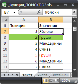
Столбец
Позиция
приведен для наглядности и не влияет на вычисления.
Формула для поиска позиции значения
Груши:
=ПОИСКПОЗ(«груши»;B7:B13;0)
Формула находит первое значение сверху и выводит его позицию в диапазоне, второе значение
Груши
учтено не будет.
Чтобы найти номер строки, а не позиции в искомом диапазоне, можно записать следующую формулу:
=ПОИСКПОЗ(«груши»;B7:B13;0)+СТРОКА($B$6)
Если искомое значение не обнаружено в списке, то будет возвращено значение ошибки #Н/Д. Например, формула
=ПОИСКПОЗ(«грейпфрут»;B7:B13;0)
вернет ошибку, т.к. значения «грейпфрут» в диапазоне ячеек
B7:B13
нет.
В
файле примера
можно найти применение функции при поиске в горизонтальном массиве.
Поиск позиции в массиве констант
Поиск позиции можно производить не только в диапазонах ячеек, но и в
массивах констант
. Например, формула
=ПОИСКПОЗ(«груши»;{«яблоки»;»ГРУШИ»;»мандарины»};0)
вернет значение 2.
Поиск позиции с использованием подстановочных знаков
Если искомое значение точно не известно, то с помощью
подстановочных знаков
можно задать поиск по шаблону, т.е. искомое_значение может содержать знаки шаблона: звездочку (*) и знак вопроса (?). Звездочка соответствует любой последовательности знаков, знак вопроса соответствует любому одиночному знаку.
Предположим, что имеется перечень товаров и мы не знаем точно как записана товарная позиция относящаяся к яблокам:
яблоки
или
яблоко
.
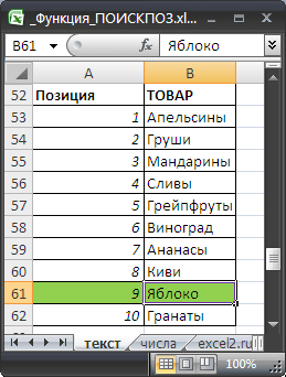
В качестве критерия можно задать
«яблок*»
и формула
=ПОИСКПОЗ(«яблок*»;B53:B62;0)
вернет позицию текстового значения, начинающегося со слова
яблок
(если она есть в списке).
Подстановочные знаки
следует использовать только для поиска позиции текстовых значений и
Типом сопоставления
= 0 (третий аргумент функции).
Поиск позиций ВСЕХ текстовых значений, удовлетворяющих критерию
Функция
ПОИСКПОЗ()
возвращает только одно значение. Если в списке присутствует несколько значений, удовлетворяющих критерию, то эта функция не поможет.
Рассмотрим список с
повторяющимися
значениями в диапазоне
B66:B72
. Найдем все позиции значения
Груши
.
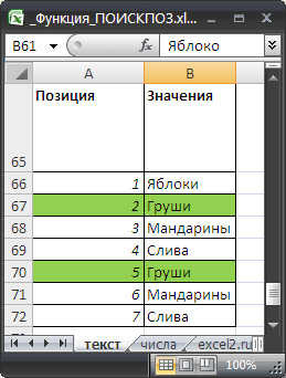
Значение
Груши
находятся в позициях 2 и 5 списка. С помощью
формулы массива
=(«груши»=$B$66:$B$72)*(СТРОКА($B$66:$B$72)-СТРОКА($D$65))
можно найти все эти позиции. Для этого необходимо выделить несколько ячеек (расположенных вертикально), в
Строке формул
ввести вышеуказанную формулу и нажать
CTRL+SHIFT+ENTER
. В позициях, в которых есть значение
Груши
будет выведено соответствующее значение позиции, в остальных ячейках быдет выведен 0.
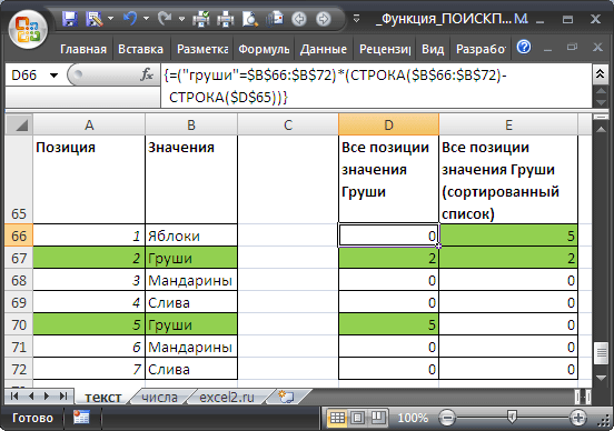
C помощью другой
формулы массива
=НАИБОЛЬШИЙ((«груши»=$B$66:$B$72)*(СТРОКА($B$66:$B$72)-СТРОКА($D$65));СТРОКА()-СТРОКА($D$65))
можно отсортировать найденные позиции, чтобы номера найденных позиций отображались в первых ячейках (см.
файл примера
).
Поиск позиции в массивах с Числами
1. Произведем поиск позиции в НЕ сортированном списке числовых значений (диапазон
B8:B14
)
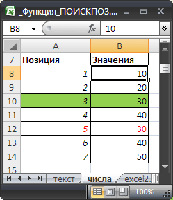
Столбец
Позиция
приведен для наглядности и не влияет на вычисления.
Найдем позицию значения 30 с помощью формулы
=ПОИСКПОЗ(30;B8:B14;0)
Формула ищет
точное
значение 30. Если в списке его нет, то будет возвращена ошибка #Н/Д.
2. Произведем поиск позиции в
отсортированном
по возрастанию списке числовых значений (диапазон
B31:B37
)
Сортированные списки позволяют искать не только точные значения (их позицию), но и позицию
ближайшего
значения. Например, в списке на картинке ниже нет значения 45, но можно найти позицию наибольшего значения, которое меньше либо равно, чем искомое значение, т.е. позицию значения 40.
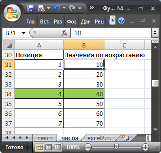
Это можно сделать с помощью формулы
=ПОИСКПОЗ(45;B31:B37;1)
Обратите внимание, что тип сопоставления =1 (третий аргумент функции).
3. Поиск позиции в списке
отсортированном
по убыванию выполняется аналогично, но с типом сопоставления = -1. В этом случае функция
ПОИСКПОЗ()
находит наименьшее значение, которое больше либо равно чем искомое значение.
Функции ПОИСКПОЗ() и ИНДЕКС()
Функции
ПОИСКПОЗ()
и
ИНДЕКС()
часто используются вместе, т.к. позволяют по найденной позиции в одном диапазоне вывести соответствующее значение из другого диапазона. Рассмотрим пример.
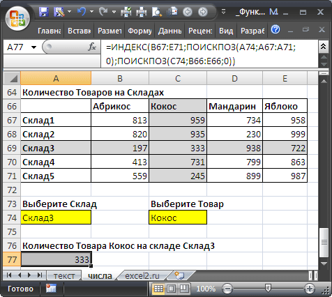
Найдем количество заданного товара на определенном складе. Для этого используем формулу
=ИНДЕКС(B67:E71;ПОИСКПОЗ(A74;A67:A71;0);ПОИСКПОЗ(C74;B66:E66;0))
В
файле примера
, соответствующий столбец и строка выделены с помощью
Условного форматирования
.
СОВЕТ:
Подробнее о поиске позиций можно прочитать в соответствующем разделе сайта:
Поиск позиции
.
С помощью функций
ПОИСКПОЗ()
и
ИНДЕКС()
можно заменить функцию
ВПР()
, об этом читайте в статье о
функции ВПР()
.
The MATCH function is used to determine the position of a value in a range or array. For example, in the screenshot above, the formula in cell E6 is configured to get the position of the value in cell D6. The MATCH function returns 5 because the lookup value («peach») is in the 5th position in the range B6:B14:
=MATCH(D6,B6:B14,0) // returns 5
The MATCH function can perform exact and approximate matches and supports wildcards (* ?) for partial matches. There are 3 separate match modes (set by the match_type argument), as described below.
Note: the MATCH function will always return the first match. If you need to return the last match (reverse search) see the XMATCH function. If you want to return all matches, see the FILTER function.
MATCH only supports one-dimensional arrays or ranges, either vertical or horizontal. However, you can use MATCH to locate values in a two-dimensional range or table by giving MATCH the single column (or row) that contains the lookup value. You can even use MATCH twice in a single formula to find a matching row and column at the same time.
Frequently, the MATCH function is combined with the INDEX function to retrieve a value at a certain (matched) position. In other words, MATCH figures out the position, and INDEX returns the value at that position. For a detailed overview with simple examples, see How to use INDEX and MATCH.
Match type information
Match type is optional. If not provided, match_type defaults to 1 (exact or next smallest). When match_type is 1 or -1, it is sometimes referred to as an «approximate match». However, keep in mind that MATCH will always perform an exact match when possible, as noted in the table below:
| Match type | Behavior | Details |
|---|---|---|
| 1 | Approximate | MATCH finds the largest value less than or equal to the lookup value. The lookup array must be sorted in ascending order. |
| 0 | Exact | MATCH finds the first value equal to the lookup value. The lookup array does not need to be sorted. |
| -1 | Approximate | MATCH finds the smallest value greater than or equal to the lookup value. The lookup array must be sorted in descending order. |
| (omitted) | Approximate | When match_type is omitted, it defaults to 1 with behavior as explained above. |
Caution: Be sure to set match_type to zero (0) if you need an exact match. The default setting of 1 can cause MATCH to return results that look normal but are in fact incorrect. Explicitly providing a value for match_type, is a good reminder of what behavior is expected.
Exact match
When match_type is zero (0), MATCH performs an exact match only. In the example below, the formula in E3 is:
=MATCH(E2,B3:B11,0) // returns 4

In the formula above, the lookup value comes from cell E2. If the lookup value is hardcoded into the formula, it must be enclosed in double quotes («»), since it is a text value:
=MATCH("Mars",B3:B11,0)
Note: MATCH is not case-sensitive, so «Mars» and «mars» will both return 4.
Approximate match
When match_type is set to 1, MATCH will perform an approximate match on values sorted A-Z, finding the largest value less than or equal to the lookup value. In the example shown below, the formula in E3 is:
=MATCH(E2,B3:B11,1) // returns 5

Wildcard match
When match_type is set to zero (0), MATCH can use wildcards. In the example shown below, the formula in E3 is:
=MATCH(E2,B3:B11,0) // returns 6
This is equivalent to:
=MATCH("pq*",B3:B11,0)

INDEX and MATCH
The MATCH function is commonly used together with the INDEX function. The resulting formula is called «INDEX and MATCH». For example, in the screen below, INDEX and MATCH are used to return the cost of a code entered in cell F4. The formula in F5 is:
=INDEX(C5:C12,MATCH(F4,B5:B12,0)) // returns 150

In this example, MATCH is set up to perform an exact match. The MATCH function locates the code ABX-075 and returns its position (7) directly to the INDEX function as the row number. The INDEX function then returns the 7th value from the range C5:C12 as a final result. The formula is solved like this:
=INDEX(C5:C12,MATCH(F4,B5:B12,0))
=INDEX(C5:C12,7)
=150
See below for more examples of the MATCH function. For an overview of how to use INDEX and MATCH with many examples, see: How to use INDEX and MATCH.
Case-sensitive match
The MATCH function is not case-sensitive. However, MATCH can be configured to perform a case-sensitive match when combined with the EXACT function in a generic formula like this:
=MATCH(TRUE,EXACT(lookup_value,array),0))
The EXACT function compares every value in array with the lookup_value in a case-sensitive manner. This formula is explained with an INDEX and MATCH example here.
Notes
- MATCH is not case-sensitive.
- MATCH returns the #N/A error if no match is found.
- MATCH only works with text up to 255 characters in length.
- In case of duplicates, MATCH returns the first match.
- If match_type is -1 or 1, the lookup_array must be sorted as noted above.
- If match_type is 0, the lookup_value can contain the wildcards.
- The MATCH function is frequently used together with the INDEX function.