Match more than one excel - Word и Excel - помощь в работе с программами

Содержание

How to use INDEX and MATCH
Summary
The INDEX Function
The MATCH function
INDEX and MATCH together
Two-way lookup with INDEX and MATCH
Left lookup
Case-sensitive lookup
Closest match
Multiple criteria lookup
More examples of INDEX + MATCH
INDEX and MATCH with multiple criteria
Related functions
Summary
Generic formula
Explanation
Array visualization
Non-array version
MATCH
Syntax
Example

How to use INDEX and MATCH

Summary

INDEX and MATCH is the most popular tool in Excel for performing more advanced lookups. This is because INDEX and MATCH are incredibly flexible – you can do horizontal and vertical lookups, 2-way lookups, left lookups, case-sensitive lookups, and even lookups based on multiple criteria. If you want to improve your Excel skills, INDEX and MATCH should be on your list. See below for many examples.

This article explains in simple terms how to use INDEX and MATCH together to perform lookups. It takes a step-by-step approach, first explaining INDEX, then MATCH, then showing you how to combine the two functions together to create a dynamic two-way lookup. There are more advanced examples further down the page.

The INDEX Function

The INDEX function in Excel is fantastically flexible and powerful, and you’ll find it in a huge number of Excel formulas, especially advanced formulas. But what does INDEX actually do? In a nutshell, INDEX retrieves the value at a given location in a range. For example, let’s say you have a table of planets in our solar system (see below), and you want to get the name of the 4th planet, Mars, with a formula. You can use INDEX like this:

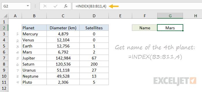
INDEX returns the value in the 4th row of the range.

What if you want to get the diameter of Mars with INDEX? In that case, we can supply both a row number and a column number, and provide a larger range. The INDEX formula below uses the full range of data in B3:D11, with a row number of 4 and column number of 2:

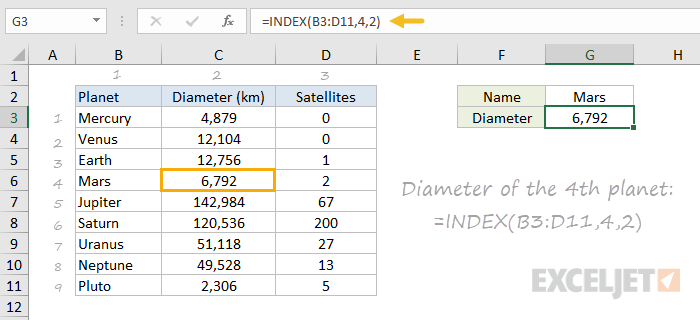
INDEX retrieves the value at row 4, column 2.

To summarize, INDEX gets a value at a given location in a range of cells based on numeric position. When the range is one-dimensional, you only need to supply a row number. When the range is two-dimensional, you’ll need to supply both the row and column number.

At this point, you may be thinking «So what? How often do you actually know the position of something in a spreadsheet?»

Exactly right. We need a way to locate the position of things we’re looking for.

Enter the MATCH function.

The MATCH function

The MATCH function is designed for one purpose: find the position of an item in a range. For example, we can use MATCH to get the position of the word «peach» in this list of fruits like this:

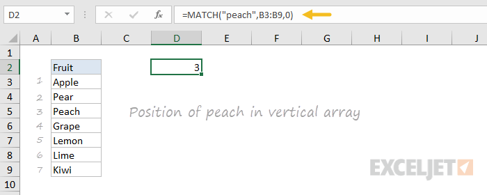
MATCH returns 3, since «Peach» is the 3rd item. MATCH is not case-sensitive.

MATCH doesn’t care if a range is horizontal or vertical, as you can see below:

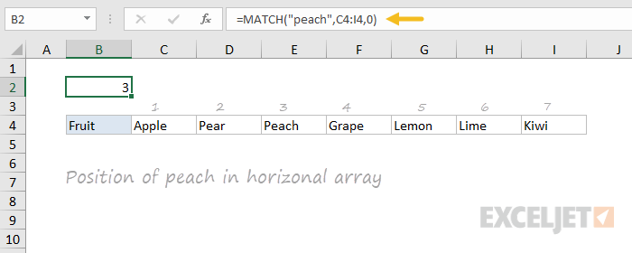
Same result with a horizontal range, MATCH returns 3.

Important: The last argument in the MATCH function is match_type. Match_type is important and controls whether matching is exact or approximate. In many cases you will want to use zero (0) to force exact match behavior. Match_type defaults to 1, which means approximate match, so it’s important to provide a value. See the MATCH page for more details.

INDEX and MATCH together

Now that we’ve covered the basics of INDEX and MATCH, how do we combine the two functions in a single formula? Consider the data below, a table showing a list of salespeople and monthly sales numbers for three months: January, February, and March.

Let’s say we want to write a formula that returns the sales number for February for a given salesperson. From the discussion above, we know we can give INDEX a row and column number to retrieve a value. For example, to return the February sales number for Frantz, we provide the range C3:E11 with a row 5 and column 2:

But we obviously don’t want to hardcode numbers. Instead, we want a dynamic lookup.

How will we do that? The MATCH function of course. MATCH will work perfectly for finding the positions we need. Working one step at a time, let’s leave the column hardcoded as 2 and make the row number dynamic. Here’s the revised formula, with the MATCH function nested inside INDEX in place of 5:

Taking things one step further, we’ll use the value from H2 in MATCH:

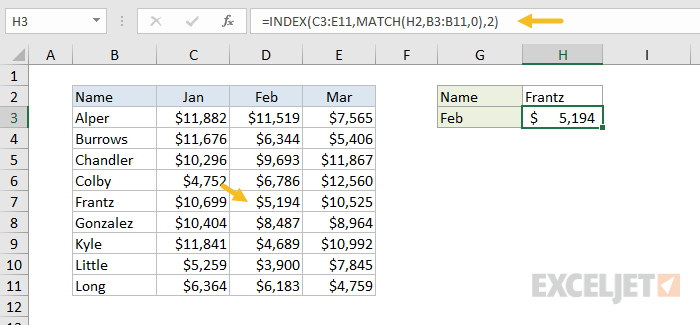
MATCH finds «Frantz» and returns 5 to INDEX for row.

INDEX needs numeric positions.
MATCH finds those positions.
MATCH is nested inside INDEX.

Let’s now tackle the column number.

Two-way lookup with INDEX and MATCH

Above, we used the MATCH function to find the row number dynamically, but hardcoded the column number. How can we make the formula fully dynamic, so we can return sales for any given salesperson in any given month? The trick is to use MATCH twice – once to get a row position, and once to get a column position.

From the examples above, we know MATCH works fine with both horizontal and vertical arrays. That means we can easily find the position of a given month with MATCH. For example, this formula returns the position of March, which is 3:

But of course we don’t want to hardcode any values, so let’s update the worksheet to allow the input of a month name, and use MATCH to find the column number we need. The screen below shows the result:

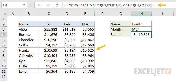
A fully dynamic, two-way lookup with INDEX and MATCH.

The first MATCH formula returns 5 to INDEX as the row number, the second MATCH formula returns 3 to INDEX as the column number. Once MATCH runs, the formula simplifies to:

and INDEX correctly returns $10,525, the sales number for Frantz in March.

Note: you could use Data Validation to create dropdown menus to select salesperson and month.

Video: How to debug a formula with F9 (to see MATCH return values)

Left lookup

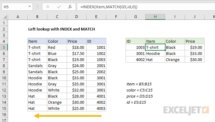
One of the key advantages of INDEX and MATCH over the VLOOKUP function is the ability to perform a «left lookup». Simply put, this just means a lookup where the ID column is to the right of the values you want to retrieve, as seen in the example below:

Case-sensitive lookup

By itself, the MATCH function is not case-sensitive. However, you use the EXACT function with INDEX and MATCH to perform a lookup that respects upper and lower case, as shown below:

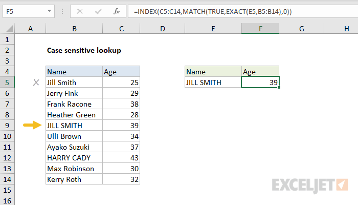
Note: this is an array formula and must be entered with control + shift + enter, except in Excel 365.

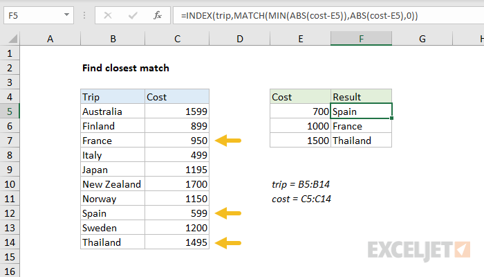
Closest match

Another example that shows off the flexibility of INDEX and MATCH is the problem of finding the closest match. In the example below, we use the MIN function together with the ABS function to create a lookup value and a lookup array inside the MATCH function. Essentially, we use MATCH to find the smallest difference. Then we use INDEX to retrieve the associated trip from column B.

Note: this is an array formula and must be entered with control + shift + enter, except in Excel 365.

Multiple criteria lookup

One of the trickiest problems in Excel is a lookup based on multiple criteria. In other words, a lookup that matches on more than one column at the same time. In the example below, we are using INDEX and MATCH and boolean logic to match on 3 columns: Item, Color, and Size:

Note: this is an array formula and must be entered with control + shift + enter, except in Excel 365.

More examples of INDEX + MATCH

Here are some more basic examples of INDEX and MATCH in action, each with a detailed explanation:

Источник

INDEX and MATCH with multiple criteria

Summary

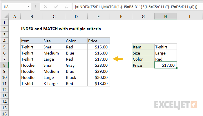
To lookup values with INDEX and MATCH, using multiple criteria, you can use an array formula. In the example shown, the formula in H8 is:

The result is $17.00, the Price of a Large Red T-shirt. This is an array formula and must be entered with with Control + Shift + Enter in Legacy Excel.

Note: In the current version of Excel, you can use the same approach with the XLOOKUP function.

Generic formula

Explanation

This is a more advanced formula. For basics, see How to use INDEX and MATCH.

Normally, an INDEX MATCH formula is configured with MATCH set to look through a one-column range and provide a match based on given criteria. Without concatenating values in a helper column, or in the formula itself, there’s no way to supply more than one criteria.

This formula works around this limitation by using boolean logic to create an array of ones and zeros to represent rows matching all 3 criteria, then using MATCH to match the first 1 found. The temporary array of ones and zeros is generated with this snippet:

Here we compare the item in H5 against all items, the size in H6 against all sizes, and the color in H7 against all colors. The initial result is three arrays of TRUE/FALSE results like this:

Tip: use F9 to see these results. Just select an expression in the formula bar, and press F9.

The math operation (multiplication) transforms the TRUE FALSE values to 1s and 0s:

After multiplication, we have a single array like this:

which is fed into the MATCH function as the lookup array, with a lookup value of 1:

At this point, the formula is a standard INDEX MATCH formula. The MATCH function returns 3 to INDEX:

and INDEX returns a final result of $17.00.

Array visualization

The arrays explained above can be difficult to visualize. The image below shows the basic idea. Columns B, C, and D correspond to the data in the example. Column F is created by the multiplying the three columns together. It is the array handed off to MATCH.

Non-array version

It is possible to add another INDEX to this formula, avoiding the need to enter as an array formula with control + shift + enter:

The INDEX function can handle arrays natively, so the second INDEX is added only to «catch» the array created with the boolean logic operation and return the same array again to MATCH. To do this, INDEX is configured with zero rows and one column. The zero row trick causes INDEX to return column 1 from the array (which is already one column anyway).

Why would you want the non-array version? Sometimes, people forget to enter an array formula with control + shift + enter, and the formula returns an incorrect result. So, a non-array formula is more «bulletproof». However, the tradeoff is a more complex formula.

Note: In Excel 365, it is not necessary to enter array formulas in a special way.

Источник

MATCH

Tip: Try using the new XMATCH function, an improved version of MATCH that works in any direction and returns exact matches by default, making it easier and more convenient to use than its predecessor.

The MATCH function searches for a specified item in a range of cells, and then returns the relative position of that item in the range. For example, if the range A1:A3 contains the values 5, 25, and 38, then the formula =MATCH(25,A1:A3,0) returns the number 2, because 25 is the second item in the range.

Tip: Use MATCH instead of one of the LOOKUP functions when you need the position of an item in a range instead of the item itself. For example, you might use the MATCH function to provide a value for the row_num argument of the INDEX function.

Syntax

MATCH(lookup_value, lookup_array, [match_type])

The MATCH function syntax has the following arguments:

lookup_value Required. The value that you want to match in lookup_array. For example, when you look up someone’s number in a telephone book, you are using the person’s name as the lookup value, but the telephone number is the value you want.

The lookup_value argument can be a value (number, text, or logical value) or a cell reference to a number, text, or logical value.

lookup_array Required. The range of cells being searched.

match_type Optional. The number -1, 0, or 1. The match_type argument specifies how Excel matches lookup_value with values in lookup_array. The default value for this argument is 1.

The following table describes how the function finds values based on the setting of the match_type argument.

MATCH finds the largest value that is less than or equal to lookup_value. The values in the lookup_array argument must be placed in ascending order, for example: . -2, -1, 0, 1, 2, . A-Z, FALSE, TRUE.

MATCH finds the first value that is exactly equal to lookup_value. The values in the lookup_array argument can be in any order.

MATCH finds the smallest value that is greater than or equal to lookup_value. The values in the lookup_array argument must be placed in descending order, for example: TRUE, FALSE, Z-A, . 2, 1, 0, -1, -2, . and so on.

MATCH returns the position of the matched value within lookup_array, not the value itself. For example, MATCH(«b», <«a»,»b»,»c «>,0) returns 2, which is the relative position of «b» within the array <«a»,»b»,»c»>.

MATCH does not distinguish between uppercase and lowercase letters when matching text values.

If MATCH is unsuccessful in finding a match, it returns the #N/A error value.

If match_type is 0 and lookup_value is a text string, you can use the wildcard characters — the question mark ( ?) and asterisk ( *) — in the lookup_value argument. A question mark matches any single character; an asterisk matches any sequence of characters. If you want to find an actual question mark or asterisk, type a tilde (

) before the character.

Example

Copy the example data in the following table, and paste it in cell A1 of a new Excel worksheet. For formulas to show results, select them, press F2, and then press Enter. If you need to, you can adjust the column widths to see all the data.

Источник

Updated 12/16/2022: Stay up to date on the latest from Excel and download Excel templates today.

If you want to look up a value in a table using one criterion, it’s simple. You can use a plain VLOOKUP formula. But if you want to use more than one criterion, what can you do? There are lots of ways to use several Microsoft Excel functions such as VLOOKUP, LOOKUP, MATCH, and INDEX. In this blog post, I’ll show you a few of those ways.

Get a better picture of your data.

Using two criteria to return a value from a table

Let’s look at a scenario where you want to use two criteria to return a value. Here’s the data you have:

The criteria are “Name” and “Product,” and you want them to return a “Qty” value in cell C18. Because the value that you want to return is a number, you can use a simple SUMPRODUCT() formula to look for the Name “James Atkinson” and the Product “Milk Pack” to return the Qty. The SUMPRODUCT formula in cell C18 looks like this:

=SUMPRODUCT((B3:B13=C16)*(C3:C13=C17)*(D3:D13))

What it does is look in the range B3:B13 for the value in cell C16, and in the range C3:C13 for the value in cell C17. When it finds both, it returns the value in column D, from the same row where it met both criteria. Here’s how it will look:

It returns the value 1, which corresponds to the value in cell D4 (“James Atkinson” in row 4 and also “Milk Pack” in the same row), thus returning the value in column D from that row. Let’s change the value in cell C5 from “Wine Bottle” to “Milk Pack” to see what happens with the formula in cell C18:

Because our formula found two lines where both criteria were met, it sums the values in column D in both rows, giving us a Qty of 6.

This technique cannot be used if you want to look for two criteria and return a text result. For instance, this, would not work:

You would be looking for the Name “James Atkinson” where the Qty is 1, and you’d like to return the Product name that matches these two criteria. This formula would give us a #VALUE error! Instead, you could use a formula using a combination of SUMPRODUCT, INDEX, and ROW functions, such as this one:

=INDEX(C3:C13,SUMPRODUCT((B3:B13=C16)*(D3:D13=C18)*ROW(C3:C13)),0)

You use the SUMPRODUCT function to find out the row where both criteria are met, and return the corresponding row number using the ROW function. Then you use SUMPRODUCT in the INDEX function to return the value in the array C3:C13 that is in the row number provided. The result will be like this:

Using Lookup and multivalued fields in queries

Learn more

You could also do this using a different technique, such as this formula in cell C17:

=LOOKUP(2,1/(B3:B13=C16)/(D3:D13=C18),(C3:C13))

The result will be the same as in the previous solution. What this formula does, is divide 1 by an array of True/False values (B3:B13=C16), and then by another array of True/False values (D3:D13=C18). This will return either 1 or a #DIV/0! error. If you use 2 as the lookup value, then the formula will match it with the last numeric value in the range, that is, the last row where both conditions are True. This is the “vector form” of the LOOKUP, so you can use it to get the corresponding value returned from C3:C13. I used 2 as the LOOKUP value, but it can be any number, starting at 1. If the formulas don’t find any match, you will, of course, get a #N/A error!

You could also use an array formula, using the MATCH function, like this:

{=INDEX(C3:C13,MATCH(1,(B3:B13=C16)*(D3:D13=C18),0))}

With this technique, you can use the MATCH function to find the row where both conditions are met. This returns a value of 1, which is matched to the 1 that is used as the lookup value of the MATCH function, thus returning us to the row where the conditions are met. Using the INDEX value, you can look for the value that is in the range C3:C13, which is in the row that was returned from the MATCH function. In this case, it was row 2, which corresponds to the second row in the range C3:C13.

Task management in Microsoft 365

Collaborate on shared Office documents, including Excel, Word, and PowerPoint.

Using multiple criteria to return a value from a table

All of these examples show you how to use two criteria for lookups. It’s also easy to use these formulas if you have more than two criteria-you just add them to the formulas. Here is how the formulas would look if you add one more criterion:

=SUMPRODUCT((B3:B13=C16)*(C3:C13=C17)*(E3:E13=C18)*(D3:D13))

=INDEX(C3:C13,SUMPRODUCT((B3:B13=C16)*(D3:D13=C18)*(E3:E13=C18)*ROW(C3:C13)),0)

=LOOKUP(2,1/(B3:B13=C16)/(D3:D13=C18)/(E3:E13=C18),(C3:C13))

{=INDEX(C3:C13,MATCH(1,(B3:B13=C16)*(D3:D13=C18)*(E3:E13=C18),0))}

Learn more

As you can see, depending on what’s in your data tables, you can use several different techniques using different Excel functions to look up values. Enjoy applying these to your own Excel spreadsheets.

Источник

Author: Oscar Cronquist Article last updated on November 08, 2021

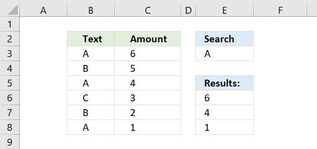
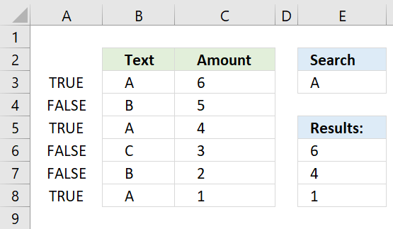
This article demonstrates how to use INDEX and MATCH functions to lookup and return multiple results. The lookup value is in cell E3, the lookup range is B3:B8.

Cells B3, B5, and B8 contains the lookup value, cell values in the corresponding cells in column C are returned. They are C3, C5, and C8.

There is actually a smaller formula that does the same thing: VLOOKUP — Return multiple values I also recommend the FILTER function if you are an Excel 365 user, the FILTER function is really easy to use.

The array formula in cell E6 extracts values from column C when the corresponding value in column B matches the value in cell E3.

The matching rows are 3, 5 and 8 so the array formula returns 3 values in cell range E6:E8.

=INDEX($C$3:$C$8, SMALL(IF(ISNUMBER(MATCH($B$3:$B$8, $E$3, 0)), MATCH(ROW($B$3:$B$8), ROW($B$3:$B$8)), «»), ROWS($A$1:A1)))

The formula above is an array formula, make sure you follow the instructions below on how to enter an array formula to make it work.

1. How to enter an array formula

To enter an array formula, type the formula in a cell then press and hold CTRL + SHIFT simultaneously, now press Enter once. Release all keys.

The formula bar now shows the formula enclosed with curly brackets telling you that you entered the formula successfully. Don’t enter the curly brackets yourself.

Now copy cell E6 and paste to cells below as far as needed.

2. Explaining formula in cell E6

Step 1 — Find matching values

The MATCH function matches a cell range against a single value returning an array.

MATCH($B$3:$B$8, $E$3, 0)

becomes

MATCH({«A»; «B»; «A»; «C»; «B»; «A»}, «A», 0)

and returns

{1; #N/A; 1; #N/A; #N/A; 1}.

If a value is equal to the search value MATCH function returns 1. If it is not equal the MATCH function returns #N/A.

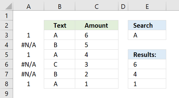
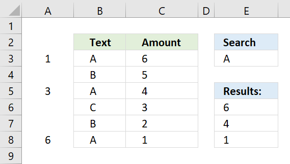
The picture above displays the array in column A.

Step 2 — Convert array values to boolean values

The IF function cant process error values so to solve that I am going to use the ISNUMBER function to convert the array values to boolean values.

ISNUMBER(MATCH($B$3:$B$8, $E$3, 0))

becomes

ISNUMBER({1; #N/A; 1; #N/A; #N/A; 1})

and returns

{TRUE; FALSE; TRUE; FALSE; FALSE; TRUE}.

The array is shown in column A, see picture below.

Step 3 — Identify rows

The IF function converts the boolean values into row numbers and blanks.

IF(ISNUMBER(MATCH($B$3:$B$8, $E$3, 0)), MATCH(ROW($B$3:$B$8), ROW($B$3:$B$8)), «»)

becomes

IF({TRUE; FALSE; TRUE; FALSE; FALSE; TRUE}, MATCH(ROW($B$3:$B$8), ROW($B$3:$B$8)), «»)

The MATCH and ROW functions calculate an array with sequential numbers, 1 to n, determined by the size of the cell range. In this case, $B$3:$B$8 has 6 values so the array becomes 1 to 6.

IF({TRUE; FALSE; TRUE; FALSE; FALSE; TRUE}, {1; 2; 3 ;4; 5; 6}, «»)

and returns

{1;»»;3;»»;»»;6}.

The picture below shows the relative row numbers for cell range B3:B8.

Step 4 — Get the k-th smallest row number

To be able to return the correct value the formula must know which value to get. The SMALL function determines the value to get based on row number.

SMALL(IF(ISNUMBER(MATCH($B$3:$B$8, $E$3, 0)), MATCH(ROW($B$3:$B$8), ROW($B$3:$B$8)), «»), ROWS($A$1:A1))

becomes

SMALL({1;»»;3;»»;»»;6}, ROWS($A$1:A1))

The ROWS function returns a number that changes when you copy the cell and paste to cells below.

SMALL({1;»»;3;»»;»»;6}, 1)

and returns 1.

In the next cell below ROWS($A$1:A1) changes to ROWS($A$1:A2) and returns 2.

Step 5 — Get values from column C using row numbers

The INDEX function returns a value from a given cell range based on a row and column number.

INDEX($C$3:$C$8, SMALL(IF(ISNUMBER(MATCH($B$3:$B$8, $E$3, 0)), MATCH(ROW($B$3:$B$8), ROW($B$3:$B$8)), «»), ROWS($A$1:A1)))

becomes

INDEX($C$3:$C$8, 1)

The first cell value in cell range $C$3:$C$8 is 6, the INDEX function returns 6 in cell E6.

3. Get Excel file

Array visualization

Non-array version

It is possible to add another INDEX to this formula, avoiding the need to enter as an array formula with control + shift + enter:

=INDEX(rng1,MATCH(1,INDEX((A1=rng2)*(B1=rng3)*(C1=rng4),0,1),0))

Note: In Excel 365, it is not necessary to enter array formulas in a special way.

Источник

What you’re trying to do is a cross tabulation (aka crosstab). The tool for doing that in Excel is called a PivotTable.

Unfortunately, pivot tables aren’t compatible with qualitative data, so to get this to work, you’re going to need to add a column, which represents your fed/not-fed data as a numeric value.

For instance, if you use =IF(B2="Not Fed",1,0) you will get a column in which if any animal is «Not Fed», you will get a one. (Note, you haven’t specified what you want to happen if the Fed? field is empty for a row, or has other surprizing value. You haven’t said what you want to happen in the case that "birds" -> {"not fed", "partially fed", "fed"}. What precise IF statement you use depends on your answers to these questions.)

Then you select the whole range with all three columns (or put the new column between these two, and select just the animals and your calculated column, and select «PivotTable report» from the Data menu.

The wizard will step you through a series of dialogs. On the first one, your data is in «Microsoft Excel list or database». On the second, if you selected your data before you started the wizard, it should default to your data range correctly.

On the third dialog, don’t hit Finish immediately. You have a bunch of options you need to set. First, on that dialog, you will be given a choice of where to put the new pivot table. I recommend putting your pivot table on a new sheet. Next, click «Layout…». Drag the «Animals» box into the left column («Row»). Drag the title to your new column into the
«Data» area in the middle; when you do that, it will show up as «Sum of nameoffield». Double click it, change the name to something like «Are any animals unfed?» and change the summary type to «Max», and click «Okay», then click «Okay» again to finish with the Layout dialog. You’re still on step 3 of the wizard dialog. Click «Options…». Unclick «Grand Total for Columns» and make sure «Grand Total for Rows» is on. Turn on «For Error Values Show» (very important for this) and set it to 0, and hit «Okay». Then, finally, you can hit «Finish» the wizard.

You should wind up with a new sheet that says:

Are any animals unfed?  
Animals Total
Cat     0
Dog     1

Now, you can enter into the column right after that, =IF(B3=1, "Some Animals Not Fed", "All Animals Fed") and so on down the column, and if any one animal in a type is «Not Fed», it will read «Some Animals Not Fed», otherwise «All Animals Fed»). You can now hide the B column, and see only:

Are any animals unfed?  
Animals 
Cat     All Animals Fed
Dog     Some Animals Not Fed

Источник

How to use INDEX and MATCH

Summary

The INDEX Function

The MATCH function

INDEX and MATCH together

Two-way lookup with INDEX and MATCH

Left lookup

Case-sensitive lookup

Closest match

Multiple criteria lookup

More examples of INDEX + MATCH

INDEX and MATCH with multiple criteria

Summary

Generic formula

Explanation

Array visualization

Non-array version

MATCH

Syntax

Example

Using two criteria to return a value from a table

Task management in Microsoft 365

Using multiple criteria to return a value from a table

Learn more

1. How to enter an array formula

2. Explaining formula in cell E6

Step 1 — Find matching values

Step 2 — Convert array values to boolean values

Step 3 — Identify rows

Step 4 — Get the k-th smallest row number

Step 5 — Get values from column C using row numbers

3. Get Excel file

Related post

Array visualization

Non-array version