
MATCH function
Tip: Try using the new XMATCH function, an improved version of MATCH that works in any direction and returns exact matches by default, making it easier and more convenient to use than its predecessor.
The MATCH function searches for a specified item in a range of cells, and then returns the relative position of that item in the range. For example, if the range A1:A3 contains the values 5, 25, and 38, then the formula =MATCH(25,A1:A3,0) returns the number 2, because 25 is the second item in the range.

Tip: Use MATCH instead of one of the LOOKUP functions when you need the position of an item in a range instead of the item itself. For example, you might use the MATCH function to provide a value for the row_num argument of the INDEX function.
Syntax
MATCH(lookup_value, lookup_array, [match_type])
The MATCH function syntax has the following arguments:
-
lookup_value Required. The value that you want to match in lookup_array. For example, when you look up someone’s number in a telephone book, you are using the person’s name as the lookup value, but the telephone number is the value you want.
The lookup_value argument can be a value (number, text, or logical value) or a cell reference to a number, text, or logical value.
-
lookup_array Required. The range of cells being searched.
-
match_type Optional. The number -1, 0, or 1. The match_type argument specifies how Excel matches lookup_value with values in lookup_array. The default value for this argument is 1.
The following table describes how the function finds values based on the setting of the match_type argument.
|
Match_type |
Behavior |
|
1 or omitted |
MATCH finds the largest value that is less than or equal to lookup_value. The values in the lookup_array argument must be placed in ascending order, for example: …-2, -1, 0, 1, 2, …, A-Z, FALSE, TRUE. |
|
0 |
MATCH finds the first value that is exactly equal to lookup_value. The values in the lookup_array argument can be in any order. |
|
-1 |
MATCH finds the smallest value that is greater than or equal tolookup_value. The values in the lookup_array argument must be placed in descending order, for example: TRUE, FALSE, Z-A, …2, 1, 0, -1, -2, …, and so on. |
-
MATCH returns the position of the matched value within lookup_array, not the value itself. For example, MATCH(«b»,{«a»,»b»,»c«},0) returns 2, which is the relative position of «b» within the array {«a»,»b»,»c»}.
-
MATCH does not distinguish between uppercase and lowercase letters when matching text values.
-
If MATCH is unsuccessful in finding a match, it returns the #N/A error value.
-
If match_type is 0 and lookup_value is a text string, you can use the wildcard characters — the question mark (?) and asterisk (*) — in the lookup_value argument. A question mark matches any single character; an asterisk matches any sequence of characters. If you want to find an actual question mark or asterisk, type a tilde (~) before the character.
Example
Copy the example data in the following table, and paste it in cell A1 of a new Excel worksheet. For formulas to show results, select them, press F2, and then press Enter. If you need to, you can adjust the column widths to see all the data.
|
Product |
Count |
|
|
Bananas |
25 |
|
|
Oranges |
38 |
|
|
Apples |
40 |
|
|
Pears |
41 |
|
|
Formula |
Description |
Result |
|
=MATCH(39,B2:B5,1) |
Because there is not an exact match, the position of the next lowest value (38) in the range B2:B5 is returned. |
2 |
|
=MATCH(41,B2:B5,0) |
The position of the value 41 in the range B2:B5. |
4 |
|
=MATCH(40,B2:B5,-1) |
Returns an error because the values in the range B2:B5 are not in descending order. |
#N/A |
Need more help?
You can quickly compare two lists in Excel for matches using the MATCH function, IF function, or highlighting row difference.
Manually searching for the difference between two lists can both be time-consuming and prone to errors. You will end up wasting a lot of time!
There are various inbuilt functions and features in Excel that can do this task of Excel compare two lists easily. Let’s look for various options that you can follow:
- Highlight Row Difference
- Compare Row using IF function
- Compare List using Match Function
Let’s look at each method one-by-one!
Don’t forget to download this Excel Workbook to follow along and compare two lists in Excel for matches:
Highlight Row Difference
You can easily highlight differences in value in each row using the conditional formatting feature in Excel. It will provide you with an idea of how many lines in the columns differ in values.
In the data below, you have two lists in Column A and Column B respectively.
Follow the steps below to highlight row difference:
STEP 1: Select both the columns.

STEP 2: Go to Home > Find & Select > Go To Special or simply press keys Ctrl + G and Select Special to open the Go To Special dialog box.

STEP 3: Select Row Difference and Click OK.

And, Voila!

All the values in Stock List 2 that do not match with the corresponding value in Stock List 1 have been highlighted.
STEP 4: You can mark these cells with color as well. Go to Home > Font Color > Select Red.


This will permanently highlight the cells in red font color for future reference.
Compare Row using IF function
You can use the IF Function to compare two lists in Excel for matches in the same row. If Function will return the value TRUE if the values match and FALSE if they don’t.
You can even add custom text to display the word “Match” when a criterion is met and “Not a Match” when it’s not met.
Let’s see how we can compare two lists in Excel for matches using IF Function:
STEP 1: We need to enter the IF function in a blank cell.
=IF(

STEP 2: Enter the first argument for the IF function – Logical_Test
What is your condition?
The value in cell D12 is equal to the value in cell C12.
=IF(D12=C12,

STEP 3: Enter the second argument for the IF function – Value_if_true
What value should be displayed if the condition is true?
The text displayed should be Match if D12 is equal to C12.
=IF(D12=C12,“Match”,

STEP 4: Enter the third argument for the IF function – Value_if_false
What value should be displayed if the condition is false?
The text displayed should be Not a Match if D12 is not equal to C12.
=IF(D12=C12,”Match”,“Not a Match”)

STEP 5: Apply the same formula to the rest of the cells by dragging the lower right corner downwards.

Compare List using Match Function
Before we understand how to compare two lists in Excel for matches, let’s first go through the basics of what the MATCH function Excel does.
What does it do?
It returns the position of an item in a range.
Formula breakdown:
=MATCH(lookup_value, lookup_array, [match_type])
What it means:
=MATCH(lookup this value, from this list or range of cells, return me the Exact Match).
I am sure that you have come across many occasions where you have two lists of data and want to know if a specific item in List1 exists in List2.
Well, I have!
With the MATCH function, you can verify if a cell´s item in List1 exists in List2.
The function will return the row position of that item in List2 hence confirming that it exists. If you get a #N/A it means that the cell´s item does not exist in List2.
You can then go ahead and filter your List1 with either the values returned or the #N/As.
Here are our 2 Lists:


STEP 1: We need to enter the MATCH function in a blank cell:
=MATCH(

STEP 2: Enter the first argument for the MATCH function – Lookup_value
What is the value you want to check?
Select the cell containing the List1 value, as this is what we want to check against List2.
=MATCH(C12,

STEP 3: Enter the second argument for the MATCH function – Lookup_array
What is the list you want to check against?
Select the entire List2.

And ensure to press F4 to make it an absolute reference.
=MATCH(C12, list2!$C$12:$C:21,

STEP 4: Enter the third argument for the MATCH function – Match_type
How specific is your matching? We want an exact match so place in 0.
=MATCH(C12, list2!$C$12:$C:21, 0)

STEP 5: Apply the same formula to the rest of the cells by dragging the lower right corner downwards.

You now have all of the results!
You can see which row numbers the items exist in List2. For example, Mon45657 in List1 exists in List2 Row 9! If it does not exist in List2, then #N/A is displayed.

Using either of the three ways mentioned in this article, you can easily compare two lists in Excel for matches!
How to Compare Two Lists in Excel? (Top 6 Methods)
Below are the six different methods used to compare two lists of a column in Excel for matches and differences.
- Method 1: Compare Two Lists Using Equal Sign Operator
- Method 2: Match Data by Using the Row Difference Technique
- Method 3: Match Row Difference by Using the IF Condition
- Method 4: Match Data Even If There is a Row Difference
- Method 5: Highlight All the Matching Data using Conditional Formatting
- Method 6: Partial Matching Technique
Table of contents
- How to Compare Two Lists in Excel? (Top 6 Methods)
- #1 Compare Two Lists Using Equal Sign Operator
- #2 Match Data by Using Row Difference Technique
- #3 Match Row Difference by Using IF Condition
- #4 Match Data Even If There is a Row Difference
- #5 Highlight All the Matching Data
- #6 Partial Matching Technique
- Things to Remember
- Recommended Articles
Now, let us discuss each of the methods in detail with an example: –
You can download this Compare Two Lists Excel Template here – Compare Two Lists Excel Template
#1 Compare Two Lists Using Equal Sign Operator
We must follow the below steps to compare the two lists.
- Immediately after the two columns, we must insert a new column called “Status” in the next column.

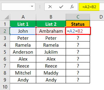
- Now, we must put the formula in cell C2 as =A2=B2.

- This formula tests whether the cell A2 value is equal to cell B2. If both cell values are matched, we will get TRUE or FALSE results.

- We will drag the formula to cell C9 to determine the other values.


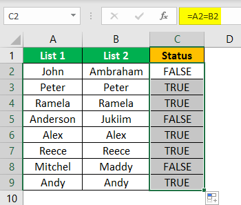
Wherever we have the same values in common rows, we get the result as “TRUE” or “FALSE.”
#2 Match Data by Using Row Difference Technique
You might not have used the “Row Difference” technique at your workplace. But today, we will show you how to use this technique to match data row by row.
- Step 1: To highlight non-matching cells row by row, we must select the entire data first.

- Step 2: Now, we must press the excel shortcut keyAn Excel shortcut is a technique of performing a manual task in a quicker way.read more “F5” to open the “Go to Special” tool.
![]()
- Step 3: Press the “F5” key to open this window. In the “Go To” window, press the “Special” tab.

- Step 4: In the next window, we must go to the “Go To Special” and choose the “Row differences” option. Then, click on “OK.”

We will get the following result.

As shown in the above window, it has selected the cells wherever there is a row difference. Therefore, we must fill in some colors to highlight the row difference values.

#3 Match Row Difference by Using IF Condition
How can we leave out the IF condition when we want to match data row by row? In the first example, we have either “TRUE” or “FALSE.” But what if we need a different result instead of the default results of either “TRUE or FALSE.” Assume we need a result as “Matching” if there is no row difference, and the result should be “Not Matching” if there is a row difference.
- Step 1: First, we must open the IF condition in cell C2.

- Step 2: Then, apply the logical testA logical test in Excel results in an analytical output, either true or false. The equals to operator, “=,” is the most commonly used logical test.read more as A2=B2.
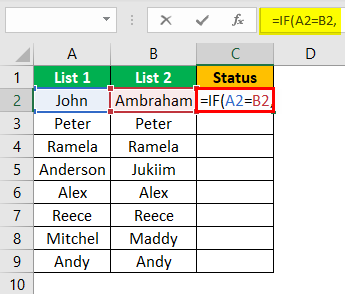
- Step 3: We must enter the result criteria if the logical test is “TRUE.” In this scenario, the result criteria are “Matching,” If the row does not match, we need the result as “Not Matching.”

- Step 4: Next, we need to apply the formula to get the result.
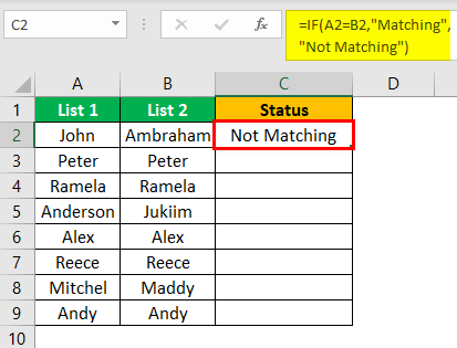
- Step 5: We must drag the formula to cell C9 to determine the other values.

#4 Match Data Even If There is a Row Difference
The matching data on the row differences method may not always work; the value may be in other cells too. So we need to use different technologies in these scenarios.
Now, look at the below data.

In the above image, we have two lists of numbers. We need to compare list 2 wish list 1. So let us use our favorite function VLOOKUPThe VLOOKUP excel function searches for a particular value and returns a corresponding match based on a unique identifier. A unique identifier is uniquely associated with all the records of the database. For instance, employee ID, student roll number, customer contact number, seller email address, etc., are unique identifiers.
read more.

So, if the data matches, we get the number; otherwise, we get the error value as #N/A.
Showing error values does not look good. So instead of showing the error, let us replace them with the word “Not Available.” For this, use the IFERROR function in ExcelThe IFERROR function in Excel checks a formula (or a cell) for errors and returns a specified value in place of the error.read more.

#5 Highlight All the Matching Data
If you are not a fan of Excel formulasThe term «basic excel formula» refers to the general functions used in Microsoft Excel to do simple calculations such as addition, average, and comparison. SUM, COUNT, COUNTA, COUNTBLANK, AVERAGE, MIN Excel, MAX Excel, LEN Excel, TRIM Excel, IF Excel are the top ten excel formulas and functions.read more, do not worry. We can still match data without the formula. For example, using simple conditional formatting in ExcelConditional formatting is a technique in Excel that allows us to format cells in a worksheet based on certain conditions. It can be found in the styles section of the Home tab.read more, we can highlight all the matching data of two lists.
- Step 1: We must first select the data.

- Step 2: Now, we must go to “Conditional Formatting” and choose “Highlight Cell Rules” >> “Duplicate Values.”

- Step 3: As a result, we can see the “Duplicate Cell Values” formatting window.

- Step 4: We can choose the different formatting colors from the drop-down list in ExcelA drop-down list in excel is a pre-defined list of inputs that allows users to select an option.read more. Select the first formatting color and press the “OK” button.

- Step 5: This will highlight all the matching data from the two lists.

- Step 6: Just in case, instead of highlighting all the matching data, if we want to highlight not matching data, then we can go to the “Duplicate Values” window and choose the option “Unique.”

As a result, it will highlight all the non-matching values, as shown below.

#6 Partial Matching Technique
We have seen the issue of not having full or the same data in two lists. For example, if the List 1 data has “ABC Pvt Ltd.“ In List 2, we have “ABC” only. In these cases, all our default formulas and tools are not recognized. Therefore, we need to employ the special character asterisk (*) to match partial values in these cases.

In List 1, we have the company name and revenue details. In List 2, we have company names but not exact values as in List 1. It is a tricky situation that we all have faced at our workplace.
In such cases, still, we can match data by using a special character asterisk (*).

We get the following result.

We will drag the formula to cell E9 to determine the other values.

The wildcard character asterisk (*) was used to represent any number of characters so that it will match the full character for the word “ABC” as “ABC Pvt Ltd.”
Things to Remember
- The use of the above techniques for comparing two lists in Excel upon the data structure.
- If the data is not organized, row-by-row matching is not the best suited.
- VLOOKUP is the often-used formula to match values.
Recommended Articles
This article is a guide to Compare Two Lists in Excel. We discuss the top 6 methods to compare two columns list in Excel for the match, along with examples and a downloadable Excel template. You may learn more about Excel from the following articles: –
- Compare Two Excel Columns Using Vlookup
- Partial Match with Vlookup
- Compare Two Excel Columns
- Shade Alternate Rows in Excel
![]()
Download Article
![]()
Download Article
One of Microsoft Excel’s many capabilities is the ability to compare two lists of data, identifying matches between the lists and identifying which items are found in only one list. This is useful when comparing financial records or checking to see if a particular name is in a database. You can use the MATCH function to identify and mark matching or non-matching records, or you can use conditioning formatting with the COUNTIF function. The following steps tell you how to use each to match your data.
-

1
Copy the data lists onto a single worksheet. Excel can work with multiple worksheets within a single workbook, or with multiple workbooks, but you’ll find comparing the lists easier if you copy their information onto a single worksheet.
-
2
Give each list item a unique identifier. If your two lists don’t share a common way to identify them, you may need to add an additional column to each data list that identifies that item to Excel so that it can see if an item in a given list is related to an item in the other list. The nature of this identifier will depend on the kind of data you are trying to match. You will need an identifier for each column list.
- For financial data associated with a given period, such as with tax records, this could be the description of an asset, the date the asset was acquired, or both. In some cases, an entry may be identified with a code number; however, if the same system is not used for both lists, this identifier may create matches where there are none or ignore matches that should be made.
- In some cases, you can take items from one list and combine them with items from another list to create an identifier, such as a physical asset description and the year it was purchased. To create such an identifier, you concatenate (add, combine) data from two or more cells using the ampersand (&). To combine an item description in cell F3 with a date in cell G3, separated by a space, you’d enter the formula ‘=F3&» «&G3’ in another cell in that row, such as E3. If you wanted to include only the year in the identifier (because one list uses full dates and the other uses only years), you’d include the YEAR function by entering ‘=F3&» «&YEAR(G3)’ in cell E3 instead. (Do not include the single quotes; they are there only to indicate the example.)
- Once you’ve created the formula, you can copy it into all other cells of the identifier column by selecting the cell with the formula and dragging the fill handle over the other cells of the column where you want to copy the formula. When you release your mouse button, each cell you dragged over will be populated with the formula, with the cell references adjusted to the appropriate cells in the same row.
Advertisement
-
3
Standardize data where possible. While the mind recognizes that «Inc.» and «Incorporated» mean the same thing, Excel doesn’t unless you have it re-format one word or the other. Likewise, you may consider values such as $11,950 and $11,999.95 as close enough to match, but Excel won’t unless you tell it to.
- You can deal with some abbreviations, such as «Co» for «Company» and «Inc» for «Incorporated by using LEFT string function to truncate the additional characters. Other abbreviations, such as «Assn» for «Association,» may best be dealt with by establishing a data entry style guide and then writing a program to look up and correct improper formats.
- For strings of numbers, such as ZIP codes where some entries include the ZIP+4 suffix and others don’t, you can again use the LEFT string function to recognize and match only the primary ZIP codes. To have Excel recognize numeric values that are close but not the same, you can use the ROUND function to round close values to the same number and match them.
- Extra spaces, such as typing two spaces between words instead of one, can be removed by using the TRIM function.
-
4
Create columns for the comparison formula. Just as you had to create columns for the list identifiers, you’ll need to create columns for the formula that does the comparing for you. You’ll need one column for each list.
- You’ll want to label these columns with something like «Missing?»
-
5
Enter the comparison formula in each cell. For the comparison formula, you’ll use the MATCH function nested inside another Excel function, ISNA.
- The formula takes the form of «=ISNA(MATCH(G3,$L$3:$L$14,FALSE))», where a cell of the identifier column of the first list is compared against each of the identifiers in the second list to see if it matches one of them. If it doesn’t match, a record is missing, and the word «TRUE» will be displayed in that cell. If it does match, the record is present, and the word «FALSE» will be displayed. (When entering the formula, do not include the enclosing quotes.)
- You can copy the formula into the remaining cells of the column the same way you copied the cell identifier formula. In this case, only the cell reference for the identifier cell changes, as putting the dollar signs in front of the row and column references for the first and last cells in the list of the second cell identifiers makes them absolute references.
- You can copy the comparison formula for the first list into the first cell of the column for the second list. You’ll then have to edit the cell references so that «G3» is replaced with the reference for the first identifier cell of the second list and «$L$3:$L$14» is replaced with the first and last identifier cell of the second list. (Leave the dollar signs and colon alone.) You can then copy this edited formula into the remaining cells in the comparison row of the second list.
-
6
Sort the lists to see non-matching values more easily, if necessary. If your lists are large, you may need to sort them to put all the non-matching values together. The instructions in the substeps below will convert the formulas to values to avoid recalculation errors, and if your lists are large, will avoid a long recalculation time.
- Drag your mouse over all the cells in a list to select it.
- Select Copy from the Edit menu in Excel 2003 or from the Clipboard group of the Home ribbon in Excel 2007 or 2010.
- Select Paste Special from the Edit menu in Excel 2003 or from the Paste dropdown button in the Clipboard group of Excel 2007 or 2010s Home ribbon.
- Select «Values» from the Paste As list in the Paste Special dialog box. Click OK to close the dialog.
- Select Sort from the Data menu in Excel 2003 or the Sort and Filter group of the Data ribbon in Excel 2007 or 2010.
- Select «Header row» from the «My data range has» list in the Sort By dialog, select «Missing?» (or the name you actually gave the comparison column header) and click OK.
- Repeat these steps for the other list.
-
7
Compare the non-matching items visually to see why they don’t match. As noted previously, Excel is designed to look for exact data matches unless you set it up to look for approximate ones. Your non-match could be as simple as an accidental transposing of letters or digits. It could also be something that requires independent verification, such as checking to see if listed assets needed to be reported in the first place.


Advertisement
-
1
Copy the data lists onto a single worksheet.
-
2
Decide in which list you want to highlight matching or non-matching records. If you want to highlight records in only one list, you’ll probably want to highlight the records unique to that list; that is, records that don’t match records in the other list. If you want to highlight records in both lists, you’ll want to highlight records that do match each other. For the purposes of this example, we’ll assume the first list takes up cells G3 through G14 and the second list takes up cells L3 through L14.
-
3
Select the items in the list you wish to highlight unique or matching items in. If you wish to highlight matching items in both lists, you’ll have to select the lists one at a time and apply the comparison formula (described in the next step) to each list.
-
4
Apply the appropriate comparison formula. To do this, you’ll have to access the Conditional Formatting dialog in your version of Excel. In Excel 2003, you do so by selecting Conditional Formatting from the Format menu, while in Excel 2007 and 2010, you click the Conditional Formatting button in the Styles group of the Home ribbon. Select the rule type as «Formula» and enter your formula in the Edit the Rule Description field.
- If you want to highlight records unique to the first list, the formula would be «=COUNTIF($L$3:$L$14,G3=0)», with the range of cells of the second list rendered as absolute values and the reference to the first cell of the first list as a relative value. (Don’t enter the close quotes.)
- If you want to highlight records unique to the second list, the formula would be «=COUNTIF($G$3:$G$14,L3=0)», with the range of cells of the first list rendered as absolute values and the reference to the first cell of the second list as a relative value. (Don’t enter the close quotes.)
- If you want to highlight the records in each list that are found in the other list, you’ll need two formulas, one for the first list and one for the second. The formula for the first list is «=COUNTIF($L$3:$L$14,G3>0)», while the formula for the second list is COUNTIF($G$3:$G$14,L3>0)». As noted previously, you select the first list to apply its formula and then select the second list to apply its formula.
- Apply whatever formatting you want to highlight the records being flagged. Click OK to close the dialog.


Advertisement
Ask a Question
200 characters left
Include your email address to get a message when this question is answered.
Submit
Advertisement
Video
-
Instead of using a cell reference with the COUNTIF conditional formatting method, you can enter a value to be searched for and flag one or more lists for instances of that value.
-
To simplify the comparison forms, you can create names for your list, such as «List1» and «List2.» Then, when writing the formulas, these list names can substitute for the absolute cell ranges used in the examples above.
Thanks for submitting a tip for review!
Advertisement
About This Article
Thanks to all authors for creating a page that has been read 107,172 times.
Is this article up to date?
This article explains in simple terms how to use INDEX and MATCH together to perform lookups. It takes a step-by-step approach, first explaining INDEX, then MATCH, then showing you how to combine the two functions together to create a dynamic two-way lookup. There are more advanced examples further down the page.
INDEX function | MATCH function | INDEX and MATCH | 2-way lookup | Left lookup | Case-sensitive | Closest match | Multiple criteria | More examples
The INDEX Function
The INDEX function in Excel is fantastically flexible and powerful, and you’ll find it in a huge number of Excel formulas, especially advanced formulas. But what does INDEX actually do? In a nutshell, INDEX retrieves the value at a given location in a range. For example, let’s say you have a table of planets in our solar system (see below), and you want to get the name of the 4th planet, Mars, with a formula. You can use INDEX like this:
=INDEX(B3:B11,4)

INDEX returns the value in the 4th row of the range.
Video: How to look things up with INDEX
What if you want to get the diameter of Mars with INDEX? In that case, we can supply both a row number and a column number, and provide a larger range. The INDEX formula below uses the full range of data in B3:D11, with a row number of 4 and column number of 2:
=INDEX(B3:D11,4,2)

INDEX retrieves the value at row 4, column 2.
To summarize, INDEX gets a value at a given location in a range of cells based on numeric position. When the range is one-dimensional, you only need to supply a row number. When the range is two-dimensional, you’ll need to supply both the row and column number.
At this point, you may be thinking «So what? How often do you actually know the position of something in a spreadsheet?»
Exactly right. We need a way to locate the position of things we’re looking for.
Enter the MATCH function.
The MATCH function
The MATCH function is designed for one purpose: find the position of an item in a range. For example, we can use MATCH to get the position of the word «peach» in this list of fruits like this:
=MATCH("peach",B3:B9,0)

MATCH returns 3, since «Peach» is the 3rd item. MATCH is not case-sensitive.
MATCH doesn’t care if a range is horizontal or vertical, as you can see below:
=MATCH("peach",C4:I4,0)

Same result with a horizontal range, MATCH returns 3.
Video: How to use MATCH for exact matches
Important: The last argument in the MATCH function is match_type. Match_type is important and controls whether matching is exact or approximate. In many cases you will want to use zero (0) to force exact match behavior. Match_type defaults to 1, which means approximate match, so it’s important to provide a value. See the MATCH page for more details.
INDEX and MATCH together
Now that we’ve covered the basics of INDEX and MATCH, how do we combine the two functions in a single formula? Consider the data below, a table showing a list of salespeople and monthly sales numbers for three months: January, February, and March.

Let’s say we want to write a formula that returns the sales number for February for a given salesperson. From the discussion above, we know we can give INDEX a row and column number to retrieve a value. For example, to return the February sales number for Frantz, we provide the range C3:E11 with a row 5 and column 2:
=INDEX(C3:E11,5,2) // returns $5194
But we obviously don’t want to hardcode numbers. Instead, we want a dynamic lookup.
How will we do that? The MATCH function of course. MATCH will work perfectly for finding the positions we need. Working one step at a time, let’s leave the column hardcoded as 2 and make the row number dynamic. Here’s the revised formula, with the MATCH function nested inside INDEX in place of 5:
=INDEX(C3:E11,MATCH("Frantz",B3:B11,0),2)
Taking things one step further, we’ll use the value from H2 in MATCH:
=INDEX(C3:E11,MATCH(H2,B3:B11,0),2)

MATCH finds «Frantz» and returns 5 to INDEX for row.
To summarize:
- INDEX needs numeric positions.
- MATCH finds those positions.
- MATCH is nested inside INDEX.
Let’s now tackle the column number.
Two-way lookup with INDEX and MATCH
Above, we used the MATCH function to find the row number dynamically, but hardcoded the column number. How can we make the formula fully dynamic, so we can return sales for any given salesperson in any given month? The trick is to use MATCH twice – once to get a row position, and once to get a column position.
From the examples above, we know MATCH works fine with both horizontal and vertical arrays. That means we can easily find the position of a given month with MATCH. For example, this formula returns the position of March, which is 3:
=MATCH("Mar",C2:E2,0) // returns 3
But of course we don’t want to hardcode any values, so let’s update the worksheet to allow the input of a month name, and use MATCH to find the column number we need. The screen below shows the result:

A fully dynamic, two-way lookup with INDEX and MATCH.
=INDEX(C3:E11,MATCH(H2,B3:B11,0),MATCH(H3,C2:E2,0))
The first MATCH formula returns 5 to INDEX as the row number, the second MATCH formula returns 3 to INDEX as the column number. Once MATCH runs, the formula simplifies to:
=INDEX(C3:E11,5,3)
and INDEX correctly returns $10,525, the sales number for Frantz in March.
Note: you could use Data Validation to create dropdown menus to select salesperson and month.
Video: How to do a two-way lookup with INDEX and MATCH
Video: How to debug a formula with F9 (to see MATCH return values)
Left lookup
One of the key advantages of INDEX and MATCH over the VLOOKUP function is the ability to perform a «left lookup». Simply put, this just means a lookup where the ID column is to the right of the values you want to retrieve, as seen in the example below:

Read a detailed explanation here.
Case-sensitive lookup
By itself, the MATCH function is not case-sensitive. However, you use the EXACT function with INDEX and MATCH to perform a lookup that respects upper and lower case, as shown below:

Read a detailed explanation here.
Note: this is an array formula and must be entered with control + shift + enter, except in Excel 365.
Closest match
Another example that shows off the flexibility of INDEX and MATCH is the problem of finding the closest match. In the example below, we use the MIN function together with the ABS function to create a lookup value and a lookup array inside the MATCH function. Essentially, we use MATCH to find the smallest difference. Then we use INDEX to retrieve the associated trip from column B.

Read a detailed explanation here.
Note: this is an array formula and must be entered with control + shift + enter, except in Excel 365.
Multiple criteria lookup
One of the trickiest problems in Excel is a lookup based on multiple criteria. In other words, a lookup that matches on more than one column at the same time. In the example below, we are using INDEX and MATCH and boolean logic to match on 3 columns: Item, Color, and Size:

Read a detailed explanation here. You can use this same approach with XLOOKUP.
Note: this is an array formula and must be entered with control + shift + enter, except in Excel 365.
More examples of INDEX + MATCH
Here are some more basic examples of INDEX and MATCH in action, each with a detailed explanation:
- Basic INDEX and MATCH exact (features Toy Story)
- Basic INDEX and MATCH approximate (grades)
- Two-way lookup with INDEX and MATCH (approximate match)