Match functions in excel - Word и Excel - помощь в работе с программами

MATCH function

Tip: Try using the new XMATCH function, an improved version of MATCH that works in any direction and returns exact matches by default, making it easier and more convenient to use than its predecessor.

The MATCH function searches for a specified item in a range of cells, and then returns the relative position of that item in the range. For example, if the range A1:A3 contains the values 5, 25, and 38, then the formula =MATCH(25,A1:A3,0) returns the number 2, because 25 is the second item in the range.

Tip: Use MATCH instead of one of the LOOKUP functions when you need the position of an item in a range instead of the item itself. For example, you might use the MATCH function to provide a value for the row_num argument of the INDEX function.

Syntax

MATCH(lookup_value, lookup_array, [match_type])

The MATCH function syntax has the following arguments:

lookup_value Required. The value that you want to match in lookup_array. For example, when you look up someone’s number in a telephone book, you are using the person’s name as the lookup value, but the telephone number is the value you want.

The lookup_value argument can be a value (number, text, or logical value) or a cell reference to a number, text, or logical value.
lookup_array Required. The range of cells being searched.
match_type Optional. The number -1, 0, or 1. The match_type argument specifies how Excel matches lookup_value with values in lookup_array. The default value for this argument is 1.

The following table describes how the function finds values based on the setting of the match_type argument.

Match_type	Behavior
1 or omitted	MATCH finds the largest value that is less than or equal to *lookup_value. The values in the lookup_array* argument must be placed in ascending order, for example: …-2, -1, 0, 1, 2, …, A-Z, FALSE, TRUE.
0	MATCH finds the first value that is exactly equal to *lookup_value. The values in the lookup_array* argument can be in any order.
-1	MATCH finds the smallest value that is greater than or equal tolookup_value. The values in the *lookup_array* argument must be placed in descending order, for example: TRUE, FALSE, Z-A, …2, 1, 0, -1, -2, …, and so on.

MATCH returns the position of the matched value within lookup_array, not the value itself. For example, MATCH(«b»,{«a»,»b»,»c«},0) returns 2, which is the relative position of «b» within the array {«a»,»b»,»c»}.
MATCH does not distinguish between uppercase and lowercase letters when matching text values.
If MATCH is unsuccessful in finding a match, it returns the #N/A error value.
If match_type is 0 and lookup_value is a text string, you can use the wildcard characters — the question mark (?) and asterisk (*) — in the lookup_value argument. A question mark matches any single character; an asterisk matches any sequence of characters. If you want to find an actual question mark or asterisk, type a tilde (~) before the character.

Example

Copy the example data in the following table, and paste it in cell A1 of a new Excel worksheet. For formulas to show results, select them, press F2, and then press Enter. If you need to, you can adjust the column widths to see all the data.

Product	Count
Bananas	25
Oranges	38
Apples	40
Pears	41
Formula	Description	Result
=MATCH(39,B2:B5,1)	Because there is not an exact match, the position of the next lowest value (38) in the range B2:B5 is returned.	2
=MATCH(41,B2:B5,0)	The position of the value 41 in the range B2:B5.	4
=MATCH(40,B2:B5,-1)	Returns an error because the values in the range B2:B5 are not in descending order.	#N/A

Need more help?

Want more options?

Explore subscription benefits, browse training courses, learn how to secure your device, and more.

Communities help you ask and answer questions, give feedback, and hear from experts with rich knowledge.

Источник

The MATCH function is used to determine the position of a value in a range or array. For example, in the screenshot above, the formula in cell E6 is configured to get the position of the value in cell D6. The MATCH function returns 5 because the lookup value («peach») is in the 5th position in the range B6:B14:

=MATCH(D6,B6:B14,0) // returns 5

The MATCH function can perform exact and approximate matches and supports wildcards (* ?) for partial matches. There are 3 separate match modes (set by the match_type argument), as described below.

Note: the MATCH function will always return the first match. If you need to return the last match (reverse search) see the XMATCH function. If you want to return all matches, see the FILTER function.

MATCH only supports one-dimensional arrays or ranges, either vertical or horizontal. However, you can use MATCH to locate values in a two-dimensional range or table by giving MATCH the single column (or row) that contains the lookup value. You can even use MATCH twice in a single formula to find a matching row and column at the same time.

Frequently, the MATCH function is combined with the INDEX function to retrieve a value at a certain (matched) position. In other words, MATCH figures out the position, and INDEX returns the value at that position. For a detailed overview with simple examples, see How to use INDEX and MATCH.

Match type information

Match type is optional. If not provided, match_type defaults to 1 (exact or next smallest). When match_type is 1 or -1, it is sometimes referred to as an «approximate match». However, keep in mind that MATCH will always perform an exact match when possible, as noted in the table below:

Match type	Behavior	Details
1	Approximate	MATCH finds the largest value less than or equal to the lookup value. The lookup array must be sorted in ascending order.
0	Exact	MATCH finds the first value equal to the lookup value. The lookup array does not need to be sorted.
-1	Approximate	MATCH finds the smallest value greater than or equal to the lookup value. The lookup array must be sorted in descending order.
(omitted)	Approximate	When match_type is omitted, it defaults to 1 with behavior as explained above.

Caution: Be sure to set match_type to zero (0) if you need an exact match. The default setting of 1 can cause MATCH to return results that look normal but are in fact incorrect. Explicitly providing a value for match_type, is a good reminder of what behavior is expected.

Exact match

When match_type is zero (0), MATCH performs an exact match only. In the example below, the formula in E3 is:

=MATCH(E2,B3:B11,0) // returns 4

In the formula above, the lookup value comes from cell E2. If the lookup value is hardcoded into the formula, it must be enclosed in double quotes («»), since it is a text value:

=MATCH("Mars",B3:B11,0)

Note: MATCH is not case-sensitive, so «Mars» and «mars» will both return 4.

Approximate match

When match_type is set to 1, MATCH will perform an approximate match on values sorted A-Z, finding the largest value less than or equal to the lookup value. In the example shown below, the formula in E3 is:

=MATCH(E2,B3:B11,1) // returns 5

Wildcard match

When match_type is set to zero (0), MATCH can use wildcards. In the example shown below, the formula in E3 is:

=MATCH(E2,B3:B11,0) // returns 6

This is equivalent to:

=MATCH("pq*",B3:B11,0)

INDEX and MATCH

The MATCH function is commonly used together with the INDEX function. The resulting formula is called «INDEX and MATCH». For example, in the screen below, INDEX and MATCH are used to return the cost of a code entered in cell F4. The formula in F5 is:

=INDEX(C5:C12,MATCH(F4,B5:B12,0)) // returns 150

In this example, MATCH is set up to perform an exact match. The MATCH function locates the code ABX-075 and returns its position (7) directly to the INDEX function as the row number. The INDEX function then returns the 7th value from the range C5:C12 as a final result. The formula is solved like this:

=INDEX(C5:C12,MATCH(F4,B5:B12,0))
=INDEX(C5:C12,7)
=150

See below for more examples of the MATCH function. For an overview of how to use INDEX and MATCH with many examples, see: How to use INDEX and MATCH.

Case-sensitive match

The MATCH function is not case-sensitive. However, MATCH can be configured to perform a case-sensitive match when combined with the EXACT function in a generic formula like this:

=MATCH(TRUE,EXACT(lookup_value,array),0))

The EXACT function compares every value in array with the lookup_value in a case-sensitive manner. This formula is explained with an INDEX and MATCH example here.

Notes

MATCH is not case-sensitive.
MATCH returns the #N/A error if no match is found.
MATCH only works with text up to 255 characters in length.
In case of duplicates, MATCH returns the first match.
If match_type is -1 or 1, the lookup_array must be sorted as noted above.
If match_type is 0, the lookup_value can contain the wildcards.
The MATCH function is frequently used together with the INDEX function.

Источник

На чтение 2 мин

Функция ПОИСКПОЗ в Excel используют для поиска точной позиции искомого значения в списке или массиве данных.

Содержание

Что возвращает функция
Синтаксис
Аргументы функции
Дополнительная информация
Примеры использования функции ПОИСКПОЗ в Excel

Что возвращает функция

Возвращает число, соответствующее позиции искомого значения.

Больше лайфхаков в нашем Telegram Подписаться

Синтаксис

=MATCH(lookup_value, lookup_array, [match_type]) — английская версия

=ПОИСКПОЗ(искомое_значение;просматриваемый_массив;[тип_сопоставления]) — русская версия

Аргументы функции

lookup_value (искомое_значение) — значение, с которым вы хотите сопоставить данные из массива или списка данных;
lookup_array (просматриваемый_массив) — диапазон ячеек в котором вы осуществляете поиск искомых данных;
[match_type] ([тип_сопоставления]) — (не обязательно) — этот аргумент определяет каким образом, будет осуществлен поиск. Допустимые значения для аргумента: «-1», «0», «1» (подробней читайте ниже).

Дополнительная информация

Чаще всего функция MATCH используется в сочетании с функцией INDEX (ИНДЕКС);
Подстановочные знаки могут использоваться в аргументах функции в тех случаях, когда значение поиска — текстовая строка;
При использовании функции ПОИСКПОЗ регистр букв не учитывается;
Функция возвращает #N/A ошибку, если искомое значение не найдено;
Аргумент match_type (тип_сопоставления) определяет каким образом, будет осуществлен поиск:
— Если аргумент match_type (тип_сопоставления) = 0, то это критерий точного соответствия. Он возвращает первую точную позицию соответствия (или ошибку, если совпадения нет);
— Если аргумент match_type (тип_сопоставления) = 1 (по умолчанию), то в таком случае данные должны быть отсортированы в порядке возрастания для этой опции. Функция возвращает наибольшее значение, равное или меньшее значения поиска.
— Если аргумент match_type (тип_сопоставления) = -1, то в таком случае данные должны быть отсортированы в порядке убывания для этой опции. Функция возвращает наименьшее и наибольшее значения поиска.

Примеры использования функции ПОИСКПОЗ в Excel

Источник

Improve Article

Save Article

Like Article

Read

Discuss

Improve Article

Save Article

Like Article

Excel contains many useful functions and such a function is the ‘MATCH()’ function. It is basically used to get the relative position of a specific item from a range of cells(i.e. from a row or a column or from a table). This function also supports exact and approximate match like VLOOKUP() function. Generally, MATCH() function is used with the INDEX() function.

With the help of the MATCH() function, the user can get a relative position of a specific element from a table or range of cells. Relative position means the position of the element in the row or column where the MATCH() function is searching for the element. Precisely, this function helps us to get the position of an element in an array.

Syntax:

=MATCH(lookup_value, lookup_array, [match_type])

Here, the [match_type] value denotes if the user wants an exact match or approximate match.

Arguments:

lookup_value (Required): It is the value(text or number or logical value or a cell reference that contains number, text or logical value) that the user wants to search. This argument must be provided by the user.
lookup_array (Required): This argument contains the range of cells or a reference to an array where the MATCH() function will try to find out the lookup_value. Again this argument must be provided by the user.
[match_type] (Optional): This is an optional argument. This value maybe 1, 0 or -1. If the value is 0 the user wants an exact match. If the value is 1 MATCH() function will return the largest value that is less than or equal to lookup_value and if it is -1 the function will return the smallest value that is greater than or equal to lookup_value.

Note: If [match_type] argument is 1 or -1 then the lookup_array must be in a sorted order(ascending for 1 and descending for -1) and if the argument is not provided by the user the value becomes 1 by default.

Return Value: This function returns a value that represents the relative position of the lookup value in a range of cells.

Examples:

The example of the MATCH() function is given below. The names used in the list are only for example purposes and these are not related to any real persons.

Student Names	Age	Phone Numbers	Roll No.
Amod Yadav	21	9123456789	1010
Sukanya Tripathi	20	2345685523	1011
Vijay Chaurasia	19	1256485421	1012
Abhisekh Upmanyu	18	6665551110	1013
Dinesh Shukla	17	6026452364	1014
Vineeta Tiwari	16	2154832564	1015
Vineeta Tiwari	15	5214563254	1016
Chand Podder	14	3215648866	1017

The above list is used for example.

Formula	Result	Remarks
MATCH(A9, A1:A9, 0)	9	MATCH function searches for an exact match and returns the relative position of the element.
MATCH(1018, D1:D9)	9	Here [match_type] argument is omitted so the value is 1 and the function searches for an approximate match and returns the position of the next greater element in the list.
MATCH(“CHAND PODDER”, A1:A9, 0)	9	This output proves that the MATCH function is not case-sensitive.
MATCH(“Vineeta Tiwari”, A1:A9, 0)	7	MATCH function always returns the position of the first match.
MATCH(13, B1:B9, -1)	9	Here [match_type] argument is -1 and the function searches for an approximate match and returns the position of the next smallest element in the list.

Below is the output screenshot of the Excel sheet.

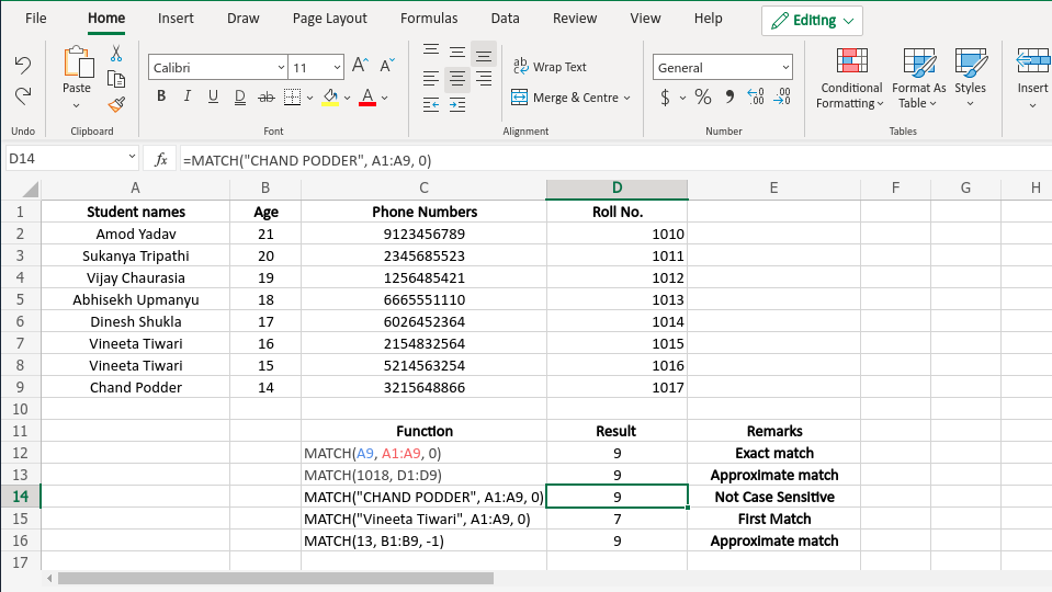
Output Screenshot

Like Article

Save Article

Источник

The MATCH function looks for a specific value and returns its relative position in a given range of cells. The output is the first position found for the given value. Being a lookup and reference function, it works for both an exact and approximate match. For example, if the range A11:A15 consists of the numbers 2, 9, 8, 14, 32, the formula “MATCH(8,A11:A15,0)” returns 3. This is because the number 8 is at the third position.

In simple words, the MATCH formula is given as follows:

“MATCH(value to be searched, array, exact or approximate match [1, 0 or -1])”

MATCH Function in Excel
- The Syntax of the MATCH Excel Function
- How to use the MATCH Function in Excel? (With Examples)
  - Example #1–Exact Match
  - Example #2–Approximate Match
  - Example #3–Wildcard Character (Partial Match)
  - Example 4–INDEX MATCH
- The Properties of the MATCH Excel Function
- Frequently Asked Questions
- Recommended Articles

The Syntax of the MATCH Excel Function

The syntax of the function is shown in the following image:

The function accepts the following arguments:

Lookup_value: This is the value to be searched in the “lookup_array.”
Lookup_array: This is the array or range of cells where the “lookup_value” is to be searched.
Match_type: This takes the values 1, 0, or -1 depending on the type of match.

For instance, you may want to search a specific word (lookup_value) in the dictionary (lookup_array).

The arguments “lookup_value” and “lookup_array” are mandatory, while “match_type” is optional.

The Values of “Match_Type”

The “match_type” can take any of the following values:

Positive one (1): The function looks for the largest value in the “lookup_array,” which is less than or equal to the “lookup_value.” The data is arranged in alphabetical (A to Z) or ascending order and an approximate match is returned.

Zero (0): The function looks for an exact match of the “lookup_value” in the “lookup_array.” The data is not required to be arranged.

Negative one (-1): The function looks for the smallest value in the “lookup_array,” which is greater than or equal to the “lookup_value.” The data is arranged in reverse order of alphabets (Z to A) or descending order and an approximate match is returned.

Note: The default value of “match_type” is 1.

How to use the MATCH Function in Excel? (With Examples)

Let us understand the working of the MATCH formula with the help of examples.

You can download this MATCH Function Excel Template here – MATCH Function Excel Template

Example #1–Exact Match

The succeeding table shows the serial number (S.N.), name, and department of ten employees in an organization. We want to find the position of the employee “Tanuj.”

We apply the following formula.

“=MATCH(F4,$B$4:$B$13,0)”

The “match_type” is set at 0 to return the exact position of “Tanuj” (lookup_value) from the range $B$4:$B$13 (lookup_array). The output is 1.

Example #2–Approximate Match

The succeeding list shows the values from 100 to 1000. We want to find the approximate position of the value 525.

We apply the following formula.

“=MATCH(E19,B19:B28,1)”

The “match_type” is set at 1 to return the approximate match of 525 (lookup_value) from the range B19:B28 (lookup_array).

The MATCH function looks for the largest value (500), which is less than 525 in the given array. Hence, the output is 5.

Example #3–Wildcard Character (Partial Match)

The MATCH function supports the usage of wildcard charactersIn Excel, wildcards are the three special characters asterisk, question mark, and tilde. Asterisk denotes multiple characters, a question mark denotes a single character, and a tilde denotes the identification of a wild card character.read more (? and *) in the “lookup_value” argument. Let us consider an example of the same.

The succeeding list shows ten IDs of the various employees of an organization. We want to find the position of the ID ending with 105.

We apply the following formula.

“=MATCH(“*”&E33,$B$33:$B$42,0)”

The wildcard characters are used for partial matches and the “match_type” is set at zero. The output is 5. This implies that the ID at the fifth position is ending with 105.

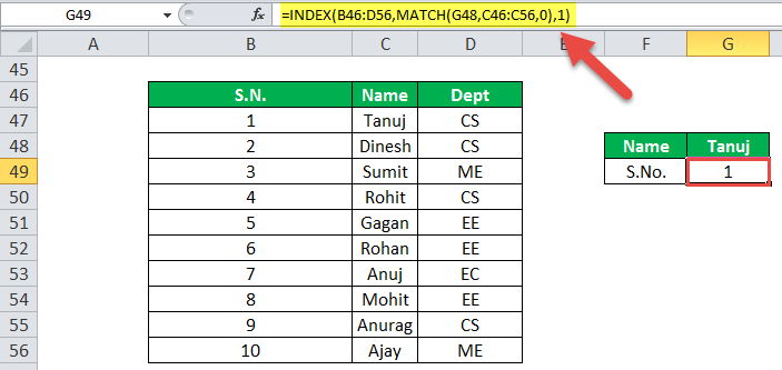
Example 4–INDEX MATCH

The MATCH and INDEX functionThe INDEX function can return the result from the row number, and the MATCH function can give us the position of the lookup value in the array. This combination of the INDEX MATCH is beneficial in addressing a fundamental limitation of VLOOKUP.read more are used together to look up a value in the table from right to left.

The succeeding table shows the serial number (S.N.), name, and department of ten employees in an organization. We want to find the serial number of the employee “Tanuj.”

We apply the following formula.

“=INDEX(B46:D56,MATCH(G48,C46:C56,0),1)”

The MATCH function searches for the exact word “Tanuj” in the range C46:C56 and returns 2. The output 2 is supplied as the row number to the INDEX functionThe INDEX function in Excel helps extract the value of a cell, which is within a specified array (range) and, at the intersection of the stated row and column numbers.read more. The INDEX function returns the value from the second row and first column of the range B46:D56.

The output of the formula is 1. This implies that the serial number of “Tanuj” is 1.

The following image shows the output when the “lookup_value” is “Tanujh.” Since “Tanujh” could not be found in column B, the outcome is “#N/A” error.

The Properties of the MATCH Excel Function

It is not case-sensitive which implies that it does not distinguish between the uppercase and lowercase letters.
It returns the relative position of the “lookup_value” in the “lookup_array.”
It works with one-dimensional ranges or arrays which can be either vertical or horizontal.
If there are multiple occurrences of the “lookup_value” in the “lookup_array,” it returns the position of the first exact match.
If the “lookup_value” is in text form, the wildcard characters like a question mark (?) and asterisk (*) can be used for partial matches.
It returns the “#N/A” error if it is unable to find the “lookup_value” in the “lookup_array.”

Frequently Asked Questions

1. Define the MATCH function of Excel.

The MATCH function returns the position of a given value from a vertical or horizontal array or range of cells. It returns both approximate and exact matches from unsorted and sorted data lists respectively.

The MATCH function can be used in combination with the INDEX function to extract a value from the position supplied by the former. The MATCH function accepts the arguments “lookup_value,” “lookup_array,” and “match_type.”

The first two arguments are mandatory, while the last is optional. The “match_type” can take the values 1, 0 or -1 depending on the type of match. The value 0 refers to an exact match, while 1 and -1 refer to an approximate match.

2. How is the MATCH function used to compare two columns in Excel?

The MATCH function is used in combination with the IF and ISNA functions to compare two columns. The formula is stated as follows:

“IF(ISNA(MATCH(first value in list1,list2,0)),“not in list 1”,“”)”

The formula looks for a value of “list 1” in “list 2.” If it is able to find a value, its relative position is returned. However, if a value of “list 2” is not present in “list 1,” the formula returns the text “not in list 1.”

3. What is the INDEX MATCH formula of Excel?

The INDEX MATCH formula uses a combination of the INDEX and MATCH functions. The INDEX function looks for a value in an array based on the specified row and column numbers. These row and column numbers are supplied by the MATCH function.

The INDEX MATCH formula for a vertical lookup is stated as follows:

“INDEX(column to return a value from,MATCH(lookup_value,column to look up against,0)”

The “column to return a value from” is the “array” argument of the INDEX function. The “column to look up against” is the “lookup_array” argument of the MATCH function.

Note: The “array” argument of the INDEX function must contain the same number of rows as the “lookup_array” argument of the MATCH function.

Syntax

Example

Need more help?

Want more options?

Match type information

Exact match

Approximate match

Wildcard match

INDEX and MATCH

Case-sensitive match

Notes

Что возвращает функция

Синтаксис

Аргументы функции

Дополнительная информация

Примеры использования функции ПОИСКПОЗ в Excel

Table of contents

The Syntax of the MATCH Excel Function

How to use the MATCH Function in Excel? (With Examples)

Example #1–Exact Match

Example #2–Approximate Match

Example #3–Wildcard Character (Partial Match)

Example 4–INDEX MATCH

The Properties of the MATCH Excel Function

Frequently Asked Questions

Recommended Articles