Tip: Try using the new XLOOKUP and XMATCH functions, improved versions of the functions described in this article. These new functions work in any direction and return exact matches by default, making them easier and more convenient to use than their predecessors.
Suppose that you have a list of office location numbers, and you need to know which employees are in each office. The spreadsheet is huge, so you might think it is challenging task. It’s actually quite easy to do with a lookup function.
The VLOOKUP and HLOOKUP functions, together with INDEX and MATCH, are some of the most useful functions in Excel.
Note: The Lookup Wizard feature is no longer available in Excel.
Here’s an example of how to use VLOOKUP.
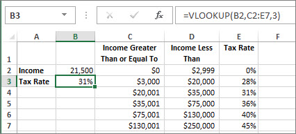
=VLOOKUP(B2,C2:E7,3,TRUE)
In this example, B2 is the first argument—an element of data that the function needs to work. For VLOOKUP, this first argument is the value that you want to find. This argument can be a cell reference, or a fixed value such as «smith» or 21,000. The second argument is the range of cells, C2-:E7, in which to search for the value you want to find. The third argument is the column in that range of cells that contains the value that you seek.
The fourth argument is optional. Enter either TRUE or FALSE. If you enter TRUE, or leave the argument blank, the function returns an approximate match of the value you specify in the first argument. If you enter FALSE, the function will match the value provide by the first argument. In other words, leaving the fourth argument blank—or entering TRUE—gives you more flexibility.
This example shows you how the function works. When you enter a value in cell B2 (the first argument), VLOOKUP searches the cells in the range C2:E7 (2nd argument) and returns the closest approximate match from the third column in the range, column E (3rd argument).
The fourth argument is empty, so the function returns an approximate match. If it didn’t, you’d have to enter one of the values in columns C or D to get a result at all.
When you’re comfortable with VLOOKUP, the HLOOKUP function is equally easy to use. You enter the same arguments, but it searches in rows instead of columns.
Using INDEX and MATCH instead of VLOOKUP
There are certain limitations with using VLOOKUP—the VLOOKUP function can only look up a value from left to right. This means that the column containing the value you look up should always be located to the left of the column containing the return value. Now if your spreadsheet isn’t built this way, then do not use VLOOKUP. Use the combination of INDEX and MATCH functions instead.
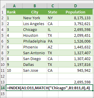
This example shows a small list where the value we want to search on, Chicago, isn’t in the leftmost column. So, we can’t use VLOOKUP. Instead, we’ll use the MATCH function to find Chicago in the range B1:B11. It’s found in row 4. Then, INDEX uses that value as the lookup argument, and finds the population for Chicago in the 4th column (column D). The formula used is shown in cell A14.
For more examples of using INDEX and MATCH instead of VLOOKUP, see the article https://www.mrexcel.com/excel-tips/excel-vlookup-index-match/ by Bill Jelen, Microsoft MVP.
Give it a try
If you want to experiment with lookup functions before you try them out with your own data, here’s some sample data.
VLOOKUP Example at work
Copy the following data into a blank spreadsheet.
Tip: Before you paste the data into Excel, set the column widths for columns A through C to 250 pixels, and click Wrap Text (Home tab, Alignment group).
|
Density |
Viscosity |
Temperature |
|
0.457 |
3.55 |
500 |
|
0.525 |
3.25 |
400 |
|
0.606 |
2.93 |
300 |
|
0.675 |
2.75 |
250 |
|
0.746 |
2.57 |
200 |
|
0.835 |
2.38 |
150 |
|
0.946 |
2.17 |
100 |
|
1.09 |
1.95 |
50 |
|
1.29 |
1.71 |
0 |
|
Formula |
Description |
Result |
|
=VLOOKUP(1,A2:C10,2) |
Using an approximate match, searches for the value 1 in column A, finds the largest value less than or equal to 1 in column A which is 0.946, and then returns the value from column B in the same row. |
2.17 |
|
=VLOOKUP(1,A2:C10,3,TRUE) |
Using an approximate match, searches for the value 1 in column A, finds the largest value less than or equal to 1 in column A, which is 0.946, and then returns the value from column C in the same row. |
100 |
|
=VLOOKUP(0.7,A2:C10,3,FALSE) |
Using an exact match, searches for the value 0.7 in column A. Because there is no exact match in column A, an error is returned. |
#N/A |
|
=VLOOKUP(0.1,A2:C10,2,TRUE) |
Using an approximate match, searches for the value 0.1 in column A. Because 0.1 is less than the smallest value in column A, an error is returned. |
#N/A |
|
=VLOOKUP(2,A2:C10,2,TRUE) |
Using an approximate match, searches for the value 2 in column A, finds the largest value less than or equal to 2 in column A, which is 1.29, and then returns the value from column B in the same row. |
1.71 |
HLOOKUP Example
Copy all the cells in this table and paste it into cell A1 on a blank worksheet in Excel.
Tip: Before you paste the data into Excel, set the column widths for columns A through C to 250 pixels, and click Wrap Text (Home tab, Alignment group).
|
Axles |
Bearings |
Bolts |
|
4 |
4 |
9 |
|
5 |
7 |
10 |
|
6 |
8 |
11 |
|
Formula |
Description |
Result |
|
=HLOOKUP(«Axles», A1:C4, 2, TRUE) |
Looks up «Axles» in row 1, and returns the value from row 2 that’s in the same column (column A). |
4 |
|
=HLOOKUP(«Bearings», A1:C4, 3, FALSE) |
Looks up «Bearings» in row 1, and returns the value from row 3 that’s in the same column (column B). |
7 |
|
=HLOOKUP(«B», A1:C4, 3, TRUE) |
Looks up «B» in row 1, and returns the value from row 3 that’s in the same column. Because an exact match for «B» is not found, the largest value in row 1 that is less than «B» is used: «Axles,» in column A. |
5 |
|
=HLOOKUP(«Bolts», A1:C4, 4) |
Looks up «Bolts» in row 1, and returns the value from row 4 that’s in the same column (column C). |
11 |
|
=HLOOKUP(3, {1,2,3;»a»,»b»,»c»;»d»,»e»,»f»}, 2, TRUE) |
Looks up the number 3 in the three-row array constant, and returns the value from row 2 in the same (in this case, third) column. There are three rows of values in the array constant, each row separated by a semicolon (;). Because «c» is found in row 2 and in the same column as 3, «c» is returned. |
c |
INDEX and MATCH Examples
This last example employs the INDEX and MATCH functions together to return the earliest invoice number and its corresponding date for each of five cities. Because the date is returned as a number, we use the TEXT function to format it as a date. The INDEX function actually uses the result of the MATCH function as its argument. The combination of the INDEX and MATCH functions are used twice in each formula – first, to return the invoice number, and then to return the date.
Copy all the cells in this table and paste it into cell A1 on a blank worksheet in Excel.
Tip: Before you paste the data into Excel, set the column widths for columns A through D to 250 pixels, and click Wrap Text (Home tab, Alignment group).
|
Invoice |
City |
Invoice Date |
Earliest invoice by city, with date |
|
3115 |
Atlanta |
4/7/12 |
=»Atlanta = «&INDEX($A$2:$C$33,MATCH(«Atlanta»,$B$2:$B$33,0),1)& «, Invoice date: » & TEXT(INDEX($A$2:$C$33,MATCH(«Atlanta»,$B$2:$B$33,0),3),»m/d/yy») |
|
3137 |
Atlanta |
4/9/12 |
=»Austin = «&INDEX($A$2:$C$33,MATCH(«Austin»,$B$2:$B$33,0),1)& «, Invoice date: » & TEXT(INDEX($A$2:$C$33,MATCH(«Austin»,$B$2:$B$33,0),3),»m/d/yy») |
|
3154 |
Atlanta |
4/11/12 |
=»Dallas = «&INDEX($A$2:$C$33,MATCH(«Dallas»,$B$2:$B$33,0),1)& «, Invoice date: » & TEXT(INDEX($A$2:$C$33,MATCH(«Dallas»,$B$2:$B$33,0),3),»m/d/yy») |
|
3191 |
Atlanta |
4/21/12 |
=»New Orleans = «&INDEX($A$2:$C$33,MATCH(«New Orleans»,$B$2:$B$33,0),1)& «, Invoice date: » & TEXT(INDEX($A$2:$C$33,MATCH(«New Orleans»,$B$2:$B$33,0),3),»m/d/yy») |
|
3293 |
Atlanta |
4/25/12 |
=»Tampa = «&INDEX($A$2:$C$33,MATCH(«Tampa»,$B$2:$B$33,0),1)& «, Invoice date: » & TEXT(INDEX($A$2:$C$33,MATCH(«Tampa»,$B$2:$B$33,0),3),»m/d/yy») |
|
3331 |
Atlanta |
4/27/12 |
|
|
3350 |
Atlanta |
4/28/12 |
|
|
3390 |
Atlanta |
5/1/12 |
|
|
3441 |
Atlanta |
5/2/12 |
|
|
3517 |
Atlanta |
5/8/12 |
|
|
3124 |
Austin |
4/9/12 |
|
|
3155 |
Austin |
4/11/12 |
|
|
3177 |
Austin |
4/19/12 |
|
|
3357 |
Austin |
4/28/12 |
|
|
3492 |
Austin |
5/6/12 |
|
|
3316 |
Dallas |
4/25/12 |
|
|
3346 |
Dallas |
4/28/12 |
|
|
3372 |
Dallas |
5/1/12 |
|
|
3414 |
Dallas |
5/1/12 |
|
|
3451 |
Dallas |
5/2/12 |
|
|
3467 |
Dallas |
5/2/12 |
|
|
3474 |
Dallas |
5/4/12 |
|
|
3490 |
Dallas |
5/5/12 |
|
|
3503 |
Dallas |
5/8/12 |
|
|
3151 |
New Orleans |
4/9/12 |
|
|
3438 |
New Orleans |
5/2/12 |
|
|
3471 |
New Orleans |
5/4/12 |
|
|
3160 |
Tampa |
4/18/12 |
|
|
3328 |
Tampa |
4/26/12 |
|
|
3368 |
Tampa |
4/29/12 |
|
|
3420 |
Tampa |
5/1/12 |
|
|
3501 |
Tampa |
5/6/12 |
The Combo of VLOOKUP and MATCH is like a superpower. Well, as we all know VLOOKUP is one of the most popular functions.
Right?
It can help you quickly lookup a value in a column. But when you use it more and more you will realize some problems with it. And, the biggest problem is it’s not dynamic.
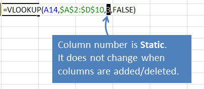
In VLOOKUP, col_index_no is a static value which is the reason VLOOKUP doesn’t work as a dynamic function. And this is where you need to combine VLOOKUP with MATCH.
If you are working on multiple-column data, it’s a pain to change its reference you have to do (change the column number) manually.
The best way to solve this problem is to use the MATCH function in VLOOKUP for col_index_number. Today in this post, I going to explain all the stuff you need to know to use this combo formula.
Problems With VLOOKUP
I have found the two biggest reasons to create a combination of these two functions.
1. Static Reference
Just look at the below data table where you have 12-month sales for four different employees.

Now, let’s say you want to look up the Feb month’s sale of “John”. The formula should be like this.
=VLOOKUP("May",A1:E13,2,0)And in this formula, you have mentioned 2 as the col_index_num because John’s sale is in the second column. But what will you do if your boss tells you to get the sales value for “Peter”?
You need to change the value in col_index_num because it’s not dynamic.
2. Add or Delete Columns
Now think in a different way. You need to add a new column for a new employee just before John’s column.
And here, John’s column number is 3 and your formula result is incorrect.

Again here, because col_index_num is a static value you need to change it manually from 2 to 3 and again if you need something else.
At this point, you are clear about one thing you need to make col_index_num dynamic. And for this, the best way is to replace it with the MATCH function.
Why Match Function
Before you combine VLOOKUP and MATCH, you need to understand the match function and its work. The basic use of MATCH is to find the cell number of the lookup value from a range.
Syntax: MATCH(lookup_value,lookup_array,[match_type])
It has mainly three arguments, lookup value, a range to lookup for the value, and the match type to specify an exact match or an approximate match.
For example, in the below data, I am lookup for the name “John” with the match function from a heading row.

And, it has returned 2 in the result because the name is in the 2nd cell of the row.
VLOOKUP and MATCH Together
Now, it’s time to put VLOOKUP and MATCH together. So, let’s continue with our previous example.
First of all, let’s create a formula by using both of the functions, and then we’ll understand how these two work together.
Steps to create this combo formula:
- First of all, in one cell enter the month’s name, and in another cell enter the employee’s name.
- After that, enter the below formula in the third cell.
=VLOOKUP(C15,A1:E13,MATCH(C16,A1:E1,0),0)
In the above formula, you have used VLOOKUP to lookup for the MAY month, and for the col_index_num argument, you have used the match function instead of a static value.
And in the match function, you have used “John” (employee name) for the lookup value.

Here match function has returned the cell number for the “John” from the above row. After that, VLOOKUP used that cell number to return the value.
In simple words, the MATCH function tells VLOOKUP the column number to get the value from.
Problems Solved?
Above you have learned about two different problems which are because of static col_index_num.
And, for this, you have combined VLOOKUP and MATCH. Now, we need to check whether those problems are solved or not.
1. Static Reference
You have referred to the employee name in the match function to get the column number for VLOOKUP.
When you change the employee name in the cell, the match function will change the column number. And when you need to get the value for a different employee you have to change the employee name in the cell.
This way, you have a dynamic col_index_number.
Finally, you don’t have to edit the formula again and again.
2. Add or Delete Columns
Before adding a new column John’s data was in the 2nd column and the match function returned 2. And after you have inserted a new column john’s data is in the 3rd column and the match returned 3.
When you add a new column for a new employee the value in the formula is not changed because the match function updates its value.
In this way, you’ll always get the correct column number even when you insert/delete any column. The MATCH function will return the right column number.
- Sample-File

VLOOKUP and INDEX-MATCH formulas are among the most powerful functions in Excel. Lookup formulas come in handy whenever you want to have Excel automatically return the price, product ID, address, or some other associated value from a table based on some lookup value. The VLOOKUP function can be used when the lookup value is in the left column of your table or when you want to return the last value in a column. The INDEX and MATCH functions can be used in combination to do the same thing, but provide greater flexibility without some of the limitations of VLOOKUP. I’ll also mention LOOKUP and CHOOSE and EXACT and ISBLANK and ISNUMBER and ISTEXT and … 🙂, but this article is mainly about VLOOKUP and INDEX-MATCH.
To see these examples in action, download the Excel file below.
Download the Example File (LookupFormulas.xlsx)
Do you have a VLOOKUP or INDEX-MATCH challenge you need to solve? If you can’t figure it out after reading this article, go ahead and ask your question by commenting below.
This Article (bookmarks):
- Simple VLOOKUP and INDEX-MATCH Examples
- Wildcard Characters for Partial Match Lookups
- Approximate Match Lookups (for Grades, Discounts, Taxes, etc.)
- 2D Lookups Using VLOOKUP-MATCH and INDEX-MATCH-MATCH
- 3D Lookups Using INDEX-MATCH and VLOOKUP
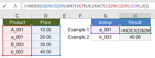
- Case-Sensitive EXACT Lookup Using INDEX-MATCH
- Multiple-Criteria Exact Lookups Using VLOOKUP and INDEX-MATCH
- Lookups with Multiple Non-Exact Criteria Using INDEX-MATCH
- Return the Last Numeric Value in a Column
- Return the Last Text Value in a Column
- Return the Last Non-BLANK Value in a Range
- Return the Last Non-Empty Value in a Range
- Lookup based on the Nth Match
1) Simple VLOOKUP and INDEX-MATCH Examples
VLOOKUP Example
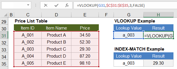
First, here is an example of the VLOOKUP function using a simple Price List Table. We’re looking for the text «a_003» within the Item ID column and wanting to return the corresponding value from the Price column.
=VLOOKUP(lookup_value,table_array,col_index_num,FALSE)
How it works: The table_array argument is a range that must have the lookup column on the left. The price column is the 3rd column in the highlighted range, so that is why the col_index_num argument is 3 in our example. We use FALSE for the final argument because we want the VLOOKUP function to do an exact match.
NOTES Actually, this lookup is not truly «exact» because both VLOOKUP and MATCH are not case-sensitive, but the syntax tooltip in Excel calls the option an «exact match» so we’ll just accept that and explain how to do a case-sensitive match later.
If you later insert a column in the middle of your table_array, the Price column might not be column 3 any more. To prevent your VLOOKUP formula from breaking, in place of the 3 in the example, you can use (COLUMN($E$30)-COLUMN($C$30)+1).
The default for VLOOKUP is not an exact match, so don’t forget to include FALSE as the 4th argument if you want an exact match.
INDEX-MATCH Example
Next, you’ll see that the INDEX-MATCH formula is just as simple:
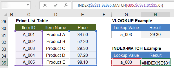
=INDEX(result_range,MATCH(lookup_value,lookup_range,0))
How it works: The MATCH function returns the position number 3 because «a_003» matches the 3rd row in the Item ID range. Next, INDEX(result_range,3) returns the 3rd value in the price list range.
The INDEX-MATCH formula is an example of a simple nested function where we use the result from the MATCH function as one of the arguments for the INDEX function. The example below shows this being done in two separate steps.
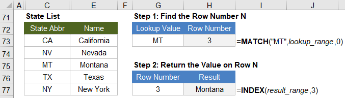
Syntax and Notes for MATCH and INDEX
MATCH returns the position number of a matched value within the lookup range.
=MATCH(lookup_value,lookup_range,match_type)
NOTES When using MATCH, the lookup_range can be a row or column, but if lookup_range is more than one row or column, MATCH will return an error.
MATCH returns the #N/A error when it does not find a match.
The match_type is optional, but the default is not 0. So, it is is best to always specify the match type.
INDEX returns a value from an array based on a row and column number.
=INDEX(array,row_number,[column_number],[area_number])
NOTES You don’t need to include the optional column_number if the array is a single column.
The optional area_number argument is only used for 3D arrays.
If your array is a row, don’t use the shortcut =INDEX(array,column_number) because that may not be compatible with other spreadsheet software. Use =INDEX(array,1,column_number) instead.
2) Use Wildcard Characters (?, *) for Partial Matches with VLOOKUP and INDEX-MATCH
Wildcard characters can be used within the lookup_value for both VLOOKUP and MATCH formulas when the lookup is text and you are doing an exact match.
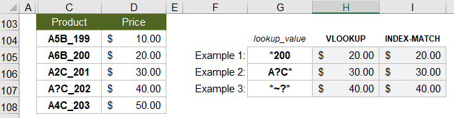
* (asterisk) matches any number of characters. For example, use «*200» to find the first value ending in 200.
? (question mark) matches any single character. For example, use «A?C*» to find the first value where «A» is the first character and «C» is the 3rd character. The second character can be anything, but only a single character.
~ (tilde) is used in front of a wildcard character to treat it as a literal character. In the 3rd example, we use «*~?*» to find the first occurrence of a product that contains an actual question mark.
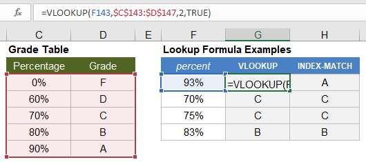
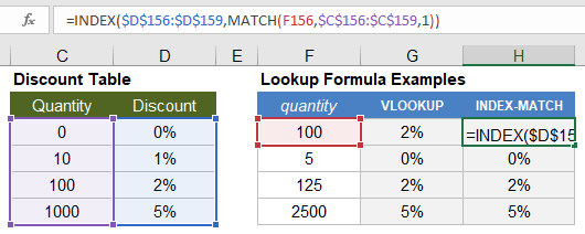
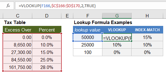
3) Return Approximate Matches Using VLOOKUP and INDEX-MATCH
The following examples show how to use VLOOKUP and INDEX-MATCH to return approximate matches with numerical lookup data. Important: When using an «Approximate Match» with VLOOKUP (where the 4th argument = TRUE) and a «Less than» match with MATCH (where the 3rd argument = 1), the lookup range needs to be sorted in ascending order.
These formulas look for the largest value that is less than or equal to the lookup value.
=VLOOKUP(lookup_value,table_array,col_index_num,TRUE)
=INDEX(result_range,MATCH(lookup_value,lookup_range,1))
Example 1: Return a Grade based on Percent
► See this in action: Download the Grade book Template
Example 2: Return a Discount Rate based on Quantity
Example 3: Return a Tax Rate based on Income
► See this in action: Download the Paycheck Calculator
CAUTION For an approximate match, these formulas use a very efficient search algorithm that assumes the lookup range is sorted in ascending order. If your data is not sorted, they don’t return an error value, but the result may be unpredictable.
If the lookup value is less than the first value in the lookup range, MATCH and VLOOKUP will return an error.
4) 2D Lookups Using VLOOKUP-MATCH and INDEX-MATCH-MATCH
In this example, we’ll do a mileage lookup between two cities. The formulas are basically the same as for a 1D lookup, except that we use a MATCH function to replace col_index_num in the VLOOKUP function and to replace column_number in the INDEX function.
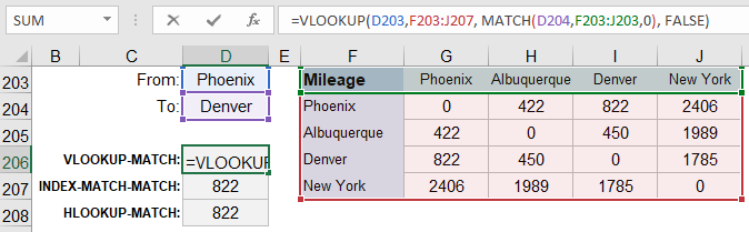
Using VLOOKUP
=VLOOKUP(row_lookup_value,table_array, MATCH(column_lookup_value,column_label_range,0), FALSE)
Using INDEX-MATCH-MATCH
=INDEX( result_array,
MATCH(row_lookup_value,row_label_range,0),
MATCH(column_lookup_value,column_label_range,0) )
Using HLOOKUP
=HLOOKUP(column_lookup_value,table_array, MATCH(row_lookup_value,row_label_range,0), FALSE)
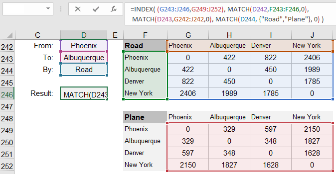
5) 3D Lookups Using INDEX-MATCH and VLOOKUP
To demonstrate a 3D lookup, we’ll use mileage tables again, but this time we have a separate table for Road and Plane. The INDEX function allows you to return a value from a 3D array. You can replace the row_number, column_number, and area_number with 3 MATCH functions.
NOTE The reference argument for the INDEX function should be multiple same-size ranges surrounded by parentheses like this: (A1:D10,E1:H10), or you can use a named range.
=INDEX( (array_range1,array_range2) ,
MATCH(row_lookup_value,row_label_range,0),
MATCH(column_lookup_value,column_label_range,0),
MATCH(table_lookup_value,{"Road","Plane"},0) )
3D Lookup Using VLOOKUP
It is possible to do a 3D lookup using VLOOKUP. Starting with the 2D lookup formula, in place of array_table, you can use CHOOSE(table_number,table_array_1,table_array_2). You can use MATCH to find the value for table_number as in the INDEX-MATCH example above. The resulting formula would look like this:
=VLOOKUP(row_lookup_value, CHOOSE( MATCH(table_name,{"Road","Plane"},0), road_table_array, plane_table_array), MATCH(column_lookup_value,column_label_range,0), FALSE)
6) Case-Sensitive EXACT Lookup Using INDEX-MATCH
Most lookups and logical comparisons in Excel are NOT case-sensitive, meaning that both «A»=»a» and «A»=»A» would return TRUE.
The EXACT(value1,value2) function allows you to make a comparison between value1 and value2 that IS case sensitive, so EXACT(«A»,»a») returns FALSE and EXACT(«B»,»B») returns TRUE.
If you use EXACT to compare a value to a range like EXACT(«B»,A1:A20), the function returns an array of TRUE and FALSE values. You can then use a MATCH function to look for the value TRUE within the range returned by EXACT(lookup_value,lookup_range). The final lookup formula is an Excel Array Formula, so you need to press Ctrl+Shift+Enter after entering the formula.
{Ctrl+Shift+Enter} =INDEX(result_range, MATCH(TRUE,EXACT(lookup_value,lookup_range),0) )
See the references at the end of this article if you are curious about how a case-sensitive lookup can be done with VLOOKUP.
7) Multiple-Criteria Exact Lookups Using VLOOKUP and INDEX-MATCH
One way to do an exact-match using multiple criteria is to concatenate the lookup columns and do a lookup using the concatenated lookup values. VLOOKUP requires using a helper column containing the concatenated lookup columns. INDEX-MATCH does not need the helper column, but it becomes an array formula (Ctrl+Shift+Enter).
Multiple-criteria lookup using VLOOKUP and a helper column
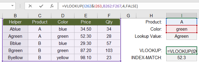
=VLOOKUP(value_1 & value_2,table_array,col_index_num,FALSE)
Multiple-criteria lookup using INDEX-MATCH as an array formula
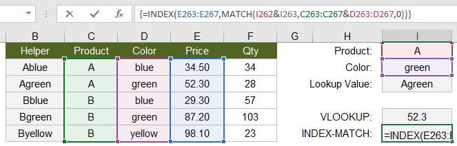
{Ctrl+Shift+Enter} =INDEX(result_range,MATCH(value1 & value2, lookup_col1 & lookup_col2,0))
 Lookups with Multiple Non-Exact Criteria Using INDEX-MATCH
 Lookups with Multiple Non-Exact Criteria Using INDEX-MATCH
When you want to use logical conditions such as A > B or A < B in your lookup, a method I like is to use INDEX-MATCH and convert the lookup_range to a TRUE or FALSE expression like lookup_range<lookup_value. Then search for the first occurrence of TRUE (using 1 as the first argument of the MATCH function). Using this method, you can have any number of conditions because multiplying true/false expressions together acts like the logical AND operator. The formula must be entered as an array formula (Ctrl+Shift+Enter), but that’s a small price to pay for relative simplicity.
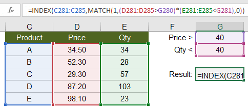
{Ctrl+Shift+Enter} =INDEX(result_range,MATCH(1, (lookup_col1>lookup_value1) * (lookup_col2<lookup_value2) ,0) )
9) Return the Last Numeric Value in a Column
When using an approximate lookup for VLOOKUP and MATCH, you can return the last numeric value in a column if you use an extremely large number as the lookup value (to make sure it will be larger than any number in the lookup range). A common example would be to return the last value in a Balance column for a checkbook register as shown in the example below.
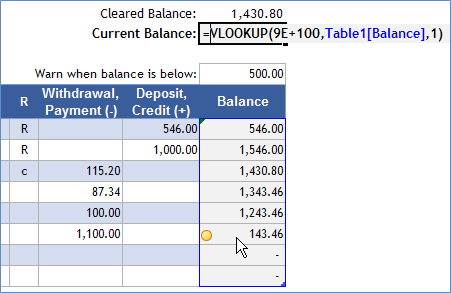
=VLOOKUP( 9E+100, lookup_column, 1, TRUE)
Recall that the TRUE option (for an approximate match) is the default for VLOOKUP, so that is why the formula in the checkbook example image only shows 3 arguments.
This can of course be done with INDEX-MATCH, but I prefer the VLOOKUP formula in this case because it requires only one reference to the lookup column.
=INDEX( lookup_column, MATCH( 9E+99, lookup_column, 1) )
NOTES The lookup_column can contain text values and even errors (like #N/A or #DIV/0), and those values will be ignored. The formula returns only the last numeric value.
10) Return the Last Text Value in a Column
When searching for the last text value, instead of a large numeric value for the lookup_value as in the previous example, use a «large» text value. By that, I mean a text value that would show up last if you sorted a column in alphabetical order. If you are using the English alphabet without special characters, that could be «zzzzzz.» If you are using Greek characters or symbols in your list, you could try a Unicode Character such as «🗿» as the lookup value.
=VLOOKUP( "zzzzzzz", lookup_column, 1, TRUE)
=INDEX( lookup_column, MATCH( "🗿", lookup_column, 1) )
Rather than returning the last text value, I often use just the MATCH part of this formula to return the row number of the last value. This allows you to make a dynamic named range that can be used as the source range for a drop-down list via data validation.
11) Return the Last Non-BLANK Value in a Column
If your column contains both text and numeric values, you may want a formula to return the last non-BLANK value. Using the INDEX-MATCH formula, we can search for the last numeric value and the last text value and return whichever comes last.
=INDEX( lookup_column, MAX( MATCH( "zzzzzz", lookup_column, 1), MATCH(9E+100, lookup_column,1) ) )
A more concise formula uses the LOOKUP function. The LOOKUP function allows the lookup_range to be an expression rather than a direct reference (and it can be a row or column). We can use a logical comparison and search for the last TRUE value like this:
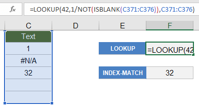
=LOOKUP(42, 1/NOT(ISBLANK(lookup_range)), lookup_range)
The trick here is that the expression 1/NOT(ISBLANK(lookup_range)) returns an array of 1s for TRUE and #DIV/0 errors for FALSE. LOOKUP ignores the error values so it will return the last value in lookup_range that is not blank. The number 42 is arbitrary — it just needs to be larger than 1 to return the last value.
Using very similar formulas, you can use LOOKUP to return just the last numeric value or text value like this:
=LOOKUP( 42, 1/ISNUMBER(lookup_range), result_range)
=LOOKUP( 42, 1/ISTEXT(lookup_range), result_range)
12) Return the Last Non-Empty Value Using LOOKUP
If you are using a formula to return an empty value «» and you want to ignore those cells when searching for the last value in the range, you can use the LOOKUP formula mentioned in the last example with the expression 1/(lookup_range<>»»).
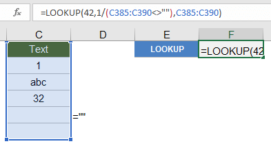
=LOOKUP(42, 1/(lookup_range<>""), lookup_range)
If you want to return the relative row number instead of the actual value, you can use the following formula:
=LOOKUP(42, 1/(lookup_range<>""), ROW(lookup_range)-ROW(first_cell_in_lookup_range)+1 )
13) Lookup based on the Nth Match
You can use the SMALL function to return the Nth smallest value from an array, and we can use that along with an array formula and the INDEX function to do a lookup based on the Nth match. See my Array Formula Examples article to learn more about Array Formulas and specifically the SMALL-IF formula.
In this example, we want to return the 2nd Event that matches the date 3/7/2018. Note: The curly { } brackets in the formula below are a reminder to press Ctrl+Shift+Enter to enter the formula as an Array Formula. You don’t actually type the brackets into the formula.
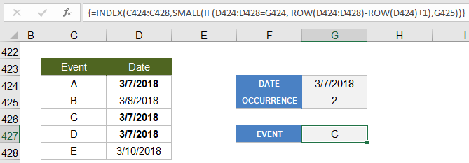
{ =INDEX(result_range,SMALL( IF(lookup_range=lookup_value, ROW(lookup_range)-ROW(first_cell_in_lookup_range)+1),occurrence)) }
How does this work? The SMALL-IF part of the formula is acting kind of like the MATCH function except that it is returning the index number for the 2nd occurrence of the match. We can use SMALL in this example because Excel stores dates as numbers.
This formula is used within the Daily Planner Template to list events and holidays occurring on a particular date.
14) VLOOKUP vs. INDEX-MATCH
Excel people like to debate about whether VLOOKUP is better than INDEX-MATCH for lookup formulas. The most common argument is that VLOOKUP is simpler and INDEX-MATCH is more powerful. Even though I usually prefer INDEX-MATCH, I think both formulas are pretty simple, and one isn’t necessarily always more powerful than the other.
If you want to do more advanced lookups with VLOOKUP, then you’ll probably need to learn how to use MATCH and CHOOSE. If you want to become a power Excel user, then you’ll also want to learn the INDEX function. So, my opinion on the VLOOKUP vs. INDEX-MATCH debate is to learn how to use them all.
In conclusion, here are some reminders applicable to both VLOOKUP and INDEX-MATCH:
- Don’t forget the FALSE or 0 option if you are wanting an exact match, because the default parameter is to use an approximate match.
- As a general rule, use absolute ($A$1) cell references to refer to the lookup ranges and table arrays because when you copy the lookup formula you will usually want those ranges to remain the same.
- Check for extra blank spaces if you think a lookup formula should be finding a match, but it is not.
- Use IFERROR to handle the error returned when an exact match is not found.
References
- Spreadsheet Tips Workbook — vertex42.com — by Jon Wittwer and Brent Weight
- VLOOKUP Function — support.office.com — The official documentation of the VLOOKUP function.
- MATCH Function — support.office.com — The official documentation of the MATCH function.
- INDEX Function — support.office.com — The official documentation of the INDEX function.
- Case-Sensitive Match Using VLOOKUP — at ablebits.com — This shows that it IS possible, but the solution is quite complex.
- Get Value of Last Non-Empty Cell — at exceljet.net — I think this article explains the LOOKUP function better than I did.
This post provides an explanation of how to use the VLOOKUP and MATCH functions to give you better control over how the column index number changes. This is often referred to as a dynamic formula. You will learn how this dynamic duo can help prevent errors and improve your VLOOKUP formulas.

We are going to learn how the MATCH function can be used inside the VLOOKUP function. This helps protect the VLOOKUP from returning errors when changes are made to the workbook.
Problems with VLOOKUPs
The VLOOKUP is a very useful function, but it doesn’t respond to change very well. Have you ever noticed that if you add or delete columns in an area that the VLOOKUP refers to, the result can return an error or incorrect result?
This is usually due to the fact that we have specified the column number as a static number in the 3rd argument of the VLOOKUP argument.
The Starbucks Menu Example
We can use the Starbucks menu VLOOKUP example to help explain this issue.
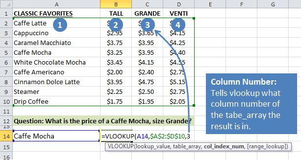
In that example we wanted to return the price for the size Grande, which was in column 3 of the menu. We put a “3” in the column index argument in the VLOOKUP formula to reference the Grande column (col C).
But what if Starbucks decided to add a new size to the menu?
Let’s say they decide to add a size “Short” to the menu, and put it to the left of the size Tall.
In our spreadsheet example, we would need to insert a column after column A for the new size. This change means that the size Grande is now in column 4 (col D).
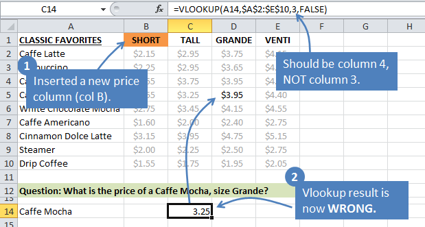
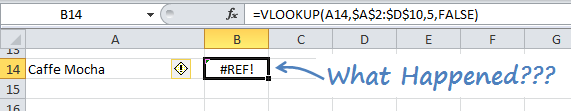
However, our VLOOKUP still references column 3. Excel does NOT update the formula when a column is inserted or deleted.
Therefore, the formula is now returning the wrong result.
This is a problem! But fortunately for us, VLOOKUP has a side-kick named MATCH that will save the day.
MATCH to the Rescue
We first need to learn how the MATCH function works.
The MATCH function is very similar to the VLOOKUP. It’s job is to look through a range of cells and find a match.
The difference is that it returns a row or column number.
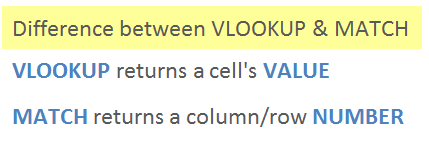
So why the Batman and Robin reference?
I like to think of MATCH as VLOOKUP’s little brother, or side-kick. They do very similar jobs, but MATCH packs a smaller punch.
Batman is the VLOOKUP and returns a big value in the form of a cell’s value. This can be text or a number.
Robin is the MATCH and returns a smaller value in the form of a number.

Hopefully this will help you remember and distinguish the difference between the two.
The Match Function Components
The MATCH function’s arguments are similar to the VLOOKUP’s. The following image shows the Excel definition of the VLOOKUP function, and then my simple definition. This simple definition just makes it easier for me to remember the three arguments.
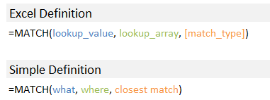
I explain this simple definition below as we walk through an example of creating a VLOOKUP formula.
The MATCH Example
Let’s look at the Starbucks menu example again to learn MATCH. In this example we want to use the MATCH function to return the column number for the size Grande.
I’ll explain why later, but for now we just want to answer the question:
“What is the column number for the size Grande?”
We will answer this question using the MATCH function. You can download the file to follow along.
1. lookup_value – This is the what argument.
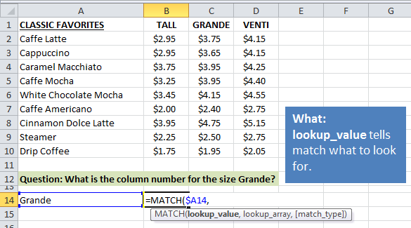
In the first argument we tell the VLOOKUP what we are looking for. In this example we are looking for “Grande” in row 1. I have entered the text “Grande” in cell A14, so we can make a reference to cell A14 in the formula.
2. lookup_array – This is the where argument.
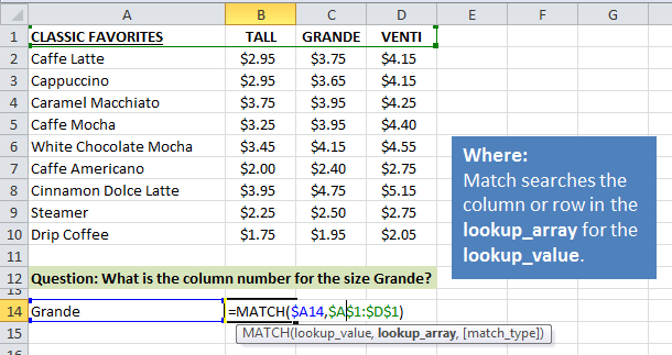
Here we need to tell MATCH where to look for the word “Grande”. I selected the range $A$1:$D$1, which contains the column header names. MATCH will look through row 1 from left-to-right until it finds a match.
You can also specify a column for this argument. In that case MATCH would look down the column from top-to-bottom to find a match.
3. [match_type] – The match type tells MATCH how precise to be with the lookup.
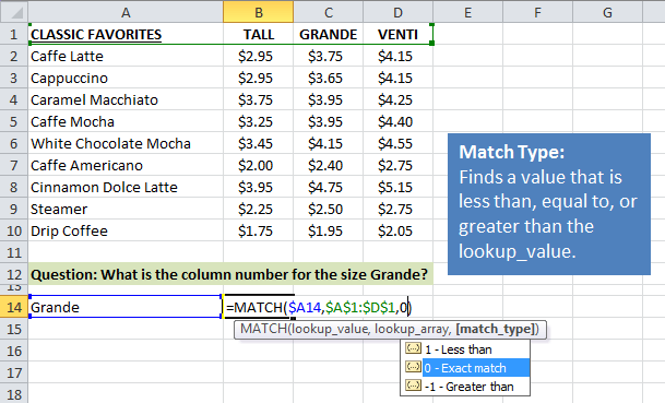
Here we specify if the function should look for an exact MATCH, or a value that is less than or greater than the lookup_value.
In this example we will use “Exact match”, which is represented by putting a 0 (zero) in the third argument. When your MATCH is looking up text you will generally want to look for an exact match.
If you are looking up numbers with the MATCH function then the “Less than” or “Greater than” match types can be very useful.
The Result – Grande is in column 3.
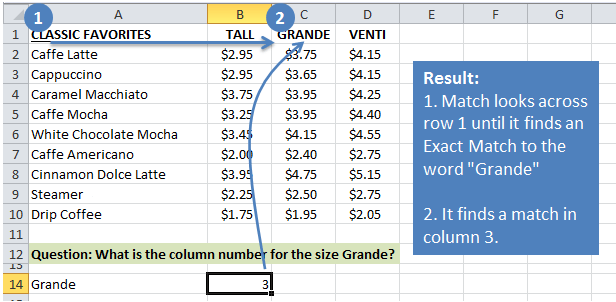
The MATCH function was able to lookup the word “Grande” in row 1 and return the value of 3 in cell B14.
Now let’s see how the MATCH function can be a little more dynamic. In the following screenshot I inserted a column to the left of column B with a new size, “Short”.
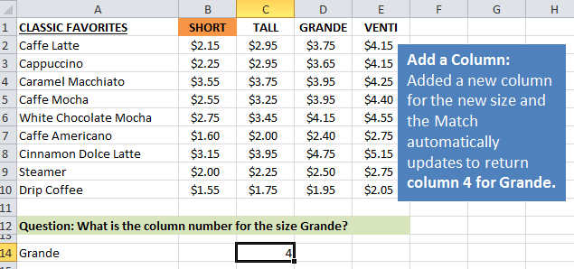
You will notice that the result of the MATCH formula changed to “4”. This is because the word “Grande” is now in the 4th column of the lookup_array (A1:E1).
You are probably starting to see how this could help our original problem of the VLOOKUP returning the wrong result.
VLOOKUP & MATCH – The Dynamic Duo
Now let’s see how we can combine these two to create a dynamic formula.
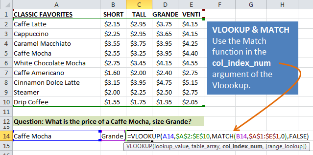
We can use the MATCH function inside the VLOOKUP function. Instead of specifying the column number with a static number “3”, we will use the MATCH function in its place.
Since the MATCH returns a number, it is a perfect fit for the VLOOKUP’s col_index_num argument.
The following example illustrates this. You can follow along in the ‘VLOOKUP & MATCH Example’ sheet in the example file.
The original formula looked like the following:
=VLOOKUP(A14,$A$2:$E$10,4,FALSE)
In the new formula I replace the “4” with the MATCH formula:
=VLOOKUP(A14,$A$2:$E$10,MATCH(B14,$A$1:$E$1,0),FALSE)
The MATCH formula references cell B14, which contains the word “Grande”. The formula looks up the word Grande in row 1 and returns a 4 as the result because Grande is in the fourth column of the range A1:E1.
The VLOOKUP formula is now much more dynamic with MATCH included. We can add or delete columns to the menu (table), and the VLOOKUP will still return the price for the size that is specified in cell B14.
You could also change either the item in cell A14 or the size in cell B14 to return different prices in cell C14.
This makes the formula very flexible, and easier to reuse in other places in the workbook.
Conclusion
I hope this post has helped you understand how the VLOOKUP and MATCH functions can work together to be a dynamic duo. This team of functions will help prevent errors in your formulas. It will also help you create financial models that are more flexible for data retrieval and scenario analysis.
Series: The Lookup Functions Explained
This is the 2nd post in a series about the most commonly used lookup functions in Excel.
- In the first post I explained the VLOOKUP function at Starbucks.
- In this second post I explained how to make lookup formulas more dynamic with the VLOOKUP & MATCH functions.
- In the third post I explain the INDEX function.
Please leave a comment below with any questions or comments.
Return to Excel Formulas List
Download Example Workbook
Download the example workbook
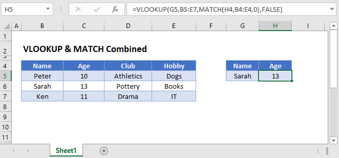
This tutorial will demonstrate how to retrieve data from multiple columns using the MATCH and VLOOKUP Functions in Excel and Google Sheets.
Why Should you Combine VLOOKUP and MATCH?
Traditionally, when using the VLOOKUP Function, you enter a column index number to determine which column to retrieve data from.
This presents two problems:
- If you want to pull values from multiple columns, you must manually enter the column index number for each column
- If you insert or remove columns, your column index number will no longer be valid.
To make your VLOOKUP Function dynamic, you can find the column index number with the MATCH Function.
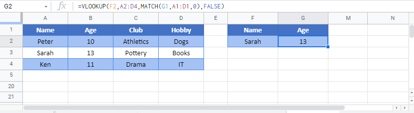
=VLOOKUP(G3,B3:E5,MATCH(H2,B2:E2,0),FALSE)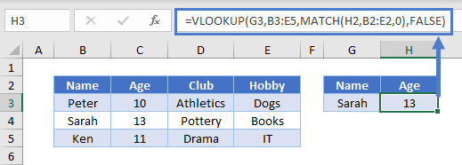
Let’s see how this formula works.
MATCH Function
The MATCH Function will return the column index number of your desired column header.
In the example below, the column index number for “Age” is calculated by the MATCH Function:
=MATCH("Age",B2:E2,0)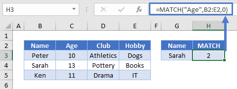
“Age” is the 2nd column header, so 2 is returned.
Note: The last argument of the MATCH Function must be set to 0 to perform an exact match.
VLOOKUP Function
Now, you can simply plug in the result of the MATCH Function into your VLOOKUP Function:
=VLOOKUP(G3,B3:E5,H3,FALSE)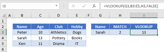
Replacing the column index argument with the MATCH Function gives us our original formula:
=VLOOKUP(G3,B3:E5,MATCH(H2,B2:E2,0),FALSE)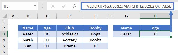
Inserting and Deleting Columns
Now, when you insert or delete columns in the data range, the result of your formula will not change.
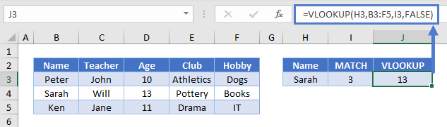
In the example above, we added the Teacher column to the range but still want the student’s Age. The output from the MATCH Function identifies that “Age” is now the 3rd item in the header range, and the VLOOKUP Function uses 3 as the column index.
Locking Cell References
To make our formulas easier to read, we’ve shown the formulas without locked cell references:
=VLOOKUP(G3,B3:E5,MATCH(H2,B2:E2,0),FALSE)But these formulas will not work properly when copy and pasted elsewhere in your file. Instead, you should use locked cell references like this:
=VLOOKUP($G3,$B$3:$E$5,MATCH(H$2,$B$2:$E$2,0),FALSE)Read our article on Locking Cell References to learn more.
VLOOKUP & MATCH Combined in Google Sheets
These formulas work exactly the same in Google Sheets as in Excel.