
Содержание
- Value exists in a range
- Related functions
- Summary
- Generic formula
- Explanation
- COUNTIF function
- Slightly abbreviated
- Testing for a partial match
- An alternative formula using MATCH
- How to use MATCH function in Excel — formula examples
- Excel MATCH function — syntax and uses
- 4 things you should know about MATCH function
- How to use MATCH in Excel — formula examples
- Partial match with wildcards
- Case-sensitive MATCH formula
- Compare 2 columns for matches and differences (ISNA MATCH)
- Excel VLOOKUP and MATCH
- Excel HLOOKUP and MATCH
Value exists in a range
Summary
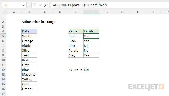
To test if a value exists in a range of cells, you can use a simple formula based on the COUNTIF function and the IF function. In the example shown, the formula in F5, copied down, is:
where data is the named range B5:B16. As the formula is copied down it returns «Yes» if the value in column E exists in B5:B16 and «No» if not.
Generic formula
Explanation
In this example, the goal is to use a formula to check if a specific value exists in a range. The easiest way to do this is to use the COUNTIF function to count occurences of a value in a range, then use the count to create a final result.
COUNTIF function
The COUNTIF function counts cells that meet supplied criteria. The generic syntax looks like this:
Range is the range of cells to test, and criteria is a condition that should be tested. COUNTIF returns the number of cells in range that meet the condition defined by criteria. If no cells meet criteria, COUNTIF returns zero. In the example shown, we can use COUNTIF to count the values we are looking for like this
Once the named range data (B5:B16) and cell E5 have been evaluated, we have:
COUNTIF returns 1 because «Blue» occurs in the range B5:B16 once. Next, we use the greater than operator (>) to run a simple test to force a TRUE or FALSE result:
By itself, the formula above will return TRUE or FALSE. The last part of the problem is to return a «Yes» or «No» result. To handle this, we nest the formula above into the IF function like this:
This is the formula shown in the worksheet above. As the formula is copied down, COUNTIF returns a count of the value in column E. If the count is greater than zero, the IF function returns «Yes». If the count is zero, IF returns «No».
Slightly abbreviated
It is possible to shorten this formula slightly and get the same result like this:
Here, we have remove the «>0» test. Instead, we simply return the count to IF as the logical_test. This works because Excel will treat any non-zero number as TRUE when the number is evaluated as a Boolean.
Testing for a partial match
To test a range to see if it contains a substring (a partial match), you can add a wildcard to the formula. For example, if you have a value to look for in cell C1, and you want to check the range A1:A100 for partial matches, you can configure COUNTIF to look for the value in C1 anywhere in a cell by concatenating asterisks on both sides:
The asterisk (*) is a wildcard for one or more characters. By concatenating asterisks before and after the value in C1, the formula will count the text in C1 anywhere it appears in each cell of the range. To return «Yes» or «No», nest the formula inside the IF function as above.
An alternative formula using MATCH
As an alternative, you can use a formula that uses the MATCH function with the ISNUMBER function instead of COUNTIF:
The MATCH function returns the position of a match (as a number) if found, and #N/A if not found. By wrapping MATCH inside ISNUMBER, the final result will be TRUE when MATCH finds a match and FALSE when MATCH returns #N/A.
Источник
How to use MATCH function in Excel — formula examples
 by Svetlana Cheusheva, updated on March 20, 2023
This tutorial explains how to use MATCH function in Excel with formula examples. It also shows how to improve your lookup formulas by a making dynamic formula with VLOOKUP and MATCH.
In Microsoft Excel, there are many different lookup/reference functions that can help you find a certain value in a range of cells, and MATCH is one of them. Basically, it identifies a relative position of an item in a range of cells. However, the MATCH function can do much more than its pure essence.
Excel MATCH function — syntax and uses
The MATCH function in Excel searches for a specified value in a range of cells, and returns the relative position of that value.
The syntax for the MATCH function is as follows:
Lookup_value (required) — the value you want to find. It can be a numeric, text or logical value as well as a cell reference.
Lookup_array (required) — the range of cells to search in.
Match_type (optional) — defines the match type. It can be one of these values: 1, 0, -1. The match_type argument set to 0 returns only the exact match, while the other two types allow for approximate match.
- 1 or omitted (default) — find the largest value in the lookup array that is less than or equal to the lookup value. Requires sorting the lookup array in ascending order, from smallest to largest or from A to Z.
- 0 — find the first value in the array that is exactly equal to the lookup value. No sorting is required.
- -1 — find the smallest value in the array that is greater than or equal to the lookup value. The lookup array should be sorted in descending order, from largest to smallest or from Z to A.
To better understand the MATCH function, let’s make a simple formula based on this data: students names in column A and their exam scores in column B, sorted from largest to smallest. To find out where a specific student (say, Laura) stands among others, use this simple formula:
=MATCH(«Laura», A2:A8, 0)
Optionally, you can put the lookup value in some cell (E1 in this example) and reference that cell in your Excel Match formula:
=MATCH(E1, A2:A8, 0) 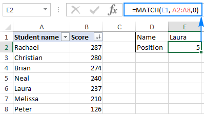
As you see in the screenshot above, the student names are entered in an arbitrary order, and therefore we set the match_type argument to 0 (exact match), because only this match type does not require sorting values in the lookup array. Technically, the Match formula returns the relative position of Laura in the range. But because the scores are sorted from largest to smallest, it also tells us that Laura has the 5 th best score among all students.
Tip. In Excel 365 and Excel 2021, you can use the XMATCH function, which is a modern and more powerful successor of MATCH.
4 things you should know about MATCH function
As you have just seen, using MATCH in Excel is easy. However, as is the case with nearly any other function, there are a few specificities that you should be aware of:
- The MATCH function returns the relative position of the lookup value in the array, not the value itself.
- MATCH is case-insensitive, meaning it does not distinguish between lowercase and uppercase characters when dealing with text values.
- If the lookup array contains several occurrences of the lookup value, the position of the first value is returned.
- If the lookup value is not found in the lookup array, the #N/A error is returned.
How to use MATCH in Excel — formula examples
Now that you know the basic uses of the Excel MATCH function, let’s discuss a few more formula examples that go beyond the basics.
Partial match with wildcards
Like many other functions, MATCH understands the following wildcard characters:
- Question mark (?) — replaces any single character
- Asterisk (*) — replaces any sequence of characters
Note. Wildcards can only be used in Match formulas with match_type set to 0.
A Match formula with wildcards comes useful in situations when you want to match not the entire text string, but only some characters or some part of the string. To illustrate the point, consider the following example.
Supposing you have a list of regional resellers and their sales figures for the past month. You want to find a relative position of a certain reseller in the list (sorted by the Sales amounts in descending order) but you cannot remember his name exactly, though you do remember a few first characters.
Assuming the reseller names are in the range A2:A11, and you are searching for the name that begins with «car», the formula goes as follows:
To make our Match formula more versatile, you can type the lookup value in some cell (E1 in this example), and concatenate that cell with the wildcard character, like this:
As shown in the screenshot below, the formula returns 2, which is the position of «Carter»: 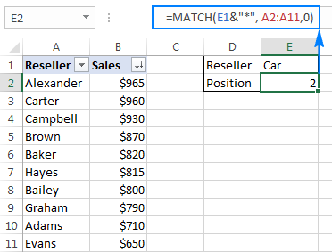
To replace just one character in the lookup value, use the «?» wildcard operator, like this:
The above formula will match the name «Baker» and rerun its relative position, which is 5.
Case-sensitive MATCH formula
As mentioned in the beginning of this tutorial, the MATCH function doesn’t distinguish uppercase and lowercase characters. To make a case-sensitive Match formula, use MATCH in combination with the EXACT function that compares cells exactly, including the character case.
Here’s the generic case-sensitive formula to match data:
The formula works with the following logic:
- The EXACT function compares the lookup value with each element of the lookup array. If the compared cells are exactly equal, the function returns TRUE, FALSE otherwise.
- And then, the MATCH function compares TRUE (which is its lookup_value ) with each value in the array returned by EXACT, and returns the position of the first match.
Please bear in mind that it’s an array formula that requires pressing Ctrl + Shift + Enter to be completed correctly.
Assuming your lookup value is in cell E1 and the lookup array is A2:A9, the formula is as follows:
The following screenshot shows the case-sensitive Match formula in Excel: 
Compare 2 columns for matches and differences (ISNA MATCH)
Checking two lists for matches and differences is one of the most common tasks in Excel, and it can be done in a variety of ways. An ISNA/MATCH formula is one of them:
For any value of List 2 that is not present in List 1, the formula returns «Not in List 1«. And here’s how:
- The MATCH function searches for a value from List 1 within List 2. If a value is found, it returns its relative position, #N/A error otherwise.
- The ISNA function in Excel does only one thing — checks for #N/A errors (meaning «not available»). If a given value is an #N/A error, the function returns TRUE, FALSE otherwise. In our case, TRUE means that a value from List 1 is not found within List 2 (i.e. an #N/A error is returned by MATCH).
- Because it may be very confusing for your users to see TRUE for values that do not appear in List 1, you wrap the IF function around ISNA to display «Not in List 1» instead, or whatever text you want.
For example, to compare values in column B against values in column A, the formula takes the following shape (where B2 is the topmost cell):
=IF(ISNA(MATCH(B2,A:A,0)), «Not in List 1», «»)
As you remember, the MATCH function in Excel is case-insensitive by itself. To get it to distinguish the character case, embed the EXACT function in the lookup_array argument, and remember to press Ctrl + Shift + Enter to complete this array formula:
=IF(ISNA(MATCH(TRUE, EXACT(A:A, B2),0)), «Not in List 1», «»)
The following screenshot shows both formulas in action: 
To learn other ways to compare two lists in Excel, please see the following tutorial: How to compare 2 columns in Excel.
Excel VLOOKUP and MATCH
This example assumes you already have some basic knowledge of Excel VLOOKUP function. And if you do, chances are that you’ve run into its numerous limitations (the detailed overview of which can be found in Why Excel VLOOKUP is not working) and are looking for a more robust alternative.
One of the most annoying drawbacks of VLOOKUP is that it stops working after inserting or deleting a column within a lookup table. This happens because VLOOKUP pulls a matching value based on the number of the return column that you specify (index number). Because the index number is «hard-coded» in the formula, Excel is unable to adjust it when a new column(s) is added to or deleted from the table.
The Excel MATCH function deals with a relative position of a lookup value, which makes it a perfect fit for the col_index_num argument of VLOOKUP. In other words, instead of specifying the return column as a static number, you use MATCH to get the current position of that column.
To make things easier to understand, let’s use the table with students’ exam scores again (similar to the one we used at the beginning of this tutorial), but this time we will be retrieving the real score and not its relative position.
Assuming the lookup value is in cell F1, the table array is $A$1:$C$2 (it’s a good practice to lock it using absolute cell references if you plan to copy the formula to other cells), the formula goes as follows:
=VLOOKUP(F1, $A$1:$C$8, 3, FALSE)
The 3 rd argument (col_index_num) is set to 3 because the Math Score that we want to pull is the 3 rd column in the table. As you can see in the screenshot below, this regular Vlookup formula works well: 
But only until you insert or delete a column(s): 
So, why the #REF! error? Because col_index_num set to 3 tells Excel to get a value from the third column, whereas now there are only 2 columns in the table array.
To prevent such things from happening, you can make your Vlookup formula more dynamic by including the following Match function:
- E2 is the lookup value, which is exactly equal to the name of the return column, i.e. the column from which you want to pull a value (Math Score in this example).
- A1:C1 is the lookup array containing the table headers.
And now, include this Match function in the col_index_num argument of your Vlookup formula, like this:
=VLOOKUP(F1,$A$1:$C$8, MATCH(E2,$A$1:$C$1, 0), FALSE)
And make sure it works impeccably no matter how many columns you add or delete: 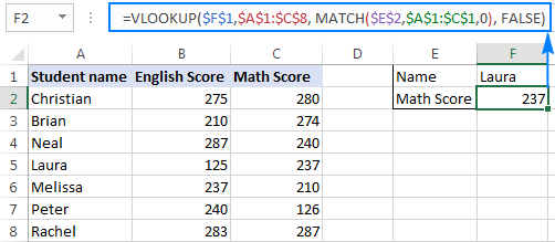
In the screenshot above, I locked all cell references for the formula to work correctly even if my users move it to another place in the worksheet. A you can see in the screenshot below, the formula works just fine after deleting a column; furthermore Excel is smart enough to properly adjust absolute references in this case: 
Excel HLOOKUP and MATCH
In a similar manner, you can use the Excel MATCH function to improve your HLOOKUP formulas. The general principle is essentially the same as in case of Vlookup: you use the Match function to get the relative position of the return column, and supply that number to the row_index_num argument of your Hlookup formula.
Supposing the lookup value is in cell B5, table array is B1:H3, the name of the return row (lookup value for MATCH) is in cell A6 and row headers are A1:A3, the complete formula is as follows:
=HLOOKUP(B5, B1:H3, MATCH(A6, A1:A3, 0), FALSE) 
As you have just seen, the combination of Hlookup/Vlookup & Match is certainly an improvement over regular Hlookup and Vlookup formulas. However, the MATCH function doesn’t eliminate all their limitations. In particular, a Vlookup Match formula still cannot look at its left, and Hlookup Match fails to search in any row other than the topmost one.
To overcome the above (and a few other) limitations, consider using a combination of INDEX MATCH, which provides a really powerful and versatile way to do lookup in Excel, superior to Vlookup and Hlookup in many respects. The detailed guidance and formula examples can be found in INDEX & MATCH in Excel — a better alternative to VLOOKUP.
This is how you use MATCH formulas in Excel. Hopefully, the examples discussed in this tutorial will prove helpful in your work. I thank you for reading and hope to see you on our blog next week!
Источник
MATCH function
Tip: Try using the new XMATCH function, an improved version of MATCH that works in any direction and returns exact matches by default, making it easier and more convenient to use than its predecessor.
The MATCH function searches for a specified item in a range of cells, and then returns the relative position of that item in the range. For example, if the range A1:A3 contains the values 5, 25, and 38, then the formula =MATCH(25,A1:A3,0) returns the number 2, because 25 is the second item in the range.

Tip: Use MATCH instead of one of the LOOKUP functions when you need the position of an item in a range instead of the item itself. For example, you might use the MATCH function to provide a value for the row_num argument of the INDEX function.
Syntax
MATCH(lookup_value, lookup_array, [match_type])
The MATCH function syntax has the following arguments:
-
lookup_value Required. The value that you want to match in lookup_array. For example, when you look up someone’s number in a telephone book, you are using the person’s name as the lookup value, but the telephone number is the value you want.
The lookup_value argument can be a value (number, text, or logical value) or a cell reference to a number, text, or logical value.
-
lookup_array Required. The range of cells being searched.
-
match_type Optional. The number -1, 0, or 1. The match_type argument specifies how Excel matches lookup_value with values in lookup_array. The default value for this argument is 1.
The following table describes how the function finds values based on the setting of the match_type argument.
|
Match_type |
Behavior |
|
1 or omitted |
MATCH finds the largest value that is less than or equal to lookup_value. The values in the lookup_array argument must be placed in ascending order, for example: …-2, -1, 0, 1, 2, …, A-Z, FALSE, TRUE. |
|
0 |
MATCH finds the first value that is exactly equal to lookup_value. The values in the lookup_array argument can be in any order. |
|
-1 |
MATCH finds the smallest value that is greater than or equal tolookup_value. The values in the lookup_array argument must be placed in descending order, for example: TRUE, FALSE, Z-A, …2, 1, 0, -1, -2, …, and so on. |
-
MATCH returns the position of the matched value within lookup_array, not the value itself. For example, MATCH(«b»,{«a»,»b»,»c«},0) returns 2, which is the relative position of «b» within the array {«a»,»b»,»c»}.
-
MATCH does not distinguish between uppercase and lowercase letters when matching text values.
-
If MATCH is unsuccessful in finding a match, it returns the #N/A error value.
-
If match_type is 0 and lookup_value is a text string, you can use the wildcard characters — the question mark (?) and asterisk (*) — in the lookup_value argument. A question mark matches any single character; an asterisk matches any sequence of characters. If you want to find an actual question mark or asterisk, type a tilde (~) before the character.
Example
Copy the example data in the following table, and paste it in cell A1 of a new Excel worksheet. For formulas to show results, select them, press F2, and then press Enter. If you need to, you can adjust the column widths to see all the data.
|
Product |
Count |
|
|
Bananas |
25 |
|
|
Oranges |
38 |
|
|
Apples |
40 |
|
|
Pears |
41 |
|
|
Formula |
Description |
Result |
|
=MATCH(39,B2:B5,1) |
Because there is not an exact match, the position of the next lowest value (38) in the range B2:B5 is returned. |
2 |
|
=MATCH(41,B2:B5,0) |
The position of the value 41 in the range B2:B5. |
4 |
|
=MATCH(40,B2:B5,-1) |
Returns an error because the values in the range B2:B5 are not in descending order. |
#N/A |
Need more help?
For =match() to work, the value of the cells you are referencing have to be exact. Also, the match function only provides the location of the queried term in the search array. So, if you do this right, it will return a value greater than 0, which we can use to our advantage. Your =if() function requires a logical test to work; if match returns a number, it means it has found a match in the master list. We can test that number in if and see if it is greater than 0 (which it will be); you should get "y".
Try this: =if(match(c2,$e:$e,0)>0,"y","n")
Also, another problem could lie in different entries from cols C to E. Are you using names? If yes, this is a bad practice; there are too many variables you can mess up when entering text strings. Try using ID numbers instead of names. You can then use =VLOOKUP() to directly reference and match your employee names to employee ID numbers. This will work in a Workbook across different sheets.
You could try to do string matching. But, I recommend you switch to ID numbers.
So, there are times when you would like to know that a value is in a list or not. We have done this using VLOOKUP. But we can do the same thing using COUNTIF function too. So in this article, we will learn how to check if a values is in a list or not using various ways.
Check If Value In Range Using COUNTIF Function
So as we know, using COUNTIF function in excel we can know how many times a specific value occurs in a range. So if we count for a specific value in a range and its greater than zero, it would mean that it is in the range. Isn’t it?
Generic Formula
=COUNTIF(range,value)>0
Range: The range in which you want to check if the value exist in range or not.
Value: The value that you want to check in the range.
Let’s see an example:
Excel Find Value is in Range Example
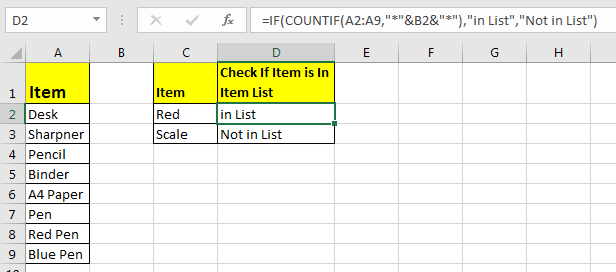
For this example, we have below sample data. We need a check-in the cell D2, if the given item in C2 exists in range A2:A9 or say item list. If it’s there then, print TRUE else FALSE.
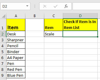
Write this formula in cell D2:
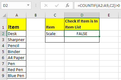
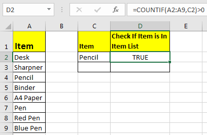
Since C2 contains “scale” and it’s not in the item list, it shows FALSE. Exactly as we wanted. Now if you replace “scale” with “Pencil” in the formula above, it’ll show TRUE.
Now, this TRUE and FALSE looks very back and white. How about customizing the output. I mean, how about we show, “found” or “not found” when value is in list and when it is not respectively.
Since this test gives us TRUE and FALSE, we can use it with IF function of excel.
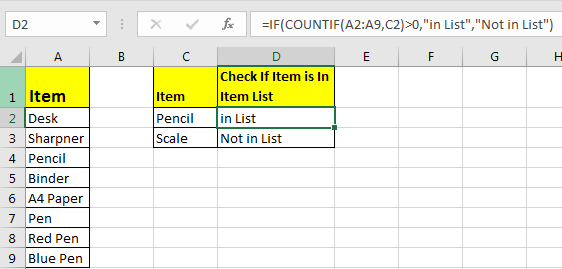
Write this formula:
=IF(COUNTIF(A2:A9,C2)>0,»in List»,»Not in List»)
You will have this as your output.
What If you remove “>0” from this if formula?
=IF(COUNTIF(A2:A9,C2),»in List»,»Not in List»)
It will work fine. You will have same result as above. Why? Because IF function in excel treats any value greater than 0 as TRUE.
How to check if a value is in Range with Wild Card Operators
Sometimes you would want to know if there is any match of your item in the list or not. I mean when you don’t want an exact match but any match.
For example, if in the above-given list, you want to check if there is anything with “red”. To do so, write this formula.
=IF(COUNTIF(A2:A9,»*red*»),»in List»,»Not in List»)
This will return a TRUE since we have “red pen” in our list. If you replace red with pink it will return FALSE. Try it.
Now here I have hardcoded the value in list but if your value is in a cell, say in our favourite cell B2 then write this formula.
IF(COUNTIF(A2:A9,»*»&B2&»*»),»in List»,»Not in List»)
There’s one more way to do the same. We can use the MATCH function in excel to check if the column contains a value. Let’s see how.
Find if a Value is in a List Using MATCH Function
So as we all know that MATCH function in excel returns the index of a value if found, else returns #N/A error. So we can use the ISNUMBER to check if the function returns a number.
If it returns a number ISNUMBER will show TRUE, which means it’s found else FALSE, and you know what that means.
Write this formula in cell C2:
=ISNUMBER(MATCH(C2,A2:A9,0))
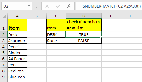
The MATCH function looks for an exact match of value in cell C2 in range A2:A9. Since DESK is on the list, it shows a TRUE value and FALSE for SCALE.
So yeah, these are the ways, using which you can find if a value is in the list or not and then take action on them as you like using IF function. I explained how to find value in a range in the best way possible. Let me know if you have any thoughts. The comments section is all yours.
Related Articles:
How to Check If Cell Contains Specific Text in Excel
How to Check A list of Texts In String in Excel
How to take the Average Difference between lists in Excel
How to Get Every Nth Value From A list in Excel
Popular Articles:
50 Excel Shortcuts to Increase Your Productivity
How to use the VLOOKUP Function in Excel
How to use the COUNTIF function in Excel
How to use the SUMIF Function in Excel
In this example, the goal is to use a formula to check if a specific value exists in a range. The easiest way to do this is to use the COUNTIF function to count occurences of a value in a range, then use the count to create a final result.
COUNTIF function
The COUNTIF function counts cells that meet supplied criteria. The generic syntax looks like this:
=COUNTIF(range,criteria)Range is the range of cells to test, and criteria is a condition that should be tested. COUNTIF returns the number of cells in range that meet the condition defined by criteria. If no cells meet criteria, COUNTIF returns zero. In the example shown, we can use COUNTIF to count the values we are looking for like this
COUNTIF(data,E5)Once the named range data (B5:B16) and cell E5 have been evaluated, we have:
=COUNTIF(data,E5)
=COUNTIF(B5:B16,"Blue")
=1
COUNTIF returns 1 because «Blue» occurs in the range B5:B16 once. Next, we use the greater than operator (>) to run a simple test to force a TRUE or FALSE result:
=COUNTIF(data,B5)>0 // returns TRUE or FALSEBy itself, the formula above will return TRUE or FALSE. The last part of the problem is to return a «Yes» or «No» result. To handle this, we nest the formula above into the IF function like this:
=IF(COUNTIF(data,E5)>0,"Yes","No")This is the formula shown in the worksheet above. As the formula is copied down, COUNTIF returns a count of the value in column E. If the count is greater than zero, the IF function returns «Yes». If the count is zero, IF returns «No».
Slightly abbreviated
It is possible to shorten this formula slightly and get the same result like this:
=IF(COUNTIF(data,E5),"Yes","No")Here, we have remove the «>0» test. Instead, we simply return the count to IF as the logical_test. This works because Excel will treat any non-zero number as TRUE when the number is evaluated as a Boolean.
Testing for a partial match
To test a range to see if it contains a substring (a partial match), you can add a wildcard to the formula. For example, if you have a value to look for in cell C1, and you want to check the range A1:A100 for partial matches, you can configure COUNTIF to look for the value in C1 anywhere in a cell by concatenating asterisks on both sides:
=COUNTIF(A1:A100,"*"&C1&"*")>0
The asterisk (*) is a wildcard for one or more characters. By concatenating asterisks before and after the value in C1, the formula will count the text in C1 anywhere it appears in each cell of the range. To return «Yes» or «No», nest the formula inside the IF function as above.
An alternative formula using MATCH
As an alternative, you can use a formula that uses the MATCH function with the ISNUMBER function instead of COUNTIF:
=ISNUMBER(MATCH(value,range,0))
The MATCH function returns the position of a match (as a number) if found, and #N/A if not found. By wrapping MATCH inside ISNUMBER, the final result will be TRUE when MATCH finds a match and FALSE when MATCH returns #N/A.