
Overview of formulas in Excel
Get started on how to create formulas and use built-in functions to perform calculations and solve problems.

Important: The calculated results of formulas and some Excel worksheet functions may differ slightly between a Windows PC using x86 or x86-64 architecture and a Windows RT PC using ARM architecture. Learn more about the differences.
Important: In this article we discuss XLOOKUP and VLOOKUP, which are similar. Try using the new XLOOKUP function, an improved version of VLOOKUP that works in any direction and returns exact matches by default, making it easier and more convenient to use than its predecessor.
Create a formula that refers to values in other cells
-
Select a cell.
-
Type the equal sign =.
Note: Formulas in Excel always begin with the equal sign.
-
Select a cell or type its address in the selected cell.

-
Enter an operator. For example, – for subtraction.
-
Select the next cell, or type its address in the selected cell.
-
Press Enter. The result of the calculation appears in the cell with the formula.


See a formula
-
When a formula is entered into a cell, it also appears in the Formula bar.
-
To see a formula, select a cell, and it will appear in the formula bar.


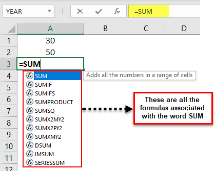
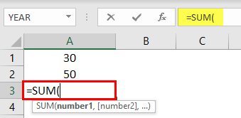
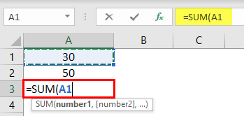
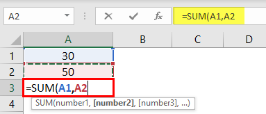
Enter a formula that contains a built-in function
-
Select an empty cell.
-
Type an equal sign = and then type a function. For example, =SUM for getting the total sales.
-
Type an opening parenthesis (.
-
Select the range of cells, and then type a closing parenthesis).
-
Press Enter to get the result.

Download our Formulas tutorial workbook
We’ve put together a Get started with Formulas workbook that you can download. If you’re new to Excel, or even if you have some experience with it, you can walk through Excel’s most common formulas in this tour. With real-world examples and helpful visuals, you’ll be able to Sum, Count, Average, and Vlookup like a pro.
Formulas in-depth
You can browse through the individual sections below to learn more about specific formula elements.
A formula can also contain any or all of the following: functions, references, operators, and constants.
Parts of a formula

1. Functions: The PI() function returns the value of pi: 3.142…
2. References: A2 returns the value in cell A2.
3. Constants: Numbers or text values entered directly into a formula, such as 2.
4. Operators: The ^ (caret) operator raises a number to a power, and the * (asterisk) operator multiplies numbers.
A constant is a value that is not calculated; it always stays the same. For example, the date 10/9/2008, the number 210, and the text «Quarterly Earnings» are all constants. An expression or a value resulting from an expression is not a constant. If you use constants in a formula instead of references to cells (for example, =30+70+110), the result changes only if you modify the formula. In general, it’s best to place constants in individual cells where they can be easily changed if needed, then reference those cells in formulas.
A reference identifies a cell or a range of cells on a worksheet, and tells Excel where to look for the values or data you want to use in a formula. You can use references to use data contained in different parts of a worksheet in one formula or use the value from one cell in several formulas. You can also refer to cells on other sheets in the same workbook, and to other workbooks. References to cells in other workbooks are called links or external references.
-
The A1 reference style
By default, Excel uses the A1 reference style, which refers to columns with letters (A through XFD, for a total of 16,384 columns) and refers to rows with numbers (1 through 1,048,576). These letters and numbers are called row and column headings. To refer to a cell, enter the column letter followed by the row number. For example, B2 refers to the cell at the intersection of column B and row 2.
To refer to
Use
The cell in column A and row 10
A10
The range of cells in column A and rows 10 through 20
A10:A20
The range of cells in row 15 and columns B through E
B15:E15
All cells in row 5
5:5
All cells in rows 5 through 10
5:10
All cells in column H
H:H
All cells in columns H through J
H:J
The range of cells in columns A through E and rows 10 through 20
A10:E20
-
Making a reference to a cell or a range of cells on another worksheet in the same workbook
In the following example, the AVERAGE function calculates the average value for the range B1:B10 on the worksheet named Marketing in the same workbook.
1. Refers to the worksheet named Marketing
2. Refers to the range of cells from B1 to B10
3. The exclamation point (!) Separates the worksheet reference from the cell range reference
Note: If the referenced worksheet has spaces or numbers in it, then you need to add apostrophes (‘) before and after the worksheet name, like =’123′!A1 or =’January Revenue’!A1.
-
The difference between absolute, relative and mixed references
-
Relative references A relative cell reference in a formula, such as A1, is based on the relative position of the cell that contains the formula and the cell the reference refers to. If the position of the cell that contains the formula changes, the reference is changed. If you copy or fill the formula across rows or down columns, the reference automatically adjusts. By default, new formulas use relative references. For example, if you copy or fill a relative reference in cell B2 to cell B3, it automatically adjusts from =A1 to =A2.
Copied formula with relative reference
-
Absolute references An absolute cell reference in a formula, such as $A$1, always refer to a cell in a specific location. If the position of the cell that contains the formula changes, the absolute reference remains the same. If you copy or fill the formula across rows or down columns, the absolute reference does not adjust. By default, new formulas use relative references, so you may need to switch them to absolute references. For example, if you copy or fill an absolute reference in cell B2 to cell B3, it stays the same in both cells: =$A$1.
Copied formula with absolute reference
-
Mixed references A mixed reference has either an absolute column and relative row, or absolute row and relative column. An absolute column reference takes the form $A1, $B1, and so on. An absolute row reference takes the form A$1, B$1, and so on. If the position of the cell that contains the formula changes, the relative reference is changed, and the absolute reference does not change. If you copy or fill the formula across rows or down columns, the relative reference automatically adjusts, and the absolute reference does not adjust. For example, if you copy or fill a mixed reference from cell A2 to B3, it adjusts from =A$1 to =B$1.
Copied formula with mixed reference
-
-
The 3-D reference style
Conveniently referencing multiple worksheets If you want to analyze data in the same cell or range of cells on multiple worksheets within a workbook, use a 3-D reference. A 3-D reference includes the cell or range reference, preceded by a range of worksheet names. Excel uses any worksheets stored between the starting and ending names of the reference. For example, =SUM(Sheet2:Sheet13!B5) adds all the values contained in cell B5 on all the worksheets between and including Sheet 2 and Sheet 13.
-
You can use 3-D references to refer to cells on other sheets, to define names, and to create formulas by using the following functions: SUM, AVERAGE, AVERAGEA, COUNT, COUNTA, MAX, MAXA, MIN, MINA, PRODUCT, STDEV.P, STDEV.S, STDEVA, STDEVPA, VAR.P, VAR.S, VARA, and VARPA.
-
3-D references cannot be used in array formulas.
-
3-D references cannot be used with the intersection operator (a single space) or in formulas that use implicit intersection.
What occurs when you move, copy, insert, or delete worksheets The following examples explain what happens when you move, copy, insert, or delete worksheets that are included in a 3-D reference. The examples use the formula =SUM(Sheet2:Sheet6!A2:A5) to add cells A2 through A5 on worksheets 2 through 6.
-
Insert or copy If you insert or copy sheets between Sheet2 and Sheet6 (the endpoints in this example), Excel includes all values in cells A2 through A5 from the added sheets in the calculations.
-
Delete If you delete sheets between Sheet2 and Sheet6, Excel removes their values from the calculation.
-
Move If you move sheets from between Sheet2 and Sheet6 to a location outside the referenced sheet range, Excel removes their values from the calculation.
-
Move an endpoint If you move Sheet2 or Sheet6 to another location in the same workbook, Excel adjusts the calculation to accommodate the new range of sheets between them.
-
Delete an endpoint If you delete Sheet2 or Sheet6, Excel adjusts the calculation to accommodate the range of sheets between them.
-
-
The R1C1 reference style
You can also use a reference style where both the rows and the columns on the worksheet are numbered. The R1C1 reference style is useful for computing row and column positions in macros. In the R1C1 style, Excel indicates the location of a cell with an «R» followed by a row number and a «C» followed by a column number.
Reference
Meaning
R[-2]C
A relative reference to the cell two rows up and in the same column
R[2]C[2]
A relative reference to the cell two rows down and two columns to the right
R2C2
An absolute reference to the cell in the second row and in the second column
R[-1]
A relative reference to the entire row above the active cell
R
An absolute reference to the current row
When you record a macro, Excel records some commands by using the R1C1 reference style. For example, if you record a command, such as clicking the AutoSum button to insert a formula that adds a range of cells, Excel records the formula by using R1C1 style, not A1 style, references.
You can turn the R1C1 reference style on or off by setting or clearing the R1C1 reference style check box under the Working with formulas section in the Formulas category of the Options dialog box. To display this dialog box, click the File tab.
Top of Page


Need more help?
You can always ask an expert in the Excel Tech Community or get support in the Answers community.
See Also
Switch between relative, absolute and mixed references for functions
Using calculation operators in Excel formulas
The order in which Excel performs operations in formulas
Using functions and nested functions in Excel formulas
Define and use names in formulas
Guidelines and examples of array formulas
Delete or remove a formula
How to avoid broken formulas
Find and correct errors in formulas
Excel keyboard shortcuts and function keys
Excel functions (by category)
Need more help?
Want more options?
Explore subscription benefits, browse training courses, learn how to secure your device, and more.
Communities help you ask and answer questions, give feedback, and hear from experts with rich knowledge.
Excel is full of formulas. Those who master those formulas are pros of Excel. However, at the start of learning Excel, everyone is curious to know how to apply or create formulas in Excel. If you are one of them who is willing to learn how to create formulas in Excel, then this article is best suited for you. This article will have a complete guide from zero to intermediate level formula application in Excel.
Let us create a simple calculator-type formula for adding up numbers to start with Excel formulas.
You can download this Create a Formula Excel Template here – Create a Formula Excel Template
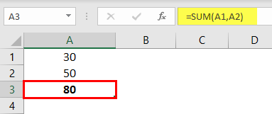
Look at the below data of numbers.
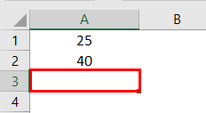
In cell A1, we have 25. The A2 cell has 40, the number.
In cell A3, we need the summation of these two numbers.
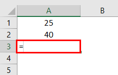
In Excel, to start the formula, always put the equal sign first.
Now, insert 25 + 40 as the equation.
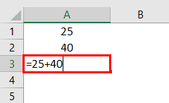
It is very similar to what we do in the calculator.
Press the “Enter” key to get the total of these numbers.

So, 25 + 40 is 65, the same we got in cell A3.
Table of contents
- How to Create a Formula in Excel?
- #1 Create Formula Flexible with Cell References
- #2 Use SUM Function to Add Up Numbers
- #3 Create Formula References to Other Cells Excel
- Recommended Articles
#1 Create Formula Flexible with Cell References
Let us start.
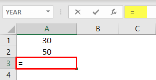
- From the above example, we will change the number from 25 to 30 and 40 to 50.

Even though we have changed numbers in cells A1 and A2, our formula only shows the old result of 65. It is a problem with direct numbers passing to the formula. It does not make the formula flexible enough to update the new result.
- We can give cell reference as the formula reference to overcoming this issue. For example, open the equal sign in cell A3.

- Then, select cell A1.

- Insert plus (+) sign and select cell A2.

- Press the “Enter” key to get the result.


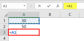
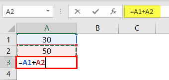
As we can see in the formula bar, it is not showing the result. Rather, it shows the formula itself, and cell A3 shows the result of the formula.
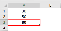
Now, we can change the numbers in A1 and A2 cells to see the immediate impact of the formula.
#2 Use SUM Function to Add Up Numbers
To get used to the formulas in Excel, let us start with the simple SUM function. All the formulas should begin with “+” or “=.” So, open the equal sign in cell A3.
Start typing the SUM to see the intellisense list of Excel functionsExcel functions help the users to save time and maintain extensive worksheets. There are 100+ excel functions categorized as financial, logical, text, date and time, Lookup & Reference, Math, Statistical and Information functions.read more.
Press the “Tab” key once the SUM formula is selected to open the SUM function in excel.The SUM function in excel adds the numerical values in a range of cells. Being categorized under the Math and Trigonometry function, it is entered by typing “=SUM” followed by the values to be summed. The values supplied to the function can be numbers, cell references or ranges.read more
The first argument of the SUM function is Number 1, whichis the first number we need to add. In this example, cell A1. So, we must select cell A1.
The next argument is Number 2, the second number or item we need to add, A2 cell.
Now, we must close the bracket and press the “Enter” key to see the result of the SUM function.
Like this, we can create simple formulas in Excel to do the calculations.
#3 Create Formula References to Other Cells Excel
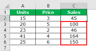
We have seen the basics of creating a formula in Excel. Similarly, we can apply one formula to other related cells as well. For example, look at the below data.
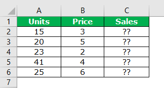
In column A we have “Units.” In column B, we have the “Price Per Unit.”
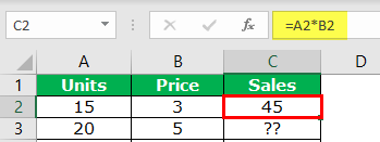
In the column, C needs to arrive at “Sales Amount.” For arriving at the sales amount, the formula is Units * Price.
- So, we must open an equal sign in cell C2.
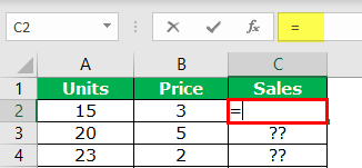
- Select cell A2 (units).
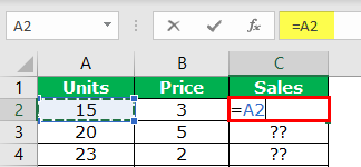
- Enter multiple sign (*) and select the B2 cell (price).
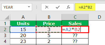
- Press the “Enter” key to get the sales amount.
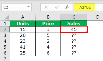
Now, we have applied the formula in cell C2. How about the remaining cells?
Can you enter the same formula for the remaining cells individually?
If you think that way, you will be delighted to hear that the “formula is to be applied to a single cell, then we can copy-paste to other cells.”
Now first, look at the formula we have applied.
The formula says A2 * B2.
So, when we copy and paste the formula below, cell A2 becomes A3, and B2 becomes B3.
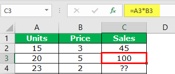
Similarly, row numbers keep changing as we move down, and column letters will also change if we move either left or right.
- Copy and paste the formula to other cells to result in all the cells.
Like this, we can create a simple formula in Excel to start your learning.
Recommended Articles
This article has been a guide to creating a formula in Excel. Here, we learn to create a simple Excel formula and practical examples, and a downloadable template. You may learn more about Excel from the following articles: –
- Write Formula in Excel
- PI in Excel
- Excel Formula Not Working
- List of Basic Excel Formulas
[icon name=”calendar” class=”” unprefixed_class=””] DATE & TIME
DateDif
EndOfMonth
Time
Weekday
Weeknum
Workday
Year
[icon name=”lightbulb-o” class=”” unprefixed_class=””] LOGICAL
And
If
If, And
Iferror
[icon name=”arrow-circle-up” class=”” unprefixed_class=””] LOOKUP
Array, Lookup
Hlookup
Iferror, Vlookup
Index
Index, Match
Indirect
Match
Multiple Criteria, Vlookup
Offset
Pivot Table, GetPivotData
Sum, Lookup
Vlookup
Xlookup
[icon name=”calculator” class=”” unprefixed_class=””] MATH
Average
Count
CountA
CountBlank
CountIf
CountIfs
Mathematical Formulas
Mod
Percentage
Rand
Randbetween
Round
Subtotal
Sumifs
Sumproduct
[icon name=”delicious” class=”” unprefixed_class=””] OTHER
3D
Array
Chart
Convert, Values
Evaluate
Find & Select
FV
Reference
Show, Hide
Transpose
Type
Value
[icon name=”wpforms” class=”” unprefixed_class=””] TEXT
Between
Clean
Concatenate
Data Cleansing, Trim
Extract, Find, Left
Left
Len, Length
Proper
Remove
Remove, Substitute
Replace
Replace, Cleanup
Right
Substitute
Substitute, Trim
Text
Upper
[icon name=”wpforms” class=”” unprefixed_class=””] OFFICE 365
Filter
Sort
Sortby
Unique
Click on any Excel formula & function link below and it will take you to the advanced Excel formulas with examples in Excel sheet free download for you to practice!
The array of Excel functions allows you to solve complex tasks in automatically at the same time. We cannot complete the same tasks through the usual functions.
In fact, this is a group of functions that simultaneously process a group of data and immediately produce a result. Let’s consider in detail work with arrays of functions in Excel.
Types of Excel functions
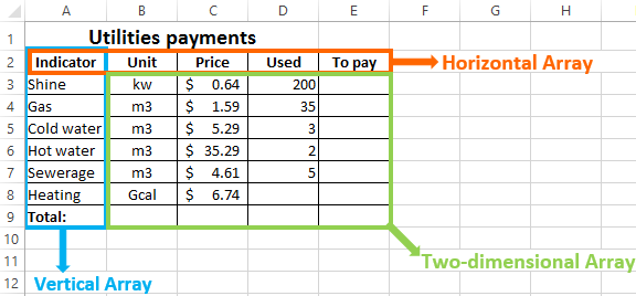
Array is a data grouped together. In this case, the group is an array of functions in Excel. Any table that we compose and fill in Excel can be called an array. Example:
Depending on the location of the elements, the arrays are distinguished:
- One-dimensional (data is in ONE line or in ONE column);
- Two-dimensional (SEVERAL lines and columns, matrix).
One-dimensional arrays are:
- Horizontal (data in a row);
- Vertical (data in a column).
Note. Two-dimensional Excel arrays can take several sheets at once (these are hundreds and thousands of data).
Array formula allows you to process data from this array. It can return one value or result in an array (set) of values.
With the help of array formulas it is real to:
- Count the number of characters in a certain range;
- Summarize only those numbers that correspond to the given condition;
- Summarize all n values in a certain range.
When we use array formulas, Excel takes into account the range of values not as individual cells, but as a single data block.
Array formulas syntax
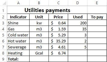
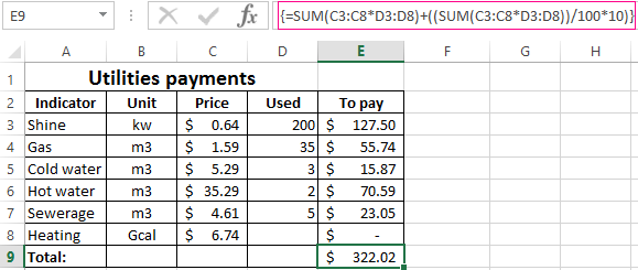
We use the formula of an array with a range of cells and with a separate cell. In the first case, we find the subtotals for the «To pay» «» column. In the second — the total amount of utility payments.
- We select the range E3: E8.
- Enter the following formula in the formula row: = C3: C8 * D3: D8.
- Press the keys simultaneously: Ctrl + Shift + Enter. The subtotals are calculated:
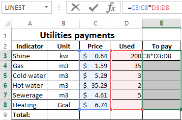
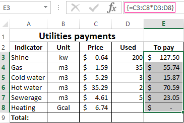
The formula after pressing Ctrl + Shift + Enter was in curly brackets. It was automatically inserted into each cell of the selected range.
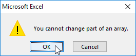
If you try to change the data in any cell in the «To pay» column, nothing happens. The formula in the array protects range values from changes. A corresponding entry appears on the screen:
Consider other examples of using the functions of an Excel array — calculate the total amount of utility payments using a single formula.
- Select the cell E9 (opposite the «Total»).
- We introduce a formula of the form:
- Press the key combination: Ctrl + Shift + Enter. Result:
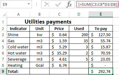
The formula of the array in this case replaced two simple formulas. This is a shortened version, which contains all the necessary information for solving a complex problem.
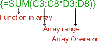
Arguments for a function are one-dimensional arrays. The formula looks at each of them individually, performs user-defined operations, and generates a single result.
Consider the syntax:
Working functions with Excel array
Let’s guess that it is planned to increase utility payments in 10% the next month. If we introduce the usual formula for the total is =SUM((C3:C8*D3:D8)+10%), then we are unlikely to get the expected result. We need each argument to increase in 10%. For the program to understand this, we use the function as an array.
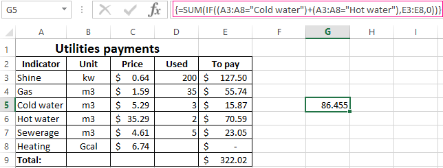
- Let’s have a look how the «И» «AND» operator works in the array function. We need to find out how much we pay for the water, hot and cold. Function:
The total is 86.46$.
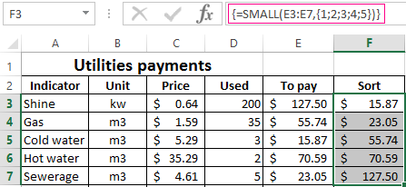
- The Sort functions in the array formula. Sort the amounts to be paid in ascending order. For the sorted data list, create a range. Let’s select it (F3:F7). In the formula bar, we enter
Press Ctrl + Shift + Enter.
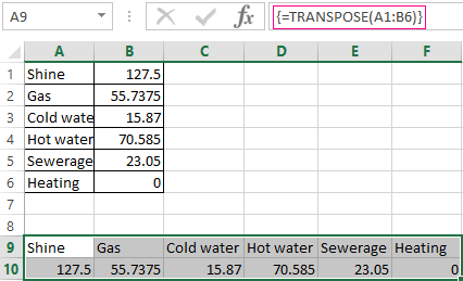
- The transported matrix. There is a special Excel function for working with two-dimensional arrays. The «ТРАНСП» function returns several values at once. It converts a horizontal matrix to a vertical matrix and vice versa. Select the range of cells where the number of rows equals to the number of columns in the table with the original data. And the number of columns equals to the number of rows in the source array. Select range A9:F10. We introduce the formula:
Press Ctrl + Shift + Enter. This results in an «inverted» data set.
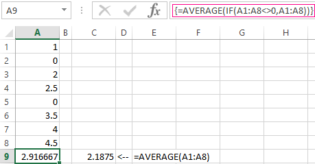
- Search for the average without taking into account zeros. If we use the standard «AVERAGE» function, we get «0» as a result. And it will be correct. Therefore, we insert an additional condition into the formula:
We get:
A common mistake when working with arrays of functions is NOT to press the code combination «Ctrl + Shift + Enter» (never forget this key combination). This is the most important thing to remember when processing large amounts of information. Correctly entered function performs the most complicated tasks.
Download array formula examples
Time-saving ways to insert formulas into Excel
Basic Excel Formulas Guide
Mastering the basic Excel formulas is critical for beginners to become highly proficient in financial analysis. Microsoft Excel is considered the industry standard piece of software in data analysis. Microsoft’s spreadsheet program also happens to be one of the most preferred software by investment bankers and financial analysts in data processing, financial modeling, and presentation.
This guide will provide an overview and list of some basic Excel functions.
Once you’ve mastered this list, move on to CFI’s advanced Excel formulas guide!
Basic Terms in Excel
There are two basic ways to perform calculations in Excel: Formulas and Functions.
1. Formulas
In Excel, a formula is an expression that operates on values in a range of cells or a cell. For example, =A1+A2+A3, which finds the sum of the range of values from cell A1 to cell A3.
2. Functions
Functions are predefined formulas in Excel. They eliminate laborious manual entry of formulas while giving them human-friendly names. For example: =SUM(A1:A3). The function sums all the values from A1 to A3.
Key Highlights
- Excel is still the industry benchmark for financial analysis and modeling across almost all corporate finance functions. This course is designed to highlight some of the most important basic Excel formulas.
- Mastering these will help a learner build confidence in Excel and move on to more difficult functions and formulas.
- There are also several different ways to enter a function in Excel, as shown below.
Five Time-saving Ways to Insert Data into Excel
When analyzing data, there are five common ways of inserting basic Excel formulas. Each strategy comes with its own advantages. Therefore, before diving further into the main formulas, we’ll clarify those methods, so you can create your preferred workflow earlier on.
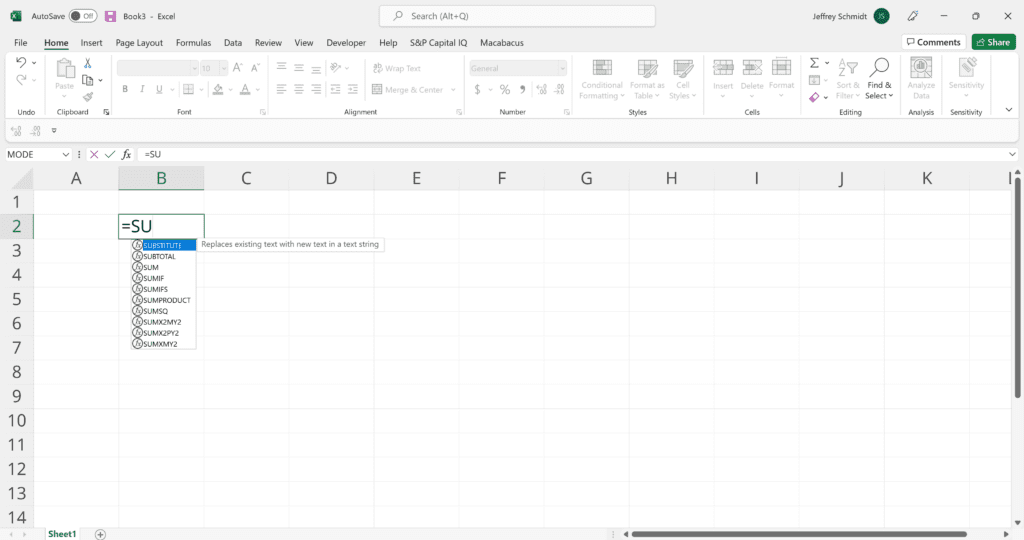
1. Simple insertion: Typing a formula inside the cell
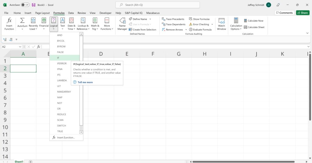
Typing a formula in a cell or the formula bar is the most straightforward method of inserting basic Excel formulas. The process usually starts by typing an equal sign, followed by the name of an Excel function.
Excel is quite intelligent in that when you start typing the name of the function, a pop-up function hint will show (see below). It’s from this list you’ll select your preference. However, don’t press the Enter key after making your selection. Instead, press the Tab key and Excel will automatically fill in the function name.
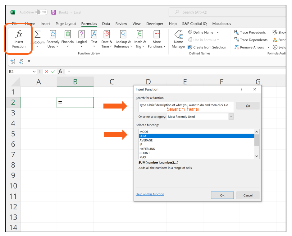
2. Using Insert Function Option from Formulas Tab
If you want full control of your function’s insertion, using the Excel Insert Function dialogue box is all you ever need. To achieve this, go to the Formulas tab and select the first menu labeled Insert Function. The dialogue box will contain all the functions you need to complete your financial analysis.
3. Selecting a Formula from One of the Groups in Formula Tab
This option is for those who want to delve into their favorite functions quickly. To find this menu, navigate to the Formulas tab and select your preferred group. Click to show a sub-menu filled with a list of functions.
From there, you can select your preference. However, if you find your preferred group is not on the tab, click on the More Functions option – it’s probably just hidden there.
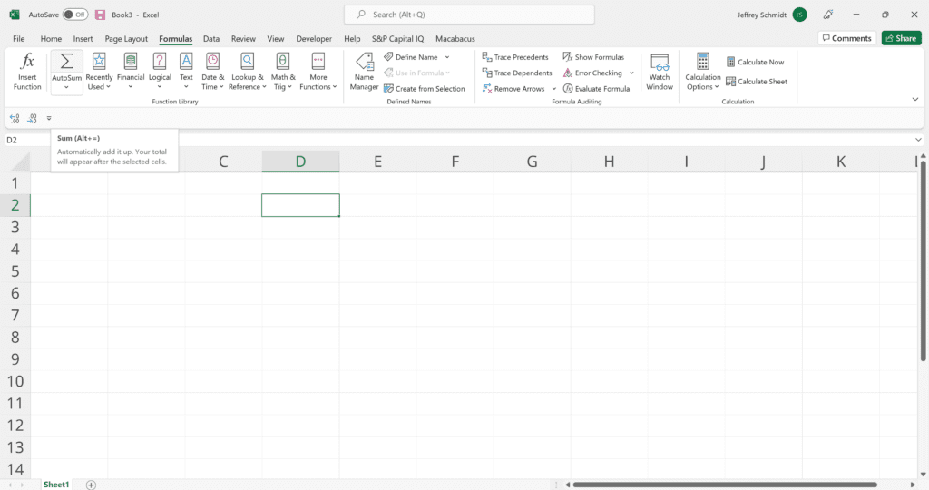
4. Using AutoSum Option
For quick and everyday tasks, the AutoSum function is your go-to option. Navigate to the Formulas tab and click the AutoSum option. Then click the caret to show other hidden formulas. This option is also available in the Home tab.
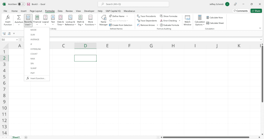
5. Quick Insert: Use Recently Used Tabs
If you find re-typing your most recent formula a monotonous task, then use the Recently Used selection. It’s on the Formulas tab, a third menu option just next to AutoSum.
Free Excel Formulas YouTube Tutorial
Watch CFI’s FREE video tutorial to quickly learn the most important Excel formulas. By watching the video demonstration you’ll quickly learn the most important formulas and functions.
Seven Basic Excel Formulas For Your Workflow
Since you’re now able to insert your preferred formulas and function correctly, let’s check some fundamental Excel functions to get you started.
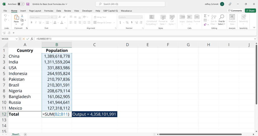
1. SUM
The SUM function is the first must-know formula in Excel. It usually aggregates values from a selection of columns or rows from your selected range.
=SUM(number1, [number2], …)
Example:
=SUM(B2:G2) – A simple selection that sums the values of a row.
=SUM(A2:A8) – A simple selection that sums the values of a column.
=SUM(A2:A7, A9, A12:A15) – A sophisticated collection that sums values from range A2 to A7, skips A8, adds A9, jumps A10 and A11, then finally adds from A12 to A15.
=SUM(A2:A8)/20 – Shows you can also turn your function into a formula.
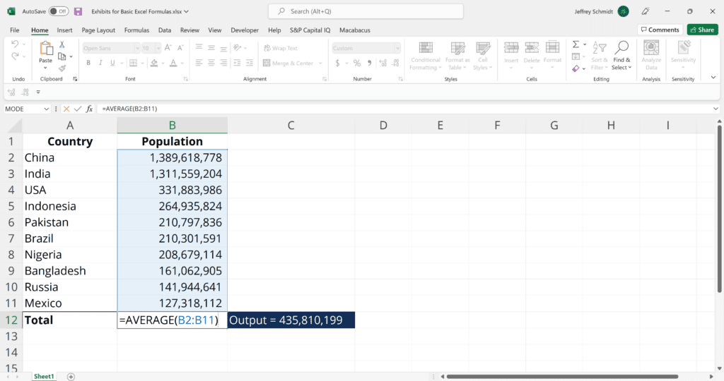
2. AVERAGE
The AVERAGE function should remind you of simple averages of data, such as the average number of shareholders in a given shareholding pool.
=AVERAGE(number1, [number2], …)
Example:
=AVERAGE(B2:B11) – Shows a simple average, also similar to (SUM(B2:B11)/10)
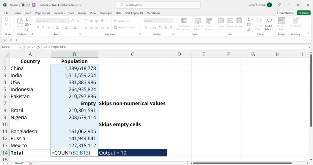
3. COUNT
The COUNT function counts all cells in a given range that contain only numeric values.
=COUNT(value1, [value2], …)
Example:
COUNT(A:A) – Counts all values that are numerical in A column. However, you must adjust the range inside the formula to count rows.
COUNT(A1:C1) – Now it can count rows.
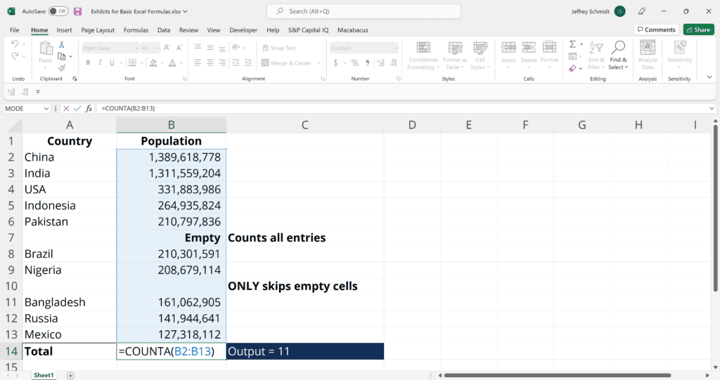
4. COUNTA
Like the COUNT function, COUNTA counts all cells in a given rage. However, it counts all cells regardless of type. That is, unlike COUNT that only counts numerics, it also counts dates, times, strings, logical values, errors, empty string, or text.
=COUNTA(value1, [value2], …)
Example:
COUNTA(C2:C13) – Counts rows 2 to 13 in column C regardless of type. However, like COUNT, you can’t use the same formula to count rows. You must make an adjustment to the selection inside the brackets – for example, COUNTA(C2:H2) will count columns C to H
5. IF
The IF function is often used when you want to sort your data according to a given logic. The best part of the IF formula is that you can embed formulas and functions in it.
=IF(logical_test, [value_if_true], [value_if_false])
Example:
=IF(C2<D3,“TRUE”,”FALSE”) – Checks if the value at C3 is less than the value at D3. If the logic is true, let the cell value be TRUE, otherwise, FALSE
=IF(SUM(C1:C10) > SUM(D1:D10), SUM(C1:C10), SUM(D1:D10)) – An example of a complex IF statement. First, it sums C1 to C10 and D1 to D10, then it compares the sum. If the sum of C1 to C10 is greater than the sum of D1 to D10, then it makes the value of a cell equal to the sum of C1 to C10.

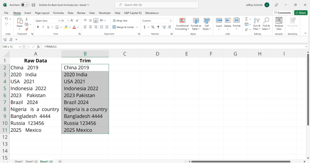
6. TRIM
The TRIM function makes sure your functions do not return errors due to extra spaces in your data. It ensures that all empty spaces are eliminated. Unlike other functions that can operate on a range of cells, TRIM only operates on a single cell. Therefore, it comes with the downside of adding duplicated data to your spreadsheet.
=TRIM(text)
Example:
TRIM(A2) – Removes empty spaces in the value in cell A2.
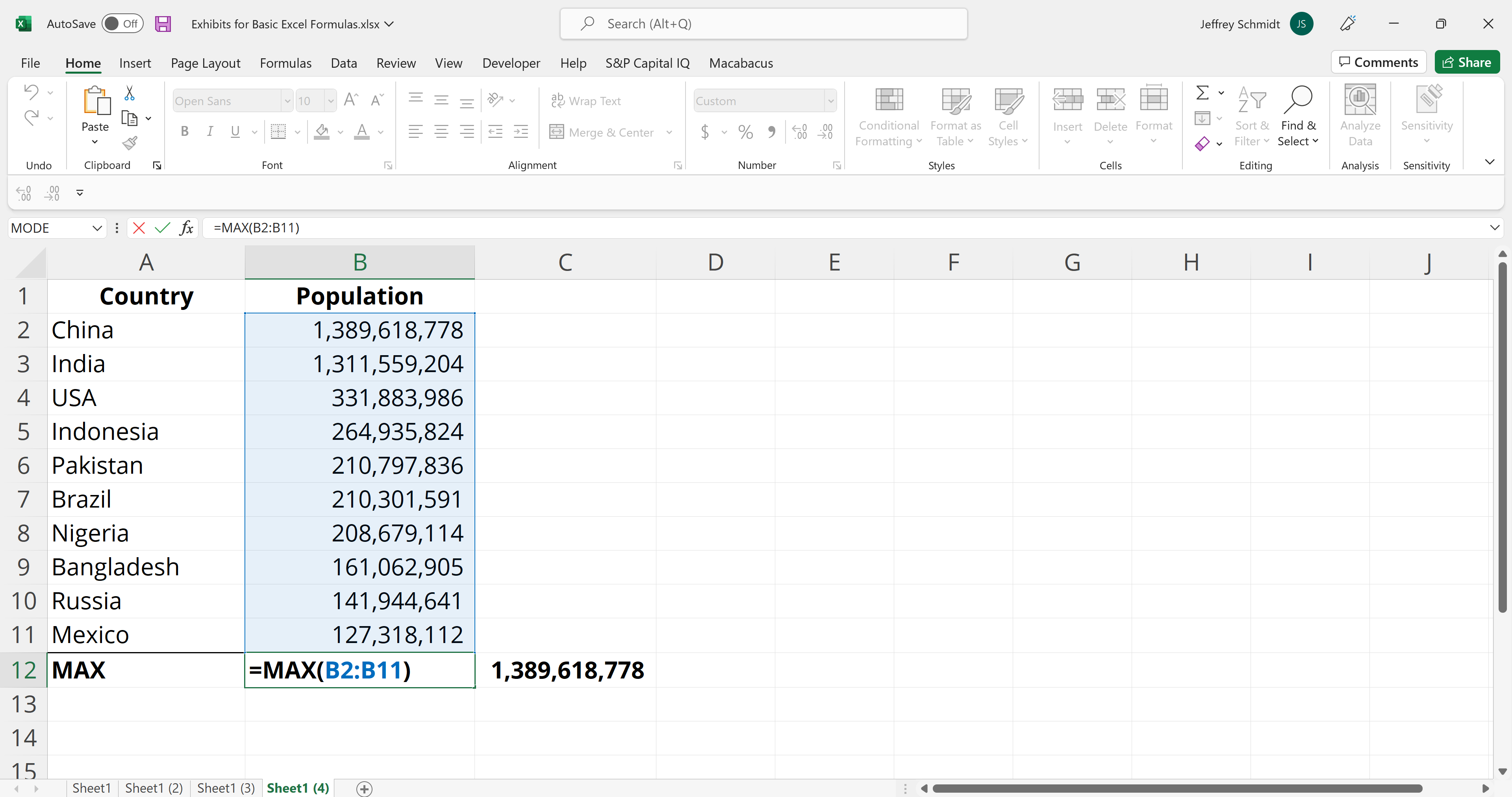
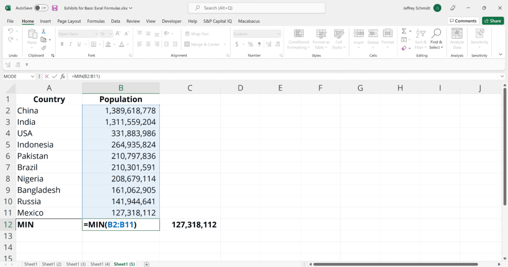
7. MAX & MIN
The MAX and MIN functions help in finding the maximum number and the minimum number in a range of values.
=MIN(number1, [number2], …)
Example:
=MIN(B2:C11) – Finds the minimum number between column B from B2 and column C from C2 to row 11 in both columns B and C.
=MAX(number1, [number2], …)
Example:
=MAX(B2:C11) – Similarly, it finds the maximum number between column B from B2 and column C from C2 to row 11 in both columns B and C.
More Resources
Thank you for reading CFI’s guide to basic Excel formulas. To continue your development as a world-class financial analyst, these additional CFI resources will be helpful:
- Advanced Excel Formulas
- Benefits of Excel Shortcuts
- Valuation Modeling in Excel
- See all Excel resources