
Watch video – Insert and Use Checkmark Symbol in Excel
Below is the written tutorial, in case you prefer reading over watching the video.
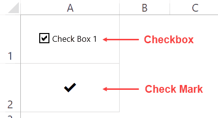
In Excel, there are two kinds of tick marks (✓) that you can insert – a check mark and a checkbox.
And no… these are not the same.
Let me explain.
Check Mark Vs Check Box
While a check mark and a checkbox may look somewhat similar, these two are very different in the way it can be inserted and used in Excel.
A check mark is a symbol that you can insert in a cell (just like any text that you type). This means that when you copy the cell, you also copy the check mark and when you delete the cell, you also delete the check mark. Just like regular text, you can format it by changing the color and font size.
A checkbox, on the other hand, is an object that sits above the worksheet. So when you place a checkbox above a cell, it’s not a part of the cell but is an object that is over it. This means that if you delete the cell, the checkbox may not get deleted. Also, you can select a checkbox and drag it anywhere in the worksheet (as it’s not bound to the cell).
You will find checkboxes being used in interactive reports and dashboards, while a checkmark is a symbol that you may want to include as a part of the report.
A check mark is a symbol in the cell and a checkbox (which is literally in a box) is an object that is placed above the cells.
In this article, I will only be covering check marks. If you want to learn more about checkbox, here is a detailed tutorial.
There are quite a few ways that you can use to insert a check mark symbol in Excel.
Click here to download the example file and follow along
Inserting Check Mark Symbol in Excel
In this article, I will show you all the methods I know.
The method you use would be dependent on how you want to use the check mark in your work (as you’ll see later in this tutorial).
Let’s get started!
Copy and Paste the Check Mark
Starting with the easiest one.
Since you’re already reading this article, you can copy the below check mark and paste it in Excel.
To do this, copy the check mark and go to the cell where you want to copy it. Now either double-click on the cell or press the F2 key. This will take you to the edit mode.
✔
Simply paste the check mark (Control + V).
Once you have the check mark in Excel, you can copy it and paste it as many times as you want.
This method is suited when you want to copy paste the check mark in a few places. Since this involves doing it manually, it’s not meant for huge reports where you have to insert check marks for hundreds or thousands of cells based on criteria. In such a case, it’s better to use a formula (as shown later in this tutorial).
Use the Keyboard Shortcuts
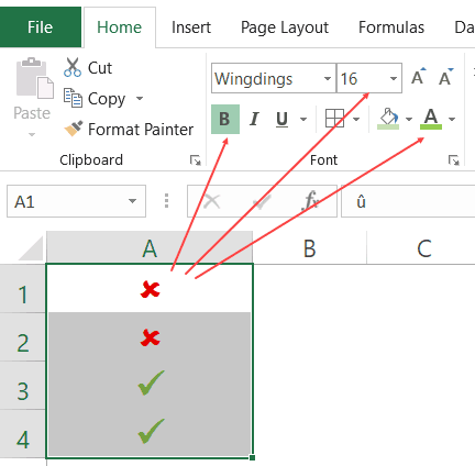
For using the keyboard shortcuts, you will have to change the font of the cells to Wingdings 2 (or Wingdings based on the keyboard shortcut you’re using).
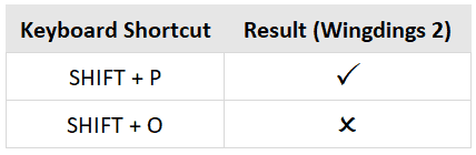
Below are the shortcuts for inserting a check mark or a cross symbol in cells. To use the below shortcuts, you need to change the font to Wingdings 2.
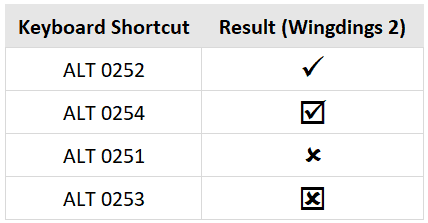
Below are some more keyboard shortcuts that you can use to insert check mark and cross symbols. To use the below shortcuts, you need to change the font to Wingdings (without the 2).
This method is best suited when you only want a check mark in the cell. Since this method requires you to change the font to Wingdings or Wingdings 2, it will not be useful if you want to have any other text or numbers in the same cell with the check mark or the cross mark.
Using the Symbols Dialog Box
Another way to insert a check mark symbol (or any symbol for that matter) in Excel is using the Symbol dialog box.
Here are the steps to insert the check mark (tick mark) using the Symbol dialog box:
- Select the cell in which you want the check mark symbol.
- Click the Insert tab in the ribbon.

- Click on the Symbol icon.

- In the Symbol dialog box that opens, select ‘Segoe UI Symbol’ as the font.

- Scroll down till you find the check mark symbol and the double click on it (or click on Insert).


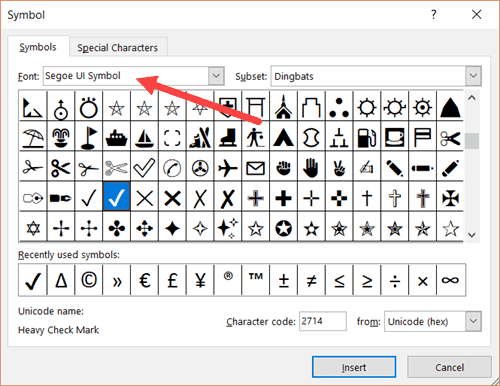
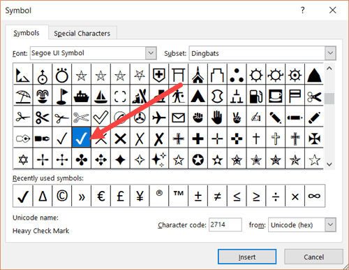
The above steps would insert one check mark in the selected cell.
If you want more, simply copy the already inserted one and use it.
Note that using ‘Segoe UI Symbol’ allows you to use the check mark in any regularly used font in Excel (such as Arial, Time Now, Calibri, or Verdana). The shape and size may adjust a little based on the font. This also means that you can have text/number along with the check mark in the same cell.
This method is a bit longer but doesn’t require you to know any shortcut or CHAR code. Once you have used it to insert the symbol, you can reuse that one by copy pasting it.
Using the CHAR Formula
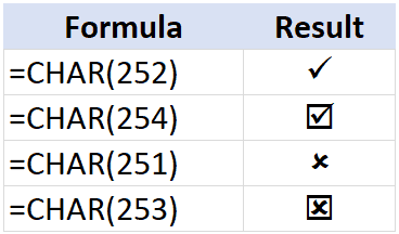
You can use the CHAR function to return a check mark (or a cross mark).
The below formula would return a check mark symbol in the cell.
=CHAR(252)
For this to work, you need to convert the font to Wingdings
Why?
Because when you use the CHAR(252) formula, it would give you the ANSI character (ü), and then when you change the font to Wingdings, it is converted to a check mark.
You can use similar CHAR formulas (with different code number) to get another format of the check mark or the cross mark.
The real benefit of using a formula is when you use it with other formulas and return the check mark or the cross mark as the result.
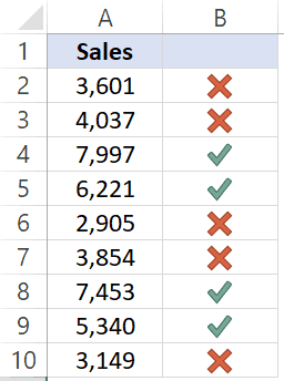
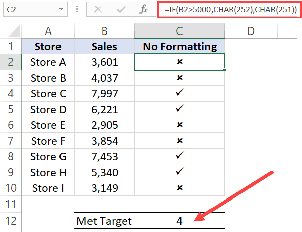
For example, suppose you have a dataset as shown below:
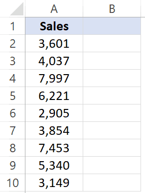
You can use the below IF formula to get a check mark if the sale value is more than 5000 and a cross mark if it’s less than 5000.
=IF(A2>5000,CHAR(252),CHAR(251))
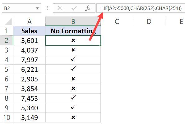
Remember, you need to convert the column font to Wingdings.
This helps you make your reports a little more visual. It also works well with printed reports.
If you want to remove the formula and only keep the values, copy the cell and paste it as value (right-click and choose the Paste Special and then click on Paste and Values icon).
This method is suited when you want the check mark insertion to be dependent on cell values. Since this uses a formula, you can use it even when you have hundreds or thousands of cells. Also, since you need to change the font of the cells to Wingdings, you can’t have anything else in the cells except the symbols.
Using Autocorrect
Excel has a feature where it can autocorrect misspelled words automatically.
For example, type the word ‘bcak’ in a cell in Excel and see what happens. It will automatically correct it to the word ‘back’.
This happens as there is already a pre-made list of expected misspelled words you’re likely to type and Excel automatically corrects it for you.
Here are the steps to use autocorrect to insert the delta symbol:
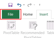
- Click on the File tab.

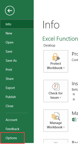
- Click on Options.

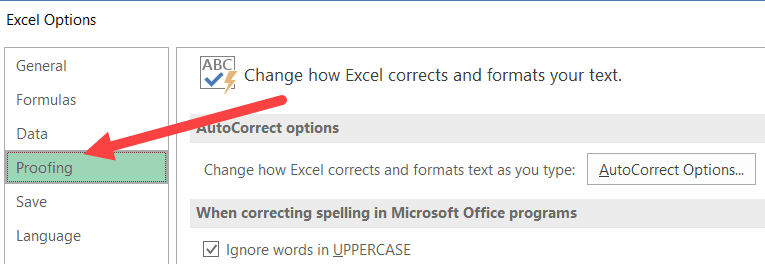
- In the Options dialogue box, select Proofing.

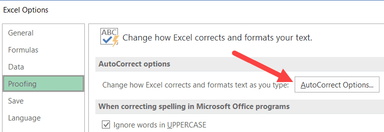
- Click on the ‘AutoCorrect Options’ button.
- In the Autocorrect dialogue box, enter the following:
- Replace: CMARK
- With: ✔ (you can copy and paste this)

- Click Add and then OK.

Now whenever you type the words CMARK in a cell in Excel, it will automatically change it to a check mark.
Here are a few things you need to know when using the Autocorrect method:
- This is case sensitive. So if you enter ‘cmark’, it will not get converted into the check mark symbol. You need to enter CMARK.
- This change also gets applied to all the other Microsoft applications (MS Word, PowerPoint, etc.). So be cautious and choose the keyword that you are highly unlikely to use in any other application.
- If there is any text/number before/after CMARK, it will not be converted to the check mark symbol. For example, ‘38%CMARK’ will not get converted, however, ‘38% CMARK’ will get converted to ‘38% ✔’
Related Tutorial: Excel Autocorrect
This method is suited when you want a ready reference for the check mark and you use it regularly in your work. So instead of remembering the shortcuts or using the symbols dialog box, you can quickly use the shortcode name that you have created for check mark (or any other symbol for that matter).
Click here to download the example file and follow along
Using Conditional Formatting to Insert Check Mark
You can use conditional formatting to insert a check mark or a cross mark based on the cell value.
For example, suppose you have the data set as shown below and you want to insert a check mark if the value is more than 5000 and a cross mark if it’s less than 5000.
Here are the steps to do this using conditional formatting:
- In cell B2, enter =A2, and then copy this formula for all cells. This will make sure that now you have the same value in the adjacent cell and if you change the value in column A, it’s automatically changed in column B.

- Select all the cells in column B (in which you want to insert the check mark).
- Click the Home tab.
- Click on Conditional Formatting.
- Click on New Rule.

- In the ‘New Formatting Rule’ dialog box, click on the ‘Format Style’ drop down and click on ‘Icon Sets’.

- In the ‘Icon Style’ drop-down, select the style with the check mark and cross mark.

- Check the ‘Show Icon only’ box. This will ensure that only the icons are visible and the numbers are hidden.
- In the Icon settings. change the ‘percent’ to the ‘number’ and make the settings as shown below.
- Click OK.


The above steps will insert a green check mark whenever the value is more than or equal to 5000 and a red cross mark whenever the value is less than 5000.
In this case, I have only used these two icons, but you can also use the yellow exclamation mark as well if you want.
Using a Double-Click (uses VBA)
With a little bit of VBA code, you can create an awesome functionality – where it inserts a check mark as soon as you double click on a cell, and removes it if you double click again.
Something as shown below (the red ripple indicates a double click):
To do this, you need to use the VBA double-click event and a simple VBA code.
But before I give you the full code to enable double click, let me quickly explain what how VBA can insert a check mark. The below code would insert a check mark in cell A1 and change the font to Wingdings to make sure you see the check symbol.
Sub InsertCheckMark()
Range("A1").Font.Name = "Wingdings"
Range("A1").Value = "ü"
End Sub
Now I will use the same concept to insert a check mark on double click.
Below is the code to do this:
Private Sub Worksheet_BeforeDoubleClick(ByVal Target As Range, Cancel As Boolean)
If Target.Column = 2 Then
Cancel = True
Target.Font.Name = "Wingdings"
    If Target.Value = "" Then
        Target.Value = "ü"
    Else
        Target.Value = ""
    End If
End If
End Sub
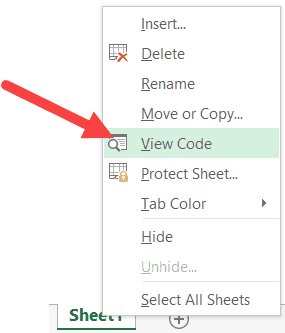
You need to copy and paste this code in the code window of the worksheet in which you need this functionality. To open the worksheet code window, left-click on the sheet name in the tabs and click on ‘View Code’
This is a good method when you need to manually scan a list and insert check marks. You can easily do this with a double click. The best use case of this is when you’re going through a list of tasks and have to mark it as done or not.
Click here to download the example file and follow along
Formatting the Check Mark Symbol
A check mark is just like any other text or symbol that you use.
This means that you can easily change its color and size.
All you need to do is select the cells that have the symbol and apply the formatting such as font size, font color, and bold etc.
This way of formatting symbols is manual and suited only when you have a couple of symbols to format. If you have a lot of these, it’s better to use conditional formatting to format these (as shown in the next section).
Format Check Mark / Cross Mark Using Conditional Formatting
With conditional formatting, you can format the cells based on what type of symbol it has.
Below is an example: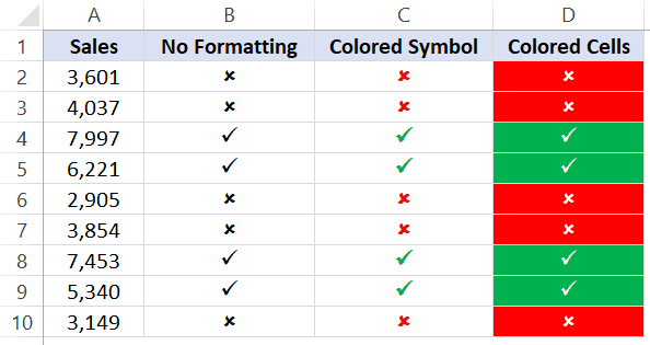
Column B uses the CHAR function to return a check mark if the value is more than 5000 and a cross mark if the value is less than 5000.
The ones in column C and D uses conditional formatting and look way better as it improves visual representation using colors.
Let’s see how you can do this.
Below is a dataset where I have used the CHAR function to get the check mark or cross mark based on the cell value.
Below are the steps to color the cells based on the symbol it has:
- Select the cells that have the check-mark/cross-mark symbols.
- Click the Home tab.
- Click on Conditional Formatting.
- Click on ‘New Rule’.
- In the New Formatting Rule dialog box, select ‘Use a formula to determine which cells to format’

- In the formula field, enter the following formula: =B2=CHAR(252)
- Click the Format button.
- In the ‘Format Cells’ dialog box, go to the Fill tab and select the green color.

- Go to the Font tab and select color as white (this is to make sure your checkmark looks nice when the cell has a green background color).
- Click OK.


After the above steps, the data is going to look as shown below. All the cells that have the check mark will be colored in green with white font.
You need to repeat the same steps to now format the cells with a cross mark. Change the formula to =B2=char(251) in step 6 and formatting in step 9.
Count Check Marks
If you want to count the total number of check marks (or cross marks), you can do that using a combination of COUNTIF and CHAR.
For example, suppose you have the data set as shown below and you want to find out the total number of stores that have achieved the sales target.
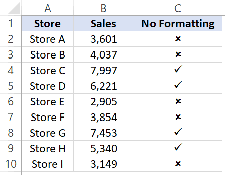
Below is the formula that will give you the total number of check marks in column C
=COUNTIF($C$2:$C$10,CHAR(252))
Note that this formula relies on you using the ANSI code 252 to get the check mark. This would work if you have used the keyboard shortcut ALT 0252, or have used the formula =Char(252) or have copied and pasted the check mark that is the created using these methods. If this is not the case, then the above COUNTIF function is not going to work.
You May Also like the following Excel tutorials:
- How to Insert Delta Symbol in Excel.
- How to Insert Degree Symbol in Excel.
- How to Insert a Line Break in Excel.
- How to Compare two columns in Excel.
- To-do List Excel Template.
Skip to content
Katarakyat.id
How to mark and color excel cells/ranges that contain certain text with Excel conditional formatting features automatically

Conditional Formatting of text in Excel
We have already learned about Excel how to mark cells containing specific numbers with features Conditional Formatting.
In this excel tutorial, we will learn about how to automatically mark or color Excel cells that contain text according to certain criteria.
Text Criteria In Excel Conditional Formatting
For text criteria, conditional formatting excel provides 4 (four) criteria models that we can apply.
- Containing: Marking Excel cells that contains / contains text certain.
- Not Containing: Marking Excel cells that does not contain / contain text certain.
- Beginning With: Marking Excel cells that beginning with text certain.
- Ending With: Marking Excel cells that ends with text certain.
As an example we will use the following data table:

From the data table above we want to change the color of cells automatically or Mark cells that contain text “Repeat“by color red fill. The steps we need to mark or color a cell with one of the four criteria above are :
- Selection of the data Range that we will mark (H2:H11)
- Select menu Home--Conditional Formatting--New Rule
- Select Format only cells that contain.
- On options Rule Description select Specific Text--Containing
- Enter text “Repeat“in the box next to it.
- Set the fill format to red or whatever you want.
- OK and done. Look at the results.
To better explain note the following pictures:


By applying conditional formatting above the result we get will be like this:

Now we try by applying rule Not Containing “without”.

The result that we will get by applying the conditional formatting above is as follows :

For other criteria you can try yourself. for example, giving rule Not Containing “repeat”, Beginning with “pass”, Containing “With”, etc.
I guess How to mark or color excel cells that match certain text criteria it’s very easy. so I don’t need to extend it anymore.
Still unclear? please submit in the comments field.
Thanks for visit my blog!
auto Cells Color Excel Mark Specific text Tutorial Excel
![]()
Download Article
![]()
Download Article
This wikiHow teaches you how to insert a checkmark icon into a cell in a Microsoft Excel document. While not all fonts support the checkmark icon, you can use the built-in Wingdings 2 font option to add a checkmark to any cell in Excel.
-

Click the cell into which you want to insert a checkmark. This highlights the cell.

Advertisement
-
You can find it on the Insert toolbar. Here’s how:
- Click the Insert tab at the top of Excel.
- Click the Symbols menu at the top-right corner.
- Click Symbol on the menu.

-
Click the «Font» menu and select Wingdings. This displays special characters you can insert into your spreadsheet.
- If you don’t see this font, use Segoe UI Symbol instead.[1]
- If you don’t see this font, use Segoe UI Symbol instead.[1]

Advertisement
-
Scroll through the characters and select the checkmark. Alternative, you can type 252 into the character code box (if using Wingdings) or 2714 (if using Segoe).

-
You’ll see the Insert button at the bottom of the window. This inserts the checkmark into the selected cell.

Advertisement
Ask a Question
200 characters left
Include your email address to get a message when this question is answered.
Submit
Advertisement
-
If you want to convert the entire Excel document font to Wingdings 2, click the Home tab, click the font drop-down box, scroll down in the drop-down menu, and click Wingdings 2 in the drop-down menu. This will allow you to copy and paste the checkmarks into other cells.
Thanks for submitting a tip for review!
Advertisement
-
Most fonts will not support the checkmark symbol. If you ever change the entire Excel document’s font to something other than Wingdings 2, your checkmarks will most likely disappear.
Advertisement
References
About This Article
Thanks to all authors for creating a page that has been read 123,990 times.
Is this article up to date?
Keep up with tech in just 5 minutes a week!
Subscribe
You’re all set!
Is there any way to declare a cell/row in Excel as a cell/row that should not be used for page break.
Example:
A1: 1. My content title in bold
A2: Empty row
A3: More and more content, description, etc...on many lines.
A4: 2. My other content title in bold
A5: Empty row
A6: More and more content, description, etc...on many lines.
If that goes on for many pages, I would like Excel not to break between A1 and A3, A4 and A6, etc.
Is that feasible?
asked Sep 8, 2010 at 15:09
![]()
The easiest and most fool-proof way will be to manually assign page breaks. Go to:
View->Page Break Preview
On this view you can drag page breaks (the dotted lines) to where you want, both horizontally and vertically. Excel will automagically adjust the size of the text/cells/etc. to fit into your specified breaks.
answered Sep 8, 2010 at 15:14
![]()
JNKJNK
8,17827 silver badges31 bronze badges
3
Last week while traveling I met a person who asked me a smart question. He was quietly working on his laptop and suddenly asked me this:
“Hey, do you know how to insert a check mark symbol in Excel?“
And then I figured out that he had a list of customers and he wanted to add a checkmark for every customer to whom he met.
Well, I showed him a simple way and he was happy with that. But eventually today morning, I thought maybe there is more than one way to insert a checkmark in a cell.
And luckily, I found that there several for this. So today in this post, I’d like to show you how to add a check mark symbol in Excel using 10 different methods and all those situations where we need to use these methods.
Apart from these 10 methods, I have also mentioned how you can format a checkmark + count checkmarks from a cell of the range.
Quick Notes
- In Excel, a checkmark is a character of wingding font. So, whenever you insert it in a cell that cell needs to have a wingding font style (Except, if you copy it from anywhere else).
- These methods can be used in all the Excel versions (2007, 2010, 2013, 2016, 2019, and Office 365).
download this sample file
When You should be using a Check Mark in Excel
A checkmark or tick is a mark that can be used to indicate the “YES”, to mention “Done” or “Complete”.
So, if you are using a to-do list, want to mark something is done, complete, or checked then the best way to use a checkmark.
1. Keyboard Shortcut to Add a Checkmark
Nothing is faster than a keyboard shortcut, and to add a checkmark symbol all you need a keyboard shortcut.
The only thing you need to take care of; The cell where you want to add the symbol must have wingding as font style. And below is the simple shortcut you can use insert a checkmark in a cell.
- If you are using Windows, then: Select the cell where you want to add it.
- Use Alt + 0 2 5 2 (make sure to hold the Alt key and then type “0252” with your numeric keypad).
- And, if you are using a Mac: Just select the cell where you want to add it.
- Use Option Key + 0 2 5 2 (make sure to hold the key and then type “0252” with your numeric keypad).


2. Copy Paste a Checkmark Symbol in a Cell
If you usually don’t use a checkmark then you can copy-paste it from somewhere and insert it in a cell
Because you are not using any formula, shortcut, or VBA here (copy paste a checkmark from here ✓).
Or you can also copy it by searching it on google. The best thing about the copy-paste method is there is no need to change the font style.
3. Insert a Check Mark Directly from Symbols Options
There are a lot of symbols in Excel which you can insert from the Symbols option, and the checkmark is one of them.
From Symbols, inserting a symbol in a cell is a brainer, you just need to follow the below steps:
- First, you need to select the cell where you want to add it.
- After that, go to Insert Tab ➜ Symbols ➜ Symbol.
- Once you click on the symbol button, you will get a window.
- Now from this window, select “Winding” from the font dropdown.
- And in the character code box, enter “252”.
- By doing this, it will instantly select the checkmark symbol and you don’t need to locate it.
- In the end, click on “Insert” and close the window.


As this is a “Winding” font, and the moment you insert it in a cell Excel changes the cell font style to “Winding”.
Apart from a simple tick mark, there is also a boxed checkmark is there (254) which you can use.
If you want to insert a tick mark symbol in a cell where you already have text, then you need to edit that cell (use F2).
The above method is a bit long, but you don’t have to use any formula or a shortcut key and once you add it into a cell you can copy-paste it.
4. Create an AUTOCORRECT to Convent it to a Check Mark
After the keyboard shortcut, the fast way is to add a checkmark/tick mark symbol in the cell, it’s by creating AUTOCORRECT.
In Excel, there is an option that corrects misspelled words. So, when you insert “clear” it converts it into “Clear” and that’s the right word.
Now thing is, it gives you the option to create an AUTOCORRECT for a word and you define a word for which you want Excel to convert it into a checkmark.
Below are the steps you need to use:
- First, go to the File Tab and open the Excel options.
- After that, navigate to “Proofing” and open the AutoCorrect Option.
- Now in this dialog box, in the “Replace” box, enter the word you want to type for which Excel will return a checkmark symbol (here I’m using CMRK).
- Then, in the “With:” enter the checkmark which you can copy from here.
- In the end, click OK.


From now, every time when you enter CHMRK Excel will convert it into an actual check mark.
There are a few things you need to take care which you this auto corrected check mark.
- When you create an auto-correct you need to remember that it’s case-sensitive. So, the best way can be to create two different auto corrects using the same word.
- The word you have specified to be corrected as a checkmark will only get converted if you enter it as a separate word. Let’s say if you enter Task1CHMRK it will not get converted as Task1. So, the text must be Task1 CHMRK.
- The AUTO correct option applied to all the Office Apps. So, when you create a autocorrect for a checkmark you can use it in other apps as well.
5. Macro to Insert a Checkmark in a Cell
If you want to save your efforts and time, then you can use a VBA code to insert a checkmark. Here is the code:
Sub addCheckMark()

Dim rng As Range

For Each rng In Selection
With rng
.Font.Name = "Wingdings"
.Value = "ü"
End With
Next rng

End Sub
Pro Tip: To use this code in all the files you add it into your Personal Macro Workbook.
Here’s how this code works.
When you select a cell or a range of cell and run this code it loops through each of the cells and changes its font style to “Wingdings” and enter value “ü” in it.
Top 100 Macro Codes for Beginners
Add Macro Code to QAT
This is a PRO tip that you can use if you are likely to use this code more often in your work. Follow these simple steps for this:
- First, click on the down arrow on the “Quick Access Toolbar” and open the “More Commands”.
- Now, from the “Choose Commands From” select the “Macros” and click on the “Add>>” to add this macro code to the QAT.
- In the end, click OK.
Double-Click Method using VBA
Let’s say you have a to-do list where you want to insert a checkmark just by double-clicking on the cell.
Well, you can make this happen by using VBA’s double-click event. Here I’m using the same code below code:
Private Sub Worksheet_BeforeDoubleClick(ByVal Target As Range, Cancel As Boolean)
If Target.Column = 2 Then
Cancel = True
Target.Font.Name = "Wingdings"
If Target.Value = "" Then
Target.Value = "ü"
Else
Target.Value = ""
End If
End If
End Sub
How to use this code
- First, you need to open the VBA code window of the worksheet and for this right-click on the worksheet tab and select the view code.
- After that, paste this code there and close the VB editor.
- Now, come back to the worksheet and double click on any cell in column B to insert a checkmark.

How this code works
When you double click on any cell this code triggers and check if the cell you on which you have double clicked is in column 2 or not.
And, if that cell is from column 2 change its font style to “Winding” after that it checks if that cell is blank or not, if the cell is blank then enter the value “ü” in it which converts into a checkmark as it has already applied the font style to the cell.
And if a cell has a checkmark already then you remove it by double-clicking.
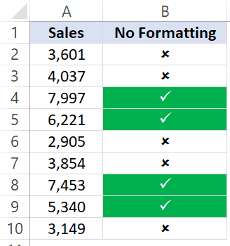
6. Add Green Check Mark with Conditional Formatting
If you want to be more awesome and creative, you can use conditional formatting for a checkmark.
Let’s say, below is the list of the tasks you have where you have a task in the one column and a second where you want to insert a tick mark if the task is completed.
Below are the steps you need to follow:
- First, select the target cell or range of cells where you want to apply the conditional formatting.
- After that go to Home Tab ➜ Styles ➜ Conditional Formatting ➜ Icon Sets ➜ More Rules.
- Now in the rule window, do the following things:
- Select the green checkmark style from the icon set.
- Tick mark the “Show icon only” option.
- Enter “1” as a value for the green checkmark and select a number from the type.
- In the end, click OK.

Once you do that, enter 1 in the cell where you need to enter a checkmark, and because of conditional formatting, you will get a green checkmark there without the actual cell value.

If you want to apply this formatting from one cell or range to another range you can do it by using format painter.
7. Create a Dropdown to Insert a Checkmark
If you don’t want to copy-paste checkmark and don’t even want to add the formula, then the better way can be to create a drop-down list using data validation and insert a checkmark using that drop-down.
Before you start make sure to copy a checkmark ✓ symbol before you start and then select the cell where you want to create this dropdown. And after that follow these simple steps to create a drop-down for adding a checkmark:
If you want to add a cross symbol ✖ along with the tick mark so that you can use any of them when you need simply add a cross symbol using a comma and click OK.
There’s one more benefit that drops down gives that you can disallow any other value in the cell other than a checkmark and a cross mark.
All you need to do is go to the “Error Alert” tab and tick mark “Show error alert after invalid data is entered” after that select the type, title, and a message to show when a different value is entered.
Related
- How to Create a Dependent Dropdown List in Excel
- How to Create a Dynamic Dropdown List in Excel
8. Use CHAR Function
Not all the time you need to enter a checkmark by yourself. You can automate it by using a formula as well. Let’s say you want to insert a checkmark based on a value in another cell.
Like below where when you enter value done in column C the formula will return a tick mark in column A. To create a formula like this we need to use CHAR function.
CHAR(number)

Related: Excel’s Formula Bar
Quick INTRO: CHAR Function
CHAR function returns the character based on the ASCII value and Macintosh character set.
Syntax:
CHAR(number)
…how does it work
As I say CHAR is a function to convert a number into an ANSI character (Windows) and Macintosh character set (Mac). So, when you enter 252 which is the ANSI code for a checkmark, the formula returns a checkmark.
9. Graphical Checkmark
If you are using OFFICE 365 like me, you can see there is a new tab with the name “Draw” there on your ribbon.

Now the thing is: In this tab, you have the option to draw directly into your spreadsheet. There are different pens and markers which you can use.
And you can simply draw a simple checkmark and Excel will insert it as a graphic.
The best thing is when you share it with others, even if they are using a different version of Excel, it shows as a graphic. There’s also a button to erase as well. You must go ahead and explore this “Draw” tab there is a lot of cool things which you can do with it.
10. Use Checkbox as a Checkmark in a Cell
You can also use a checkbox as a checkmark. But there is a slight difference between both:
- A checkbox is an object which is like a layer which placed above the worksheet, but a checkmark is a symbol which you can insert inside a cell.
- A checkbox is a sperate object and if you delete content from a cell checkbox won’t be deleted with it. On the other hand, a checkmark is a symbol which you inside a cell.
Here’s the detailed guide which can help you to learn more about a checkbox and using it in a right way.
11. Insert a Checkmark (Online)
If you use Excel’s online App then you need to follow a different way to put a checkmark in a cell.
The thing is, you can use the shortcut key but there is no “Winding” font there, so you can’t convert it into a checkmark. Even if you use the CHAR function it won’t be converted into a checkmark.
But…But…But…
I’ve found a simple way by installing an app into the Online Excel for symbols to insert check marks. Below are the steps you need to follow:
Yes, that’s it.
…make sure to get this sample file from here to follow along and try it yourself
Some of the IMPORTANT Points YOU need to learn
Here are a few points which you need to learn about using checkmark.
1. Formatting a Checkmark
Formatting a check mark can be required sometimes especially when you are working with data where you are validating something. Below are the things which you can do with a checkmark:
- Make it bold and italic.
- Change its color.
- Increase and decrease font size.
- Apply an underline.
2. Deleting a Checkmark
Deleting a check mark is simple and all you need to do is select the cell where you have it and press the delete key.
Or, if you have text along with a checkmark in a cell then you can use any of the below methods.
- First, edit the cell (F2) and delete the checkmark.
- Second, replace the checkmark with no character using find and replace option.
3. Count Checkmarks
Let’s say want to count the checkmark symbols you have in a range of cells. Well, you need to use formula by combining COUNTIF and CHAR and the formula will be:
=COUNTIF(G3:G9,CHAR(252))
In this formula, I have used COUNTIF to count the characters which are returned by the CHAR.
…make sure to check this sample file from here to follow along and try it yourself
In the End,
A check mark is helpful when you are managing lists.
And creating a list with checkmarks in Excel is no big deal now, as you know more than 10 methods for this. From all the methods above, I always love to use conditional formatting……and sometimes copy-paste.
You can use any of these which you think is perfect for you. I hope this tip will help you in your daily work. But now tell me one thing.
Have you ever used any of the above methods? Which method is your favorite?
Make sure to share your views with me in the comment section, I’d love to hear from you. And please, don’t forget to share this post with your friends, I am sure they will appreciate it.
read these tutorials next…
- Add Leading Zeros in Excel
- Bullet Points in Excel
- Insert Checkbox in Excel
- Insert/Type Degree Symbol
- Serial Number Column
- Strikethrough
- Insert Delta Symbol
- SQUARE ROOT
- Remove Extra Spaces