Макрос для среднего значения в excel

This tutorial will demonstrate how to use the Excel Average function in VBA.

The Excel AVERAGE Function is used to calculate an average from a range cells in your Worksheet that have values in them. In VBA, It is accessed using the WorksheetFunction method.

AVERAGE WorksheetFunction

The WorksheetFunction object can be used to call most of the Excel functions that are available within the Insert Function dialog box in Excel. The AVERAGE function is one of them.

Sub TestFunction
  Range("D33") = Application.WorksheetFunction.Average("D1:D32")
End Sub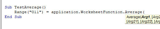

You are able to have up to 30 arguments in the AVERAGE  function. Each of the arguments must refer to a range of cells.

This example below will produce the average of the sum of the cells B11 to N11

Sub TestAverage()
   Range("O11") = Application.WorksheetFunction.Average(Range("B11:N11"))
End Sub

The example below will produce an average of the sum of the cells in B11 to N11 and the sum of the cells in B12:N12. If you do not type the Application object, it will be assumed.

Sub TestAverage()
  Range("O11") = WorksheetFunction.Average(Range("B11:N11"),Range("B12:N12")) 
End Sub

Assign AVERAGE Result to a Variable

You may want to use the result of your formula elsewhere in code rather than writing it directly back to an Excel Range. If this is the case, you can assign the result to a variable to use later in your code.

Sub AssignAverage()
   Dim result As Integer
'Assign the variable   
   result = WorksheetFunction.Average(Range("A10:N10"))
'Show the result
   MsgBox "The average for the cells in this range is " & result
End Sub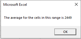

AVERAGE with a Range Object

You can assign a group of cells to the Range object, and then use that Range object with the WorksheetFunction object.

Sub TestAverageRange()
   Dim rng As Range
'assign the range of cells
   Set rng = Range("G2:G7")
'use the range in the  formula
   Range("G8") = WorksheetFunction.Average(rng)
'release the range object
  Set rng = Nothing
End Sub

AVERAGE Multiple Range Objects

Similarly, you can calculate the average of the cells from multiple Range Objects.

Sub TestAverageMultipleRanges() 
   Dim rngA As Range 
   Dim rngB as Range
'assign the range of cells 
   Set rngA = Range("D2:D10") 
   Set rngB = Range("E2:E10")   
'use the range in the formula 
Range("E11") = WorksheetFunction.Average(rngA, rngB)
 'release the range object
  Set rngA = Nothing 
  Set rngB = Nothing
End Sub

Using AVERAGEA

The AVERAGEA Function differs from the AVERAGE function in that it create an average from all the cells in a range, even if one of the cells has text in it – it replaces the text with a zero and includes that in calculating the average.   The AVERAGE function would ignore that cell and not factor it into the calculation.

Sub TestAverageA()
   Range("B8) = Application.WorksheetFunction.AverageA(Range("A10:A11")) 
End Sub

In the example below, the AVERAGE function returns a different value to the AVERAGEA function when the calculation is used on cells A10 to A11

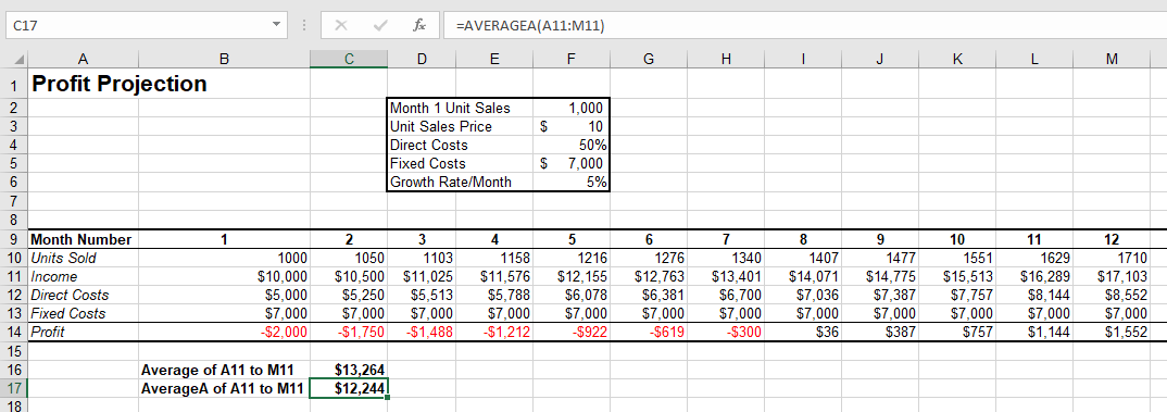
The answer for the AVERAGEA formula is lower than the AVERAGE formula as it replaces the text in A11 with a zero, and therefore averages over 13 values rather than the 12 values that the AVERAGE is calculating over.

Using AVERAGEIF

The AVERAGEIF Function allows you to average the sum of a range of cells that meet a certain criteria.

Sub AverageIf()
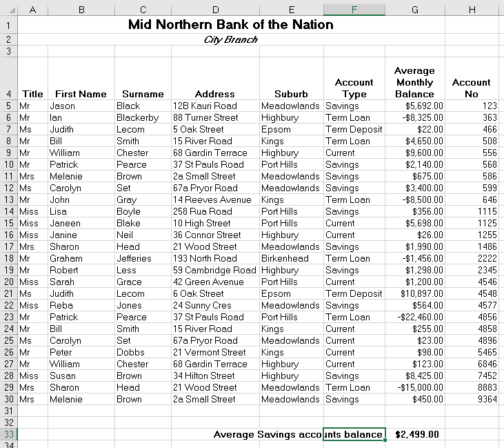
   Range("F31") = WorksheetFunction.AverageIf(Range("F5:F30"), "Savings", Range("G5:G30"))
End Sub

The procedure above will only average the cells in range G5:G30 where the corresponding cell in column F has the word ‘Savings’ in it.  The criteria you use has to be in quotation marks.

Disadvantages of WorksheetFunction

When you use the WorksheetFunction to average the values in a range in your worksheet, a static value is returned, not a flexible formula. This means that when your figures in Excel change, the value that has been returned by the WorksheetFunction will not change.

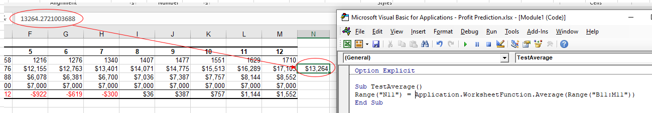
In the example above, the procedure TestAverage procedure has created the average of B11:M11 and put the answer in N11.   As you can see in the formula bar, this result is a figure and not a formula.

If any of the values change therefore in the Range(B11:M11 ), the results in N11 will NOT change.

Instead of using the WorksheetFunction.Average, you can use VBA to apply the AVERAGE Function to a cell using the Formula or FormulaR1C1 methods.

Using the Formula Method

The formula method allows you to point specifically to a range of cells eg: B11:M11 as shown below.

Sub TestAverageFormula()
  Range("N11").Formula = "=Average(B11:M11)"
End Sub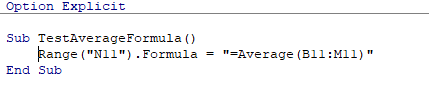

Using the FormulaR1C1 Method

The FomulaR1C1 method is more flexible in that it does not restrict you to a set range of cells. The example below will give us the same answer as the one above.

Sub TestAverageFormula()
   Range("N11").Formula = "=Average(RC[-12]:RC[-1])"
End Sub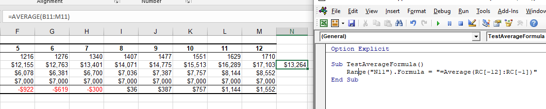

However, to make the formula more flexible, we could amend the code to look like this:

Sub TestAverageFormula() 
   ActiveCell.FormulaR1C1 = "=Average(R[-11]C:R[-1]C)" 
End Sub

Wherever you are in your worksheet, the formula will then average the values in the 12 cells directly to the left of it and place the answer into your ActiveCell. The Range inside the AVERAGE function has to be referred to using the Row (R) and Column (C) syntax.

Both these methods enable you to use Dynamic Excel formulas within VBA.

There will now be a formula in N11 instead of a value.

In Excel, you can use VBA to calculate the average values from a range of cells or multiple ranges. And, in this tutorial, we are going to learn the different ways that we can use it.

Average in VBA using WorksheetFunction

In VBA, there are multiple functions that you can use, but there’s no specific function for this purpose. That does not mean we can’t do an average. In VBA, there’s a property called WorksheetFunction that can help you to call functions into a VBA code.

Let’s average values from the range A1:A10.

1. First, enter the worksheet function property and then select the AVERAGE function from the list.
   
2. Next, you need to enter starting parenthesis as you do while entering a function in the worksheet.
   
3. After that, we need to use the range object to refer to the range for which we want to calculate the average.
   
4. In the end, type closing parenthesis and assign the function’s returning value to cell B1.
   

Application.WorksheetFunction.Average(Range("A1:A10"))

Now when you run this code, it will calculate the average for the values that you have in the range A1:A10 and enter the value in cell B1.

Average Values from an Entire Column or a Row

In that case, you just need to specify a row or column instead of the range that we have used in the earlier example.

'for the entire column A
Range("B1") = Application.WorksheetFunction.Average(Range("A:A"))

'for entire row 1
Range("B1") = Application.WorksheetFunction.Average(Range("1:1"))

Use VBA to Average Values from the Selection

Now let’s say you want to average value from the selected cells only in that you can use a code just like the following.

Sub vba_average_selection()

Dim sRange As Range
Dim iAverage As Long

On Error GoTo errorHandler

Set sRange = Selection

iAverage = WorksheetFunction.Average(Range(sRange.Address))
MsgBox iAverage

Exit Sub

errorHandler:
MsgBox "make sure to select a valid range of cells"

End Sub

In the above code, we have used the selection and then specified it to the variable “sRange” and then use that range variable’s address to get the average.

VBA Average All Cells Above

The following code takes all the cells from above and average values from them and enters the result in the selected cell.

Sub vba_auto_Average()

Dim iFirst As String
Dim iLast As String
Dim iRange As Range

On Error GoTo errorHandler

iFirst = Selection.End(xlUp).End(xlUp).Address
iLast = Selection.End(xlUp).Address

Set iRange = Range(iFirst & ":" & iLast)
ActiveCell = WorksheetFunction.Average(iRange)

Exit Sub

errorHandler:
MsgBox "make sure to select a valid range of cells"

End Sub

Average a Dynamic Range using VBA

And in the same way, you can use a dynamic range while using VBA to average values.

Sub vba_dynamic_range_average()

Dim iFirst As String
Dim iLast As String
Dim iRange As Range

On Error GoTo errorHandler

iFirst = Selection.Offset(1, 1).Address
iLast = Selection.Offset(5, 5).Address

Set iRange = Range(iFirst & ":" & iLast)
ActiveCell = WorksheetFunction.Average(iRange)

Exit Sub

errorHandler:
MsgBox "make sure to select a valid range of cells"

End Sub

Average a Dynamic Column or a Row

In the same way, if you want to use a dynamic column you can use the following code where it will take the column of the active cell and average for all the values that you have in it.

Sub vba_dynamic_column()

Dim iCol As Long

On Error GoTo errorHandler

iCol = ActiveCell.Column
MsgBox WorksheetFunction.Average(Columns(iCol))

Exit Sub

errorHandler:
MsgBox "make sure to select a valid range of cells"

End Sub

And for a row.

Sub vba_dynamic_row()

Dim iRow As Long

On Error GoTo errorHandler

iRow = ActiveCell.Row

MsgBox WorksheetFunction.Average(Rows(iCol))

Exit Sub

errorHandler:
MsgBox "make sure to select a valid range of cells"

End Sub

Perform a Vlookup that returns the highest value, lowest value, or average value from a dataset.

Sections:

Vlookup to Return Max

Vlookup to Return Min

Vlookup to Return Average

Notes

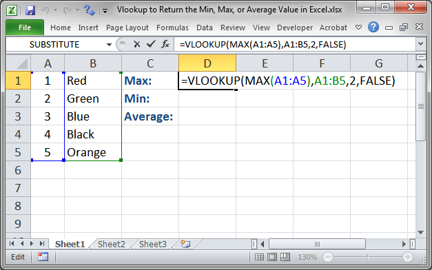
Vlookup to Return Max

Return the max value from a table of data.

=VLOOKUP(MAX(A1:A5),A1:B5,2,FALSE)

Result:

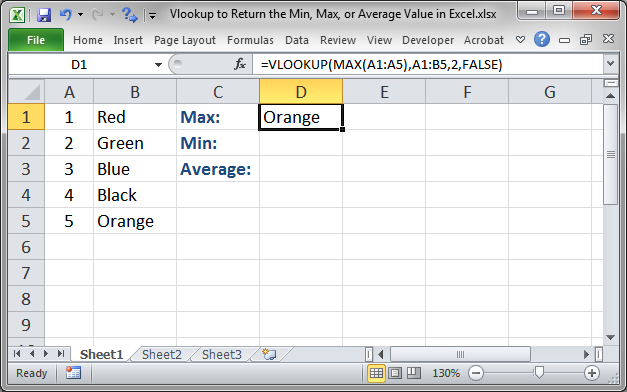
This Vlookup function is exactly the same as the regular one except that the MAX() function is used for the lookup value argument.

The MAX() function returns the highest value from the list of numbers and then that value is used to perform the lookup. Otherwise, this is a standard Vlookup function.

Vlookup to Return Min

Return the min value from a table of data.

=VLOOKUP(MIN(A1:A5),A1:B5,2,FALSE)

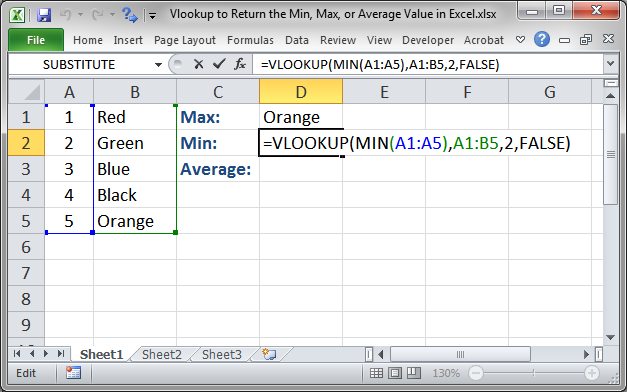
Result:

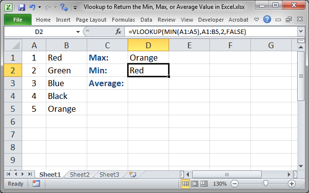
The MIN() function is used in this example to find the smallest value from the list of numbers; then, that value is used to perform the lookup in the lookup_value argument. Otherwise, this is a standard Vlookup function.

Vlookup to Return Average

Return the average value from a table of data.

=VLOOKUP(AVERAGE(A1:A5),A1:B5,2,TRUE)

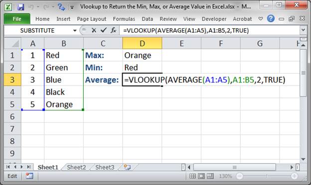
Result:

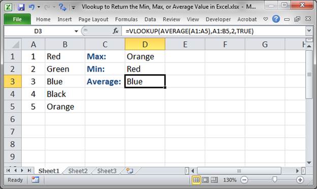
The AVERAGE() function is used in the lookup_value argument in order to find the average value from the list of numbers; then, that value, which is the average, is used to perform the lookup.

Note: in this example the last argument, range_lookup, is set to TRUE. This is because the average function can return a value that is not in the list of values and so you need the Vlookup function to find the next highest value. In this example, it doesn’t matter, but, if you want to check it out, change the 5 in row 5 to 12 and the TRUE value in cell D3 to FALSE and you will get an #N/A error.

Notes

Vlookups can be really helpful once you get used to using them and this is just one more way you can make them work for you to quickly return relevant and useful data.

Make sure to download the sample file for this tutorial so you can work with these examples in Excel.

Similar Content on TeachExcel

Subscribe for Weekly Tutorials

BONUS: subscribe now to download our Top Tutorials Ebook!