Making button in excel

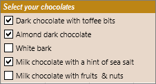
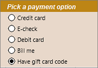
You can insert form controls such as check boxes or option buttons to make data entry easier. Check boxes work well for forms with multiple options. Option buttons are better when your user has just one choice.

To add either a check box or an option button, you’ll need the Developer tab on your Ribbon.

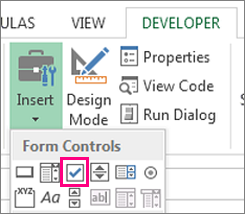
1. To add a check box, click the Developer tab, click Insert, and under Form Controls, click .

   

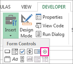
   To add an option button, click the Developer tab, click Insert, and under Form Controls, click .

   

2. Click in the cell where you want to add the check box or option button control.

   Tip: You can only add one checkbox or option button at a time. To speed things up, after you add your first control, right-click it and select Copy > Paste.

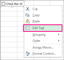
3. To edit or remove the default text for a control, click the control, and then update the text as needed.

   

Tip: If you can’t see all of the text, click and drag one of the control handles until you can read it all. The size of the control and its distance from the text can’t be edited.

Formatting a control

After you insert a check box or option button, you might want to make sure that it works the way you want it to. For example, you might want to customize the appearance or properties.

Note: The size of the option button inside the control and its distance from its associated text cannot be adjusted.

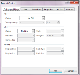
1. To format a control, right-click the control, and then click Format Control.

   

2. In the Format Control dialog box, on the Control tab, you can modify any of the available options:

   • Checked: Displays an option button that is selected.

   • Unchecked: Displays an option button that is cleared.

   • In the Cell link box, enter a cell reference that contains the current state of the option button.

     The linked cell returns the number of the selected option button in the group of options. Use the same linked cell for all options in a group. The first option button returns a 1, the second option button returns a 2, and so on. If you have two or more option groups on the same worksheet, use a different linked cell for each option group.

     Use the returned number in a formula to respond to the selected option.

     For example, a personnel form, with a Job type group box, contains two option buttons labeled Full-time and Part-time linked to cell C1. After a user selects one of the two options, the following formula in cell D1 evaluates to «Full-time» if the first option button is selected or «Part-time» if the second option button is selected.

     =IF(C1=1,»Full-time»,»Part-time»)

     If you have three or more options to evaluate in the same group of options, you can use the CHOOSE or LOOKUP functions in a similar manner.

3. Click OK.

Deleting a control

• Right-click the control, and press DELETE.

Currently, you can’t use check box controls in Excel for the web. If you’re working in Excel for the web and you open a workbook that has check boxes or other controls (objects), you won’t be able to edit the workbook without removing these controls.

Important: If you see an «Edit in the browser?» or «Unsupported features» message and choose to edit the workbook in the browser anyway, all objects such as check boxes, combo boxes will be lost immediately. If this happens and you want these objects back, use Previous Versions to restore an earlier version.

If you have the Excel desktop application, click Open in Excel and add check boxes or option buttons.

Содержание

• Процедура создания
  • Способ 1: автофигура
  • Способ 2: стороннее изображение
  • Способ 3: элемент ActiveX
  • Способ 4: элементы управления формы
• Вопросы и ответы

Excel является комплексным табличным процессором, перед которым пользователи ставят самые разнообразные задачи. Одной из таких задач является создание кнопки на листе, нажатие на которую запускало бы определенный процесс. Данная проблема вполне решаема с помощью инструментария Эксель. Давайте разберемся, какими способами можно создать подобный объект в этой программе.

Процедура создания

Как правило, подобная кнопка призвана выступать в качестве ссылки, инструмента для запуска процесса, макроса и т.п. Хотя в некоторых случаях, данный объект может являться просто геометрической фигурой, и кроме визуальных целей не нести никакой пользы. Данный вариант, впрочем, встречается довольно редко.

Способ 1: автофигура

Прежде всего, рассмотрим, как создать кнопку из набора встроенных фигур Excel.

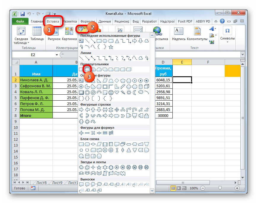
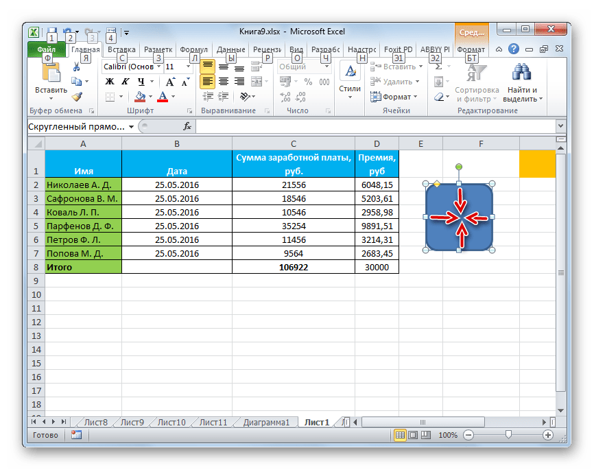
1. Производим перемещение во вкладку «Вставка». Щелкаем по значку «Фигуры», который размещен на ленте в блоке инструментов «Иллюстрации». Раскрывается список всевозможных фигур. Выбираем ту фигуру, которая, как вы считаете, подойдет более всего на роль кнопки. Например, такой фигурой может быть прямоугольник со сглаженными углами.



2. После того, как произвели нажатие, перемещаем его в ту область листа (ячейку), где желаем, чтобы находилась кнопка, и двигаем границы вглубь, чтобы объект принял нужный нам размер.



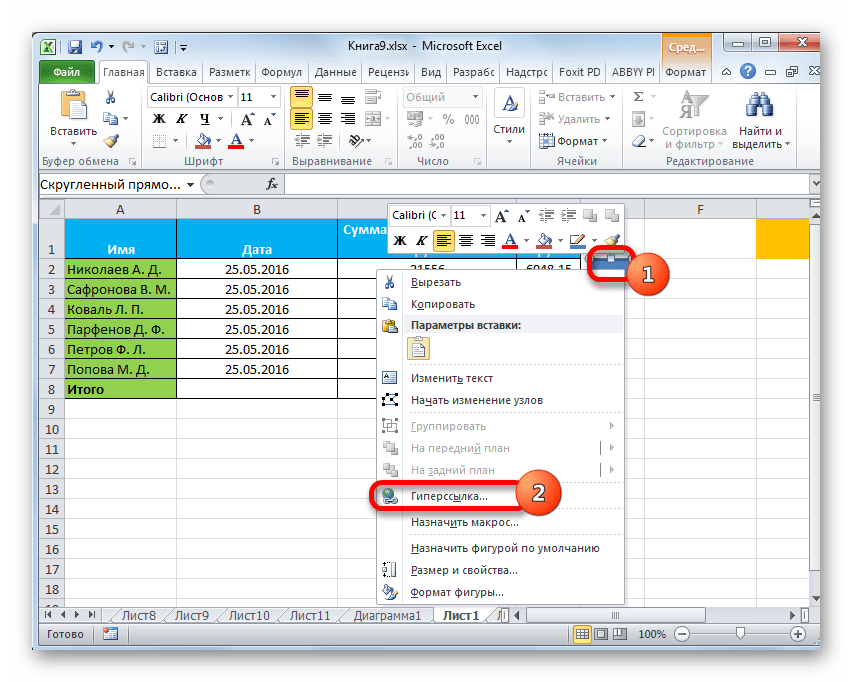
3. Теперь следует добавить конкретное действие. Пусть это будет переход на другой лист при нажатии на кнопку. Для этого кликаем по ней правой кнопкой мыши. В контекстном меню, которое активируется вслед за этим, выбираем позицию «Гиперссылка».



4. В открывшемся окне создания гиперссылки переходим во вкладку «Местом в документе». Выбираем тот лист, который считаем нужным, и жмем на кнопку «OK».

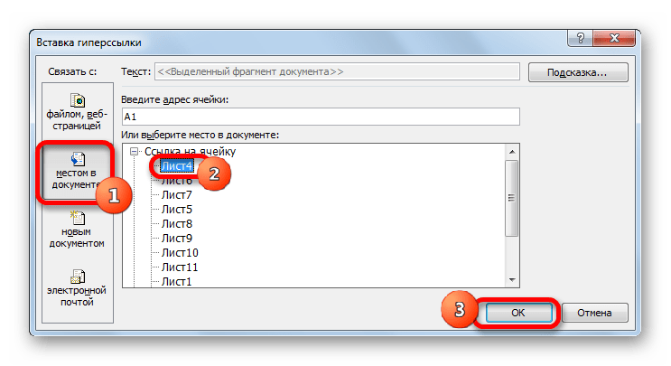
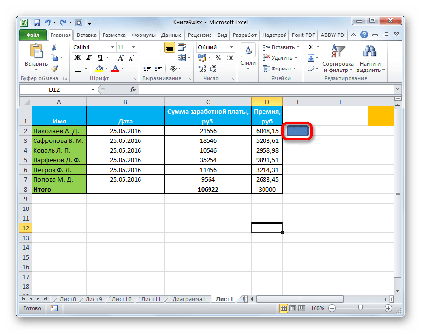
Теперь при клике по созданному нами объекту будет осуществляться перемещение на выбранный лист документа.

Урок: Как сделать или удалить гиперссылки в Excel

Способ 2: стороннее изображение

В качестве кнопки можно также использовать сторонний рисунок.

1. Находим стороннее изображение, например, в интернете, и скачиваем его себе на компьютер.
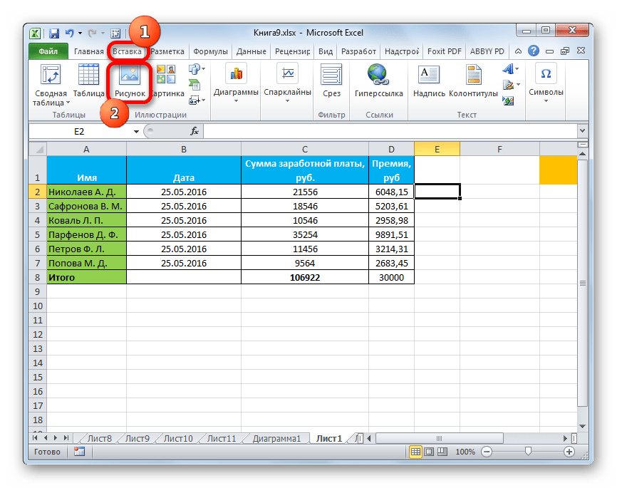
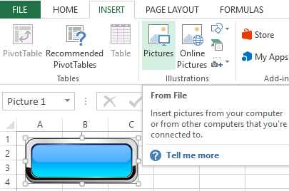
2. Открываем документ Excel, в котором желаем расположить объект. Переходим во вкладку «Вставка» и кликаем по значку «Рисунок», который расположен на ленте в блоке инструментов «Иллюстрации».



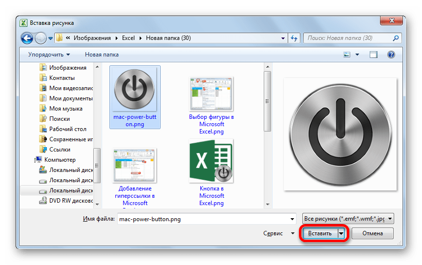
3. Открывается окно выбора изображения. Переходим с помощью него в ту директорию жесткого диска, где расположен рисунок, который предназначен выполнять роль кнопки. Выделяем его наименование и жмем на кнопку «Вставить» внизу окна.



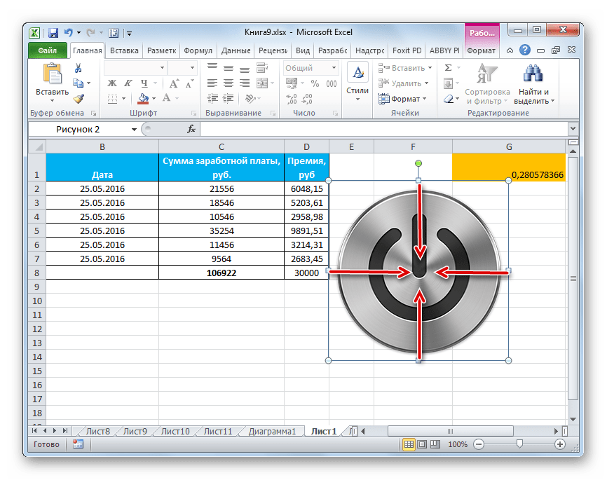
4. После этого изображение добавляется на плоскость рабочего листа. Как и в предыдущем случае, его можно сжать, перетягивая границы. Перемещаем рисунок в ту область, где желаем, чтобы размещался объект.





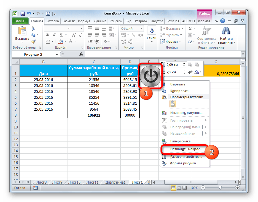
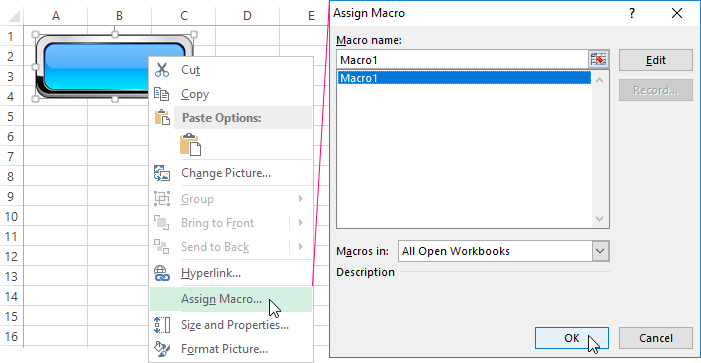
5. После этого к копке можно привязать гиперссылку, таким же образом, как это было показано в предыдущем способе, а можно добавить макрос. В последнем случае кликаем правой кнопкой мыши по рисунку. В появившемся контекстном меню выбираем пункт «Назначить макрос…».



6. Открывается окно управление макросами. В нем нужно выделить тот макрос, который вы желаете применять при нажатии кнопки. Этот макрос должен быть уже записан в книге. Следует выделить его наименование и нажать на кнопку «OK».

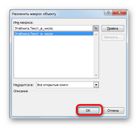
Теперь при нажатии на объект будет запускаться выбранный макрос.

Урок: Как создать макрос в Excel

Способ 3: элемент ActiveX

Наиболее функциональной кнопку получится создать в том случае, если за её первооснову брать элемент ActiveX. Посмотрим, как это делается на практике.

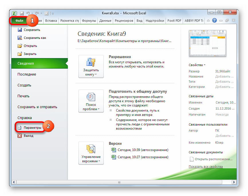
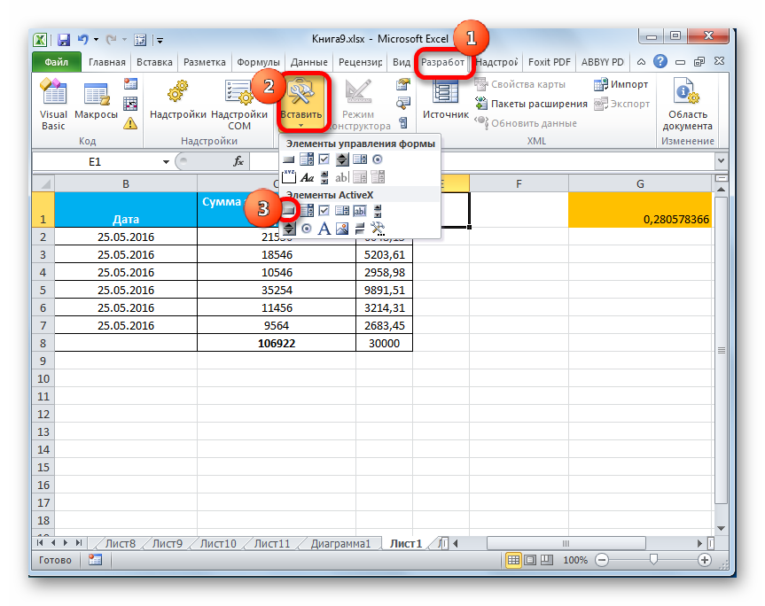
1. Для того чтобы иметь возможность работать с элементами ActiveX, прежде всего, нужно активировать вкладку разработчика. Дело в том, что по умолчанию она отключена. Поэтому, если вы её до сих пор ещё не включили, то переходите во вкладку «Файл», а затем перемещайтесь в раздел «Параметры».



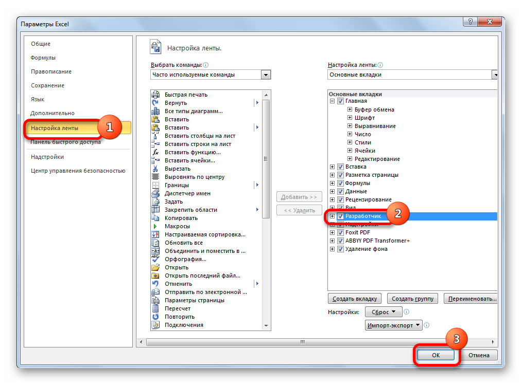
2. В активировавшемся окне параметров перемещаемся в раздел «Настройка ленты». В правой части окна устанавливаем галочку около пункта «Разработчик», если она отсутствует. Далее выполняем щелчок по кнопке «OK» в нижней части окна. Теперь вкладка разработчика будет активирована в вашей версии Excel.



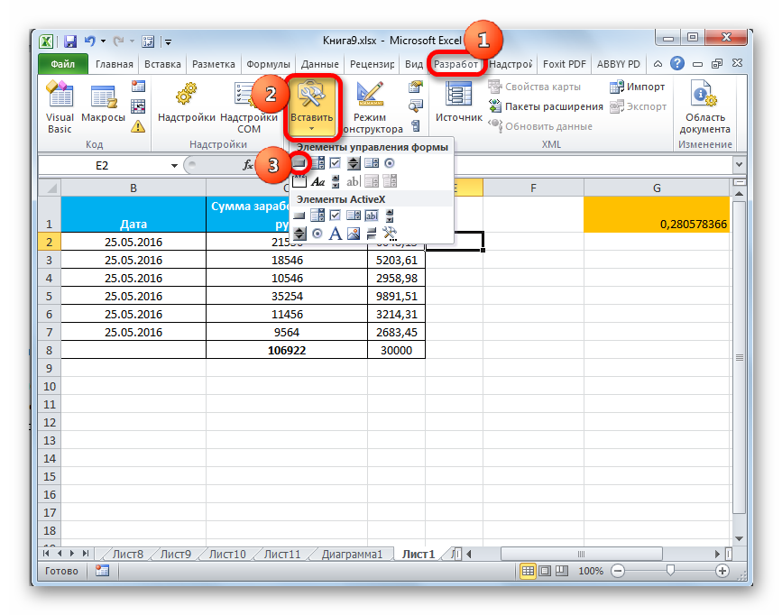
3. После этого перемещаемся во вкладку «Разработчик». Щелкаем по кнопке «Вставить», расположенной на ленте в блоке инструментов «Элементы управления». В группе «Элементы ActiveX» кликаем по самому первому элементу, который имеет вид кнопки.



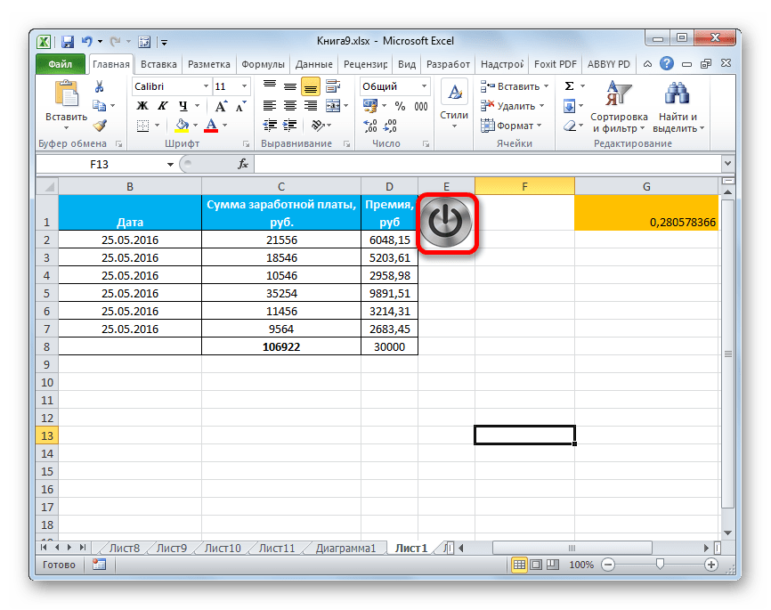
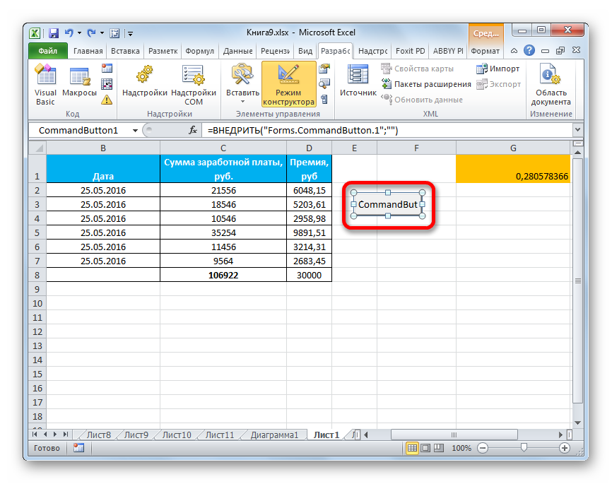
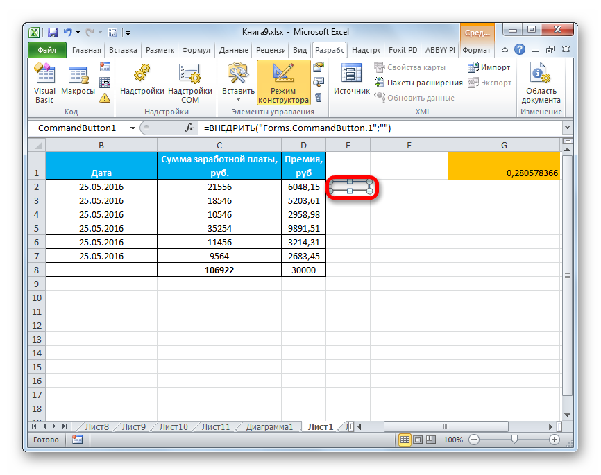
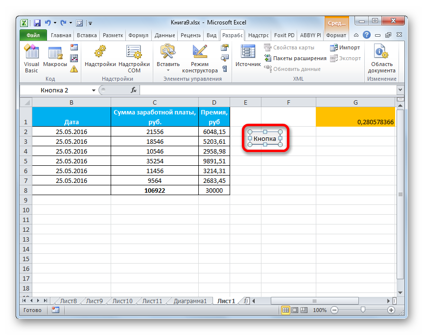
4. После этого кликаем по любому месту на листе, которое считаем нужным. Сразу вслед за этим там отобразится элемент. Как и в предыдущих способах корректируем его местоположение и размеры.



5. Кликаем по получившемуся элементу двойным щелчком левой кнопки мыши.



6. Открывается окно редактора макросов. Сюда можно записать любой макрос, который вы хотите, чтобы исполнялся при нажатии на данный объект. Например, можно записать макрос преобразования текстового выражения в числовой формат, как на изображении ниже. После того, как макрос записан, жмем на кнопку закрытия окна в его правом верхнем углу.

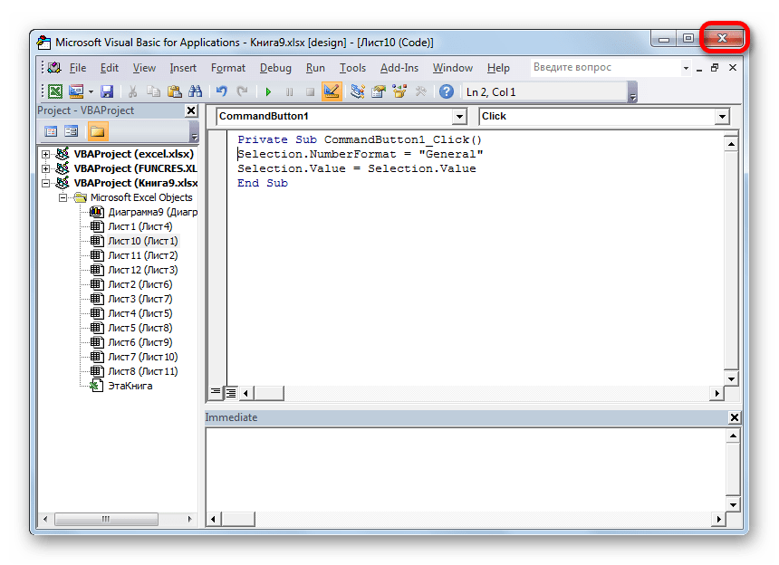
Теперь макрос будет привязан к объекту.

Способ 4: элементы управления формы

Следующий способ очень похож по технологии выполнения на предыдущий вариант. Он представляет собой добавление кнопки через элемент управления формы. Для использования этого метода также требуется включение режима разработчика.

1. Переходим во вкладку «Разработчик» и кликаем по знакомой нам кнопке «Вставить», размещенной на ленте в группе «Элементы управления». Открывается список. В нем нужно выбрать первый же элемент, который размещен в группе «Элементы управления формы». Данный объект визуально выглядит точно так же, как и аналогичный элемент ActiveX, о котором мы говорили чуть выше.



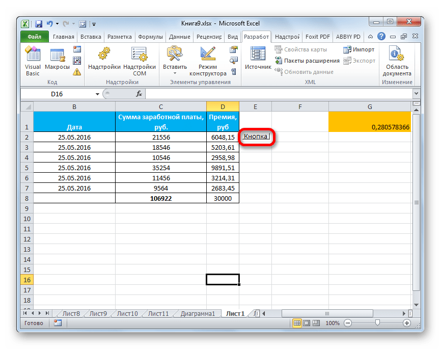
2. Объект появляется на листе. Корректируем его размеры и место расположения, как уже не раз делали ранее.



3. После этого назначаем для созданного объекта макрос, как это было показано в Способе 2 или присваиваем гиперссылку, как было описано в Способе 1.

Как видим, в Экселе создать функциональную кнопку не так сложно, как это может показаться неопытному пользователю. К тому же данную процедуру можно выполнить с помощью четырех различных способов на свое усмотрение.

Еще статьи по данной теме:

Помогла ли Вам статья?

Home / Excel Basics / How to Add a Button in Excel

In Excel, users can add macro-enabled buttons on the worksheets and can run macros by just clicking on them.

Users can use these macro-enabled buttons to perform several different tasks like filtering data, selecting data, printing a worksheet, running formulas, and calculations just by clicking on the buttons.

Adding buttons and embedding the macros to them is easier. Excel has multiple ways to add the macro-enabled buttons to the worksheet. Below, we have some quick and easy ways mentioned for you to add the macro buttons in Excel.

Add Macro Buttons Using Shapes

Users can create buttons in excel using shapes. Creating buttons using shapes has more formatting options over the buttons created from Control buttons or ActiveX buttons. Users can change the design, color, font, and style of the button created using shapes.

1. First, go to the “Insert” tab and then click on the “Illustrations” icon” then click on the “Shapes” option and select any rectangle button.
   
2. After that, with the help of a mouse, draw the rectangular button on the worksheet.
   
3.  Now, to enter the text in the button, double-click on the button and insert the text.
   
4. For formatting, go to the “Shape Format” tab and you will get multiple options for the formatting of the button.
5. From here, you can format the font style, font color, button color, button effects, and much more.
   
6. To edit the text, add the hyperlink, or add the macro, just right-click on the button and you will get the pop-up menu with multiple options.
7. From here, you can edit the text, add the hyperlink, and can add the macro to the button.
8. Now, select the “Assign Macro” option to add the macro to the button.
   
9. Once you select the “Assign Macro” option, you will get the “Assign Macro” dialogue box opened.
10. From here, select the macro and click OK.
    
11. At this point, the button has become micro enabled, and when you move your cursor on the button, the cursor turns to the hand point cursor.
    
12. To freeze the button movement, right-click on the button and select the “Format Shape” and select the option “Don’t move or size with cells”.
    

Add Macro Buttons Using Form Controls

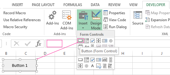
1. First, go to the “Developer” tab and click on the “Insert” icon under the “Control” group on the ribbon.
   
2. After that, select the first button option from the “Form Controls” menu and draw a button on the worksheet.
   
3. Now, select or type the macro name from the “Assign Macro” dialogue box and click OK.
4. If you don’t have any macro created yet, you can click cancel to add the macro at a later stage.
   
5. From here, right-click on the button and select “Assign Macro” to add the macro to the button if did not assign yet.
6. To format the button font size, style, color, etc. select the “Format Control” option.
   
7. Once you click on “Format Control”, you will get the “Format Control” window open and then can do the button font formatting.
   
8. To freeze the button movement, select the “Properties” tab and select the option “Don’t move or size with cells” and click OK.
   

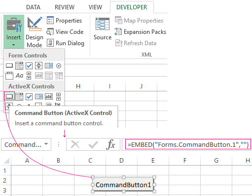
Add Macro Buttons Using ActiveX Controls

1. First, go to the “Developer” tab and click on the “Insert” icon under the “Control” group on the ribbon.
   
2. After that, select the first button option from the “ActiveX Controls” menu and draw a button on the worksheet.
   
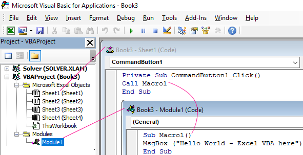
3. Now, to create and insert the macro to the button, click on the “View Code” icon to launch the VBA editor.
   
4. Now, select the” CommandButton1” on the subprocedure and choose the “Click” option from the drop-down list on the right side of the editor.
   

When we mention buttons in Excel, anyone who is not a consistent user will wonder what that means. Yes, Microsoft Excel does have Macros buttons which are the most advanced level of Excel. These buttons are commands initiated by a single click. It is easy to add buttons to excel. A user can simplify and save the time that they will take to navigate between different cells looking for specific information. In short, the buttons are inserted to perform specific tasks for us. The three different types of buttons you can place in a worksheet include;

• Shapes
• Form Control Buttons

This article shows how to add a button in Excel and how to assign Macros to them. With those buttons, navigating through your spreadsheet won’t be a nightmare anymore.

Method 1: Using shapes to create Macro buttons to open a particular sheet

You can create a macros button by using shapes. You can easily create a rounded rectangle; add a hyperlink to it for your worksheet. Here is what you can do;
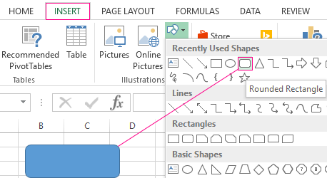
1. On the main menu ribbon, click on the Insert tab.

2. Go to Shapes, click the drop-down arrow, and select the Rounded Rectangle icon.

3. Draw a rounded rectangle on your worksheet.

5. Format the shape by typing text into it-Right-click on the form and select edit text. Or double-click the shape.

6. To Hyperlink the shape, right-click on it and select Hyperlink from the menu. Right-clicking will display an Insert Hyperlink dialogue box.

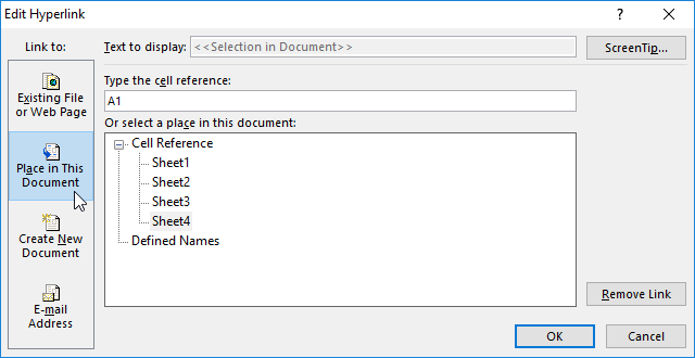
• Under the ‘Link to’ section, select ‘Place in This Document.
• Under the ‘Type the cell reference’ section, type in the destination cell address.
• Under the ‘Or select a place in this document box, click to choose the particular sheet name. Click the OK button when done.

When you click the rounded rectangle, it will skip to the specified cell of a specified sheet.

7. To assign the macro, right-click on the table and select Assign Macro. Under the ‘Macros in’ drop-down arrow, select ‘This Workbook’. Here, select the macro from the list of macros in This Workbook.

8. Press OK. When you point your mouse on this shape, it will turn to the hand pointer cursor, and clicking the form will run the macro. Remember to set your shape not to resize with cell changes by right-clicking on it and selecting ‘Size and Properties.’

Method 2: Using Developers Form Control Buttons to create buttons in Excel

1. On the main ribbon, click on the Developer tab.

2. Go to the Insert button and click the drop-down arrow.

3. Under Form Control, select the first option called button. Draw a button on your worksheet

4. Next, in the Assign Macro dialogue box, type or select a name for the macro.

5. Click OK when done. You can click on this button to run the macro.

Using ActiveX Controls

 Since running a macro in Excel can prove tedious, you can assign a macro to a button to run it faster. In this case, you can follow these steps to add a button in Excel using ActiveX controls easily.

1. Right-click anywhere on the Home ribbon and select Customize the Ribbon option from the pop-up menu. 

2. Once the Customize the Ribbon window is open, go to the Main Tabs section and select the Developer option.

3. Click OK. However, if you already have the Developer Tab added to your ribbon, then proceed as follows. 

4. Go to the Developer Tab and click on Insert.

5. Next, click on your preferred button under the ActiveX Controls.

You can now drag it anywhere in the Excel worksheet to create a button. 

6. Right-click on the newly created button and select the View Code option from the drop-down menu. 

7. You can now type this code, which sets the value of cell A6 to Hello:

Range(“A6”).Value = “Hello”

8. If you want to test setting the cell value, ensure the Design Mode option is deselected. You can also click on the button, and the Hello text will be displayed on your screen.

You can further use VBA codes to assign a different task for various operations such as double-clicking, single-clicking, right-clicking, and many more. When you right-click on the button, you can also select the Format Control option. However, the only downside is that the size of the buttons changes every time you make changes on the worksheet or share it.

Adding Macros To Quick Access Toolbar

Adding macros to Quick Access Toolbar also allows you to create buttons in Excel and use them on any sheet in your present workbook. To do this, follow these steps:

1. Right-click on the arrow below the ribbon of the Excel workbook.

2. When the Customize Quick Access Toolbar screen opens, navigate and select More Commands at the bottom.

3. Select Macros in the Choose commands from the section. You can click on the down-facing arrow in the Popular Commands box.

4. Select the HighlightMaxValue option and click on the Add button.

5. You can now click on Modify to customize the symbol of the macro.

6. Select your preferred symbol from the provided list and hit the OK button.

7. Finish by clicking OK to add a button to your Excel workbook. If you want to run the HighlightMaxValue macro, simply click on the icon.

Conclusion

When working with adding buttons to Excel, it is best to keep it easy and straightforward. The above methods portray these as the steps are short and easy to follow. They are not only easy to set up, but they also give you different options for formatting.

Button in Excel as a link to a cell, a tool, or a created macro, makes the work in the program much easier. Most often, it is a graphic object with an assigned macro or a hyperlink. Let’s consider how to make such a button in Microsoft Excel program.



How to make a button on the Excel sheet

The essence of the work lies in creating a graphic object and assigning a macro or hyperlink to it. Let’s consider the order of actions in detail.

Ways to create a graphic object in Excel:

1. An ActiveX control command button. Go to the «DEVELOPER» tab. Press the «Insert» ActiveX button. The menu with a set of items to insert will open. You need to select the first ActiveX element, that is depicted in in the form of a gray brick. Now draw the button of the required size using the cursor.



2. A Form control button. Again, go to the «DEVELOPER» tab. Open the menu of the «Insert» tool. Now select the «Button (Form Control)» element from the first group (the same gray-colored brick). Then draw the button. The window for assigning a macro opens immediately: you can assign it right now or later at your option.



3. A shape button. Go to the «INSERT» tab. In the «Recently Used Shapes» menu, select the appropriate shape. Draw this shape. You can right-click the finished shape and change its formatting.



4. A picture button. Go to the «INSERT» tab. In the «Illustrations» menu, select the «Pictures» tool. The options that are available on the computer will be offered to choose from.

The graphic object has been created. Now you need to make it “able to work”.



How to make a button with macro in Excel

For example, you have created a macro to perform a specific task. To run it, you need to go to the «DEVELOPER» menu every time, which is inconvenient. It is much easier to create a special button.

If you have used an ActiveX control, then:

For other graphic objects, the macro is assigned in the same way. The procedure is even simpler. You need to right-click on the drawn button or picture and select the «Assign Macro» tool.

Other options of using buttons

With the help of buttons, you can not only execute created macros, but also move to a certain cell, another document, or another sheet in Excel program. Let us consider this matter in detail.

Draw a graphic object and highlight it. Find the «Hyperlink» on the «INSERT» tab.

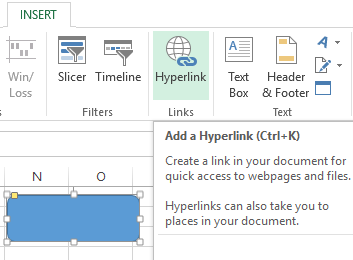
After clicking, a window will be opened. This window is intended for creating a connection between the button and a file, web page, e-mail, new document, and location in the current Excel document.

It is enough to choose the desired option and specify the path to it. This method doesn’t require writing macros and provides the user with a wide range of opportunities.

Similar tasks can be performed with the help of macros. For example, for a user to go to a certain cell (M6) when clicking the button, the following code should be written:

Sub Macro1()
Range(«M6»).Select
End Sub

Similarly, you can assign a macro to a chart, WordArt and SmartArt objects.

How to make the sort button for tables in Excel

For an illustrative example, create a test table as in the figure:

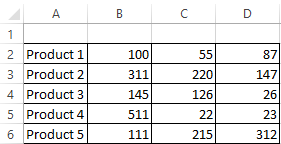
1. Instead of the table column headers, add shapes that will serve as buttons for sorting by the columns of the table.



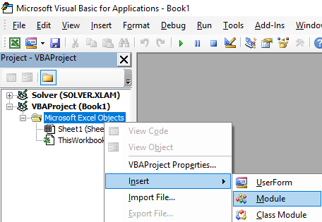
2. In the Visual Basic mode (ALT + F11), insert the new module (Module1) in the Modules folder. To do this, right-click on the folder and choose Insert-Module.



3. Double click on Module1 and enter the following code into it:
   

   
Sub Macro1()
    ActiveWorkbook.Worksheets("Sheet1").Sort.SortFields.Clear
    ActiveWorkbook.Worksheets("Sheet1").Sort.SortFields.Add Key:=Range("A2:A6"), _
        SortOn:=xlSortOnValues, Order:=xlAscending, DataOption:=xlSortNormal
    With ActiveWorkbook.Worksheets("Sheet1").Sort
        .SetRange Range("A2:D6")
        .Apply
    End With
End Sub
Sub Macro2()
    ActiveWorkbook.Worksheets("Sheet1").Sort.SortFields.Clear
    ActiveWorkbook.Worksheets("Sheet1").Sort.SortFields.Add Key:=Range("B2:B6"), _
        SortOn:=xlSortOnValues, Order:=xlDescending, DataOption:=xlSortNormal
    With ActiveWorkbook.Worksheets("Sheet1").Sort
        .SetRange Range("A2:D6")
        .Apply
    End With
End Sub
Sub Macro3()
    ActiveWorkbook.Worksheets("Sheet1").Sort.SortFields.Clear
    ActiveWorkbook.Worksheets("Sheet1").Sort.SortFields.Add Key:=Range("C2:C6"), _
        SortOn:=xlSortOnValues, Order:=xlDescending, DataOption:=xlSortNormal
    With ActiveWorkbook.Worksheets("Sheet1").Sort
        .SetRange Range("A2:D6")
        .Apply
    End With
End Sub
Sub Macro4()
    ActiveWorkbook.Worksheets("Sheet1").Sort.SortFields.Clear
    ActiveWorkbook.Worksheets("Sheet1").Sort.SortFields.Add Key:=Range("D2:D6"), _
        SortOn:=xlSortOnValues, Order:=xlDescending, DataOption:=xlSortNormal
    With ActiveWorkbook.Worksheets("Sheet1").Sort
        .SetRange Range("A2:D6")
        .Apply
    End With
End Sub


   Note. Red text indicates different parameters for each column.

4. Assign to each shape its own macro: Macro1 for «NAME» Macro2 for «May», and so on.

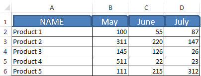
That’s all, now you just need to click on the header and the table will sort the data to a particular column. For convenience, Macro1 sorts the column «NAME» in ascending order due to Order:=xlAscending parameter. All other columns have assigned macros (2,3,4) with Order:=xlDescending parameter, which sets the sort type in descending order. This is done in order to show the user in which month more goods have been sold.

Download example of the sort button

Note. Such simple macros can be created in automatic mode without programming or without writing VBA (Visual Basic for Application) code, using the «Record Macro» tool.