
How to Make Boxes in Excel
- Open your spreadsheet.
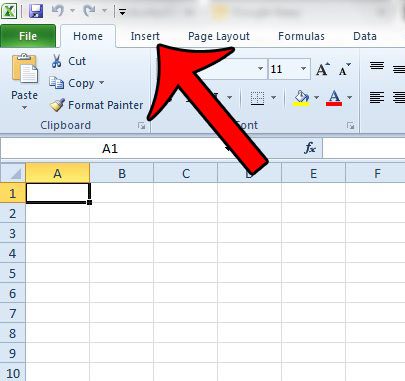
- Click Insert.
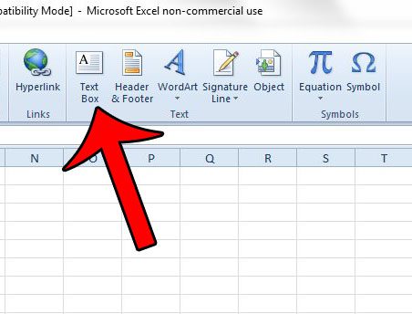
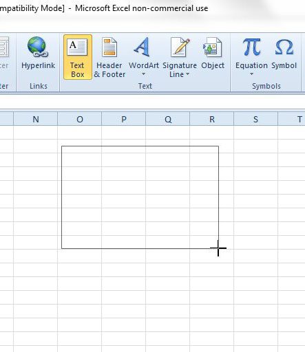
- Select the Text Box button.
- Draw the text box in the desired spot.
Contents
- 1 How do I make square boxes in Excel?
- 2 How do you use text boxes in Excel?
- 3 How do I add another box in Excel?
- 4 How do you make grid papers in Excel?
- 5 How do I make all the boxes the same size in Excel?
- 6 What are dashboards in Excel?
- 7 Where is the text box in Excel?
- 8 How do I create a multi column table in Excel?
- 9 How do you insert table style?
- 10 How do you make a paper grid?
- 11 How do I make rows and columns the same size in Excel?
- 12 How do I make all columns the same width in sheets?
- 13 How do I make a 100 chart on Excel?
- 14 What is grid in Excel?
- 15 How do I create a dashboard in Excel for beginners?
- 16 How do I create a dashboard?
- 17 How do you create a dashboard?
- 18 What is a floating text box?
- 19 Why do text boxes appear in Excel?
- 20 Where is the Developer tab in Excel?
How do I make square boxes in Excel?
Right-click the rectangle and choose Format AutoShape. Click the Size tab. In the Size And Rotate section, enter . 25″ for both the Height and Width to create a square.
How do you use text boxes in Excel?
- On the Insert tab, in the Text group, click Text Box.
- Click in the worksheet, and then drag to draw the text box the size that you want.
- To add text to a text box, click inside the text box, and then type or paste text. Notes: To format text in the text box, use the formatting options in the Font group on the Home tab.
How do I add another box in Excel?
Select the cell, or the range of cells, to the right or above where you want to insert additional cells. Tip: Select the same number of cells as you want to insert. For example, to insert five blank cells, select five cells. Hold down CONTROL, click the selected cells, then on the pop-up menu, click Insert.
How do you make grid papers in Excel?
To setup the grid
- Open a blank worksheet and Select All (Ctrl+A)
- Right mouse click on any Row number and choose Row Height.
- Type; 12 and click Ok.
- Right mouse click on any Column letter and choose Column Width.
- Type; 1.44 (20 pixels) and click OK.
- From the Page Layout ribbon, in the Page Setup group.
How do I make all the boxes the same size in Excel?
If you want to resize your entire worksheet, do the following:
- Click on the ‘Select All’ button on the top-left of the Excel window.
- Set the Column width for all the cells. Right-click on any column header.
- Set the Row height for all the cells. Right-click on any row, select ‘Row Height’ from the popup menu.
What are dashboards in Excel?
A dashboard is a visual representation of key metrics that allow you to quickly view and analyze your data in one place. Dashboards not only provide consolidated data views, but a self-service business intelligence opportunity, where users are able to filter the data to display just what’s important to them.
Where is the text box in Excel?
To insert a text box, click the Insert ribbon and click the Text Box icon on the far right. Then use the mouse to draw the text box above the sheet grid. To link a text box to a cell, have the text box selected, click in the Formula Bar and press = and then click the cell to link to and press Enter – see Figure 02.
How do I create a multi column table in Excel?
How to combine two or more columns in Excel
- In Excel, click the “Insert” tab in the top menu bar.
- In the “Create Table” dialog box that pops up, edit the formula so that only the columns and rows that you want to combine are used in the table.
How do you insert table style?
To apply a table style:
- Click anywhere in your table to select it, then click the Design tab on the far right of the Ribbon.
- Locate the Table Styles group, then click the More drop-down arrow to see the full list of styles.
- Select the table style you want.
- The table style will appear.
How do you make a paper grid?
Go to Ribbon > Design tab. Then, click the Page Color button and choose Fill Effects from the dropdown. Click the Pattern tab to display the design choices available to you. For example, to make a typical graph paper in Word, you can choose the Small grid or Large grid pattern.
How do I make rows and columns the same size in Excel?
How to make all rows and columns same size in Excel – Excelchat
- Step 1: Open the sheet with cells to resize. Double-click on the sheet to open it.
- Step 2: select the entire worksheet. The next thing to do is to select the whole worksheet.
- Step 3: Set all rows same size.
How do I make all columns the same width in sheets?
How to Set All Google Sheets Columns to the Same Width
- Open your spreadsheet.
- Click on the first column letter, hold down Shift, then click on the last column letter.
- Right click on a selected cell and choose Resize columns.
- Enter the column width and click OK.
How do I make a 100 chart on Excel?
Use the right arrow key on your keyboard to move to the right, into cell D2, and type the number 2 . Next, click into cell C3, just below the number 1 you typed, and type the number 11 . Move to the right one cell and type the number 12 . Excel will be used to put the other 96 numbers into your hundreds chart.
What is grid in Excel?
Gridlines in Excel are the horizontal and vertical gray lines that differentiate between cells in a worksheet.They also help users navigate through the worksheet columns and rows with ease.
How do I create a dashboard in Excel for beginners?
Here’s a step-by-step Excel dashboard tutorial:
- How to Bring Data into Excel. Before creating dashboards in Excel, you need to import the data into Excel.
- Set Up Your Excel Dashboard File.
- Create a Table with Raw Data.
- Analyze the Data.
- Build the Dashboard.
- Customize with Macros, Color, and More.
How do I create a dashboard?
Now we will focus on 10 essential tips and best practices to follow when creating dashboards, starting with defining your audience.
- Define Your Dashboard Audience And Objective.
- Make Sure Your Data Is Clean And Correct.
- Select The Right Chart Type For Your Data.
- Build a Balanced Perspective.
- Use Predefined Templates.
How do you create a dashboard?
How to design and build a great dashboard
- Be clear about what you’re trying to achieve.
- Include only the most important content.
- Use size and position to show hierarchy.
- Give your numbers context.
- Group your related metrics.
- Be consistent.
- Use clear labels your audience will understand.
- Round your numbers.
What is a floating text box?
Text boxes in Microsoft Word are graphic elements that contain editable text.If you specify a text box object to sit in front of the text on the page instead of in line, the box appears to float over the words.
Why do text boxes appear in Excel?
There’s a type of text box in an Excel file that is associated with a cell and appears only when you select that cell uniquely (e.g., by clicking on it or moving to it with cursor keys).
Where is the Developer tab in Excel?
The Developer tab isn’t displayed by default, but you can add it to the ribbon. On the File tab, go to Options > Customize Ribbon. Under Customize the Ribbon and under Main Tabs, select the Developer check box.
Excel for Microsoft 365 Excel 2021 Excel 2019 Excel 2016 Excel 2013 Excel 2010 Excel 2007 Excel Starter 2010 More…Less
When you want to display a list of values that users can choose from, add a list box to your worksheet.
Add a list box to a worksheet
-
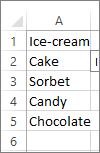
Create a list of items that you want to displayed in your list box like in this picture.

-
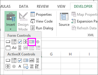
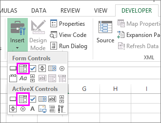
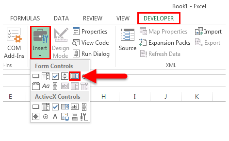
Click Developer > Insert.
Note: If the Developer tab isn’t visible, click File > Options > Customize Ribbon. In the Main Tabs list, check the Developer box, and then click OK.
-
Under Form Controls, click List box (Form Control).
-
Click the cell where you want to create the list box.
-
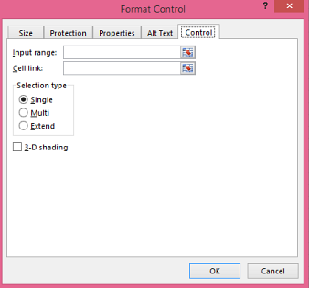
Click Properties > Control and set the required properties:
-
In the Input range box, type the range of cells containing the values list.
Note: If you want more items displayed in the list box, you can change the font size of text in the list.
-
In the Cell link box, type a cell reference.
Tip: The cell you choose will have a number associated with the item selected in your list box, and you can use that number in a formula to return the actual item from the input range.
-
Under Selection type, pick a Single and click OK.
Note: If you want to use Multi or Extend, consider using an ActiveX list box control.
-
Add a combo box to a worksheet
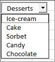
You can make data entry easier by letting users choose a value from a combo box. A combo box combines a text box with a list box to create a drop-down list.
You can add a Form Control or an ActiveX Control combo box. If you want to create a combo box that enables the user to edit the text in the text box, consider using the ActiveX Combo Box. The ActiveX Control combo box is more versatile because, you can change font properties to make the text easier to read on a zoomed worksheet and use programming to make it appear in cells that contain a data validation list.
-
Pick a column that you can hide on the worksheet and create a list by typing one value per cell.
Note: You can also create the list on another worksheet in the same workbook.
-
Click Developer > Insert.
Note: If the Developer tab isn’t visible, click File > Options > Customize Ribbon. In the Main Tabs list, check the Developer box, and then click OK.
-
Pick the type of combo box you want to add:
-
Under Form Controls, click Combo box (Form Control).
Or
-
Under ActiveX Controls, click Combo Box (ActiveX Control).
-
-
Click the cell where you want to add the combo box and drag to draw it.
Tips:
-
To resize the box, point to one of the resize handles, and drag the edge of the control until it reaches the height or width you want.
-
To move a combo box to another worksheet location, select the box and drag it to another location.
Format a Form Control combo box
-
Right-click the combo box and pick Format Control.
-
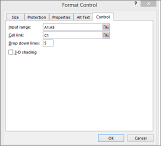
Click Control and set the following options:
-
Input range: Type the range of cells containing the list of items.
-
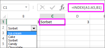
Cell link: The combo box can be linked to a cell where the item number is displayed when you select an item from the list. Type the cell number where you want the item number displayed.
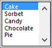
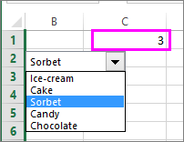
For example, cell C1 displays 3 when the item Sorbet is selected, because it’s the third item in our list.
Tip: You can use the INDEX function to show an item name instead of a number. In our example, the combo box is linked to cell B1 and the cell range for the list is A1:A2. If the following formula, is typed into cell C1: =INDEX(A1:A5,B1), when we select the item «Sorbet» is displayed in C1.
-
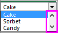
Drop-down lines: The number of lines you want displayed when the down arrow is clicked. For example, if your list has 10 items and you don’t want to scroll you can change the default number to 10. If you type a number that’s less than the number of items in your list, a scroll bar is displayed.
-
-
Click OK.
Format an ActiveX combo box
-
Click Developer > Design Mode.
-
Right-click the combo box and pick Properties, click Alphabetic, and change any property setting that you want.
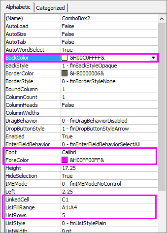
Here’s how to set properties for the combo box in this picture:
To set this property
Do this
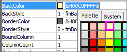
Fill color
Click BackColor > the down arrow > Pallet, and then pick a color.
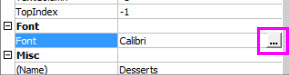
Font type, style or size
Click Font > the… button and pick font type, size, or style.
Font color
Click ForeColor > the down arrow > Pallet, and then pick a color.
Link a cell to display selected list value.
Click LinkedCell
Link Combo Box to a list
Click the box next to ListFillRange and type the cell range for the list.
Change the number of list items displayed
Click the ListRows box and type the number of items to be displayed.
-
Close the Property box and click Designer Mode.
-
After you complete the formatting, you can right-click the column that has the list and pick Hide.
Need more help?
You can always ask an expert in the Excel Tech Community or get support in the Answers community.
See Also
Overview of forms, Form controls, and ActiveX controls on a worksheet
Add a check box or option button (Form controls)
Need more help?
Want more options?
Explore subscription benefits, browse training courses, learn how to secure your device, and more.
Communities help you ask and answer questions, give feedback, and hear from experts with rich knowledge.
Adding text boxes in Microsoft Excel may seem odd, considering the layout of a spreadsheet and the way that the application is generally.
But you can definitely encounter situations where text boxes are a preferable choice for some data or information.
The ability to move the text box alone can make it appealing, and you can even have a linked cell in a text box so that you can display that data in the box.
Excel 2010’s system of cells provides for an efficient way to organize and manipulate your data.
But occasionally you may be using Excel for a purpose that requires certain data to be placed in a text box instead of a cell.
Text boxes are very versatile, and you can adjust both their appearance and location with just a few clicks of your mouse.
Our guide below will show you where to find the tool that inserts text boxes into your spreadsheet. We will also direct you to the assorted text box menus so that you can adjust your text box settings as needed.
- Open your spreadsheet.
- Click Insert.
- Select the Text Box button.
- Draw the text box in the desired spot.
Our article continues below with additional information on making a text box in Microsoft Excel 2010, including pictures of these steps.
If you are using Photoshop to edit your pictures, then you might be looking for a way to isolate edits to laters. Our adjust layer size Photoshop article can show you how to change the size of the objects on just one of your layers.
How to Insert a Text Box in Excel 2010 (Guide with Pictures)
These steps were written specifically for Microsoft Excel 2010. You can also insert text boxes in other versions of Microsoft Excel, although the exact steps may vary slightly from those presented here.
Step 1: Open your file in Microsoft Excel 2010.
Step 2: Click the Insert tab at the top of the window.
Step 3: Click the Text Box button in the Text section of the Office ribbon.
Step 4: Click and hold in the spot on your worksheet where you wish to insert the text box, then drag your mouse to adjust the size of the text box. Release the mouse button when you are ready to create the text box.
Note that you can adjust the size or the location of the text box later, if you wish.
Our article continues below with additional information on how to customize a text box in Excel.
How to Change the Appearance Text Boxes in Excel
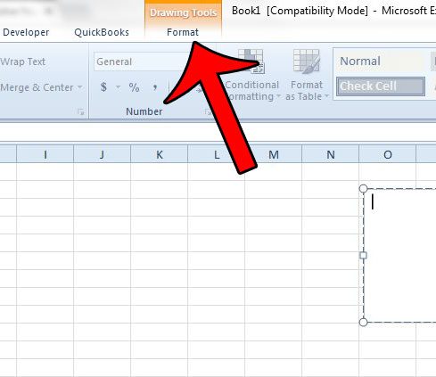
If you wish to adjust the appearance of the text box, you can click the Format tab at the top of the window, under Drawing Tools.
Additionally you can right-click inside of the text box, then select the Format Text Effects or Format Shape option for more settings.
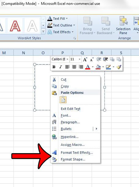
For example, you can remove the border from your text box if you wish to do so.
More Information on How to Make a Text Box in Excel 2010
- While a text box in Microsoft Excel may be used simply as a way to add content to your worksheet without actually placing it in the cells of that worksheet, it’s possible to have a linked cell that populates its data inside the text box. Simply click inside the text box, then click inside the formula bar and type =XX but replace the XX with the cell location. So, for example, if your data is inside cell A1, then you would type =A1.
- An Excel text box may be the focus of this article, but other Microsoft Office applications like Powerpoint and Word give you a way to add text to your document other than typing directly on the document page. You can add a text box in both of those applications if you click Insert at the top of the window and choose the Text Box option.
- You can resize your text box after creating it by clicking on one of the circular handles on the border of the text box. Note that this may adjust the layout of the information inside the text box depending on the manner in which you resize it.
Tips on Working with Text Boxes in Microsoft Excel
The text within a text box can be formatted in the same way that you format text in other documents. Simply type the text that you need, then select it and apply the desired formatting. Or you could make the formatting selection first, then type the text. This lets you do things like change a font, or a font color, or even a font size.
Knowing how to make boxes in Microsoft Excel can give you an extra tool when working with the application if you encounter a situation where the standard cell layout is insufficient. Whether you need to create a text box because you have a piece of information that isn’t part of a formula or won’t be included in any calculations, or you want to create an unusually sized object, a text box can be a helpful solution.
If you need to move to a new line in your text box, you can simply press Enter to do so. This works differently than forcing a new line inside of a standard Excel cell, as you need to hold down the Alt key and press Enter to add new lines within regular cells.
An Excel text box behaves in a similar manner to some other objects, like an image, in that it exists on a layer above the spreadsheet. This allows you to move the box freely around the worksheet. To move the text box, click inside of it, then click on the border and drag the box to a new location. Note that you can’t click on one of the control circles or the arrow, as that will resize the box.
Are you trying to use a formula in a text box, but are finding that the formula will not calculate a result? This article will show you how you can link a cell to a text box to achieve a result close to what you are looking for.

Matthew Burleigh has been writing tech tutorials since 2008. His writing has appeared on dozens of different websites and been read over 50 million times.
After receiving his Bachelor’s and Master’s degrees in Computer Science he spent several years working in IT management for small businesses. However, he now works full time writing content online and creating websites.
His main writing topics include iPhones, Microsoft Office, Google Apps, Android, and Photoshop, but he has also written about many other tech topics as well.
Read his full bio here.
I am sure you would have worked with the text boxes in Word or PowerPoint or even Excel but the trick I am going to share with you will make the text boxes dynamic.. in simple terms the text can change as per the situation
The applications of this technique in Dashboards, Charts and Visualizations is pretty helpful
Here is a standard Text Box in Excel..
- You’ll find the option to insert the text box in the Insert Tab
- Just draw the text box and start typing
But the problem is : If you write anything into it, it is a static text !
Here is how you can make it Dynamic..
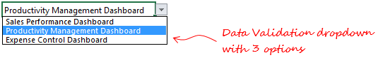
Step 1 : Insert a Data Validation Drop Down
Step 2 : Create a Text box and write anything into it
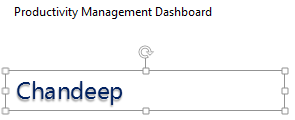 —> Wrote my name in the textbox
Step 3 : Link the text box to the cell value
- Select the text box
- Go to the formulas tab
- Write “=” and the cell address to which you want to link the cell, then press Enter
- Now when the value in the cell changes the text box will dynamically change
There are 2 things that you must remember about dynamic text boxes
- After typing the cell address in the formula bar you must press Enter key to enable the link
- Once the text box has been linked to the cell, you can no more type inside the text box. You have to either
- Break the linking to type anything or
- Continue working with the linked cell
Now let’s take a look at a few applications of Text Boxes
Application 1 : Create Dynamic Comments
Sometime ago I created a Dashboard on Company Cost Structure. I had put in a comment section in the dashboard with updated automatically as one would change the options in the Dashboard.
I have used formulas to generate dynamic comments and then linked them to the text boxes
Application 2 : Create Dynamic Chart Titles
All that I have done is linked the chart title (textbox) to a cell which is displaying dynamic headlines
Application 3 : Create Dynamic Data Labels
- There is just one pain point – Linking each data labels (text boxes) to the cells values one by one (unfortunately there is no shortcut for that)
- Now when values in the cells will change the data labels will also automatically update
Excel 2013 offers customizing the data labels, which can be picked up from a cell address.
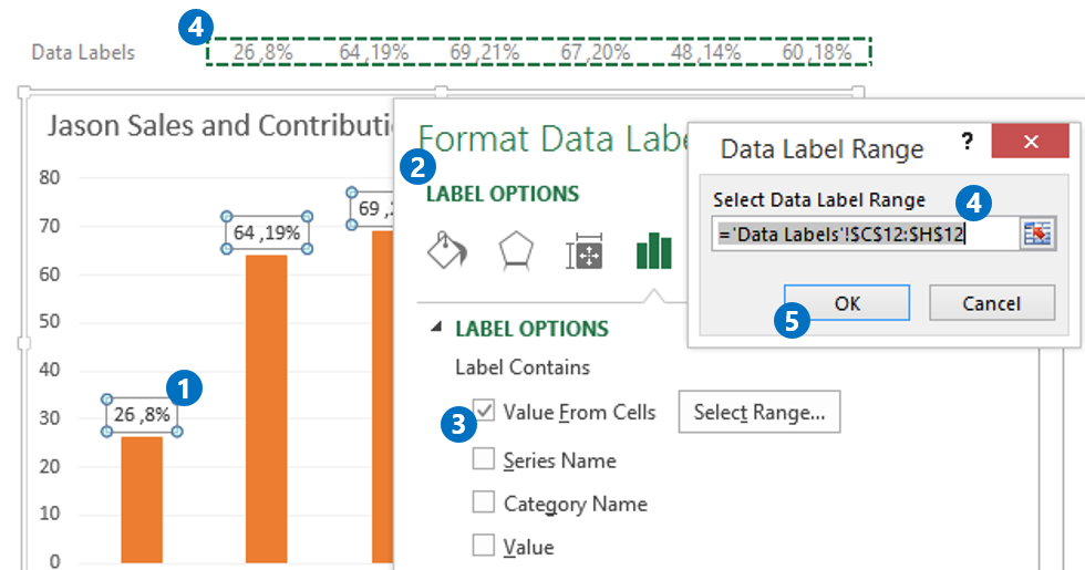
- Select the data labels
- Press Ctrl 1 to open Format Data Labels Box
- Click on Value from Cells
- Pick the values from the spreadsheet
- Click on Ok
Have you created a dynamic text box before ?
How do you use dynamic text boxes in work? If this is new to you share how do you think you’ll use it to make your report more dynamic?
More Resources on Creating Dynamic Objects
- Learn How Camera Tool Works in Excel – To make Pictures Dynamic
- How to Lookup Pictures – Picture VLOOKUP
- How to Filter Photos in Excel

Chandeep
Welcome to Goodly! My name is Chandeep.
On this blog I actively share my learning on practical use of Excel and Power BI. There is a ton of stuff that I have written in the last few years. I am sure you’ll like browsing around.
Please drop me a comment, in case you are interested in my training / consulting services. Thanks for being around
Chandeep
The list box in Excel (Table of Contents)
- List box in Excel
- How to Create List box in Excel?
- Examples of the List box in Excel
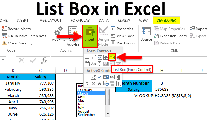
List Box in Excel
List Box in excel is used to create a list inside the box and choose them just we select the values from dropdown. List boxes are available in the Insert option in the Developer menu tab. We can use List boxes with VBA macro and also excel cells. Whatever values we select can be seen in the list box, and once we select any value that will be reflected, the cell linked to List Box.
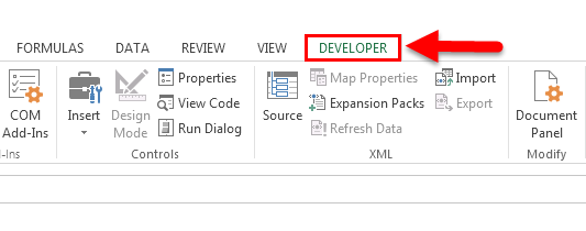
List Box is located under Developer Tab in Excel. If you are not a VBA macro user, you may not see this DEVELOPER tab in your excel.
Follow the below steps to unleash the Developer Tab.
If the Developer tab is not showing, then follow the below steps to enable the Developer tab.
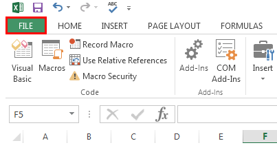
- Go to the FILE option (top of the left-hand side of the excel).
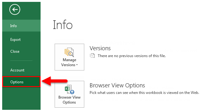
- Now go to Options.
- Go to Custom Ribbon and click on the Developer tab check-box.
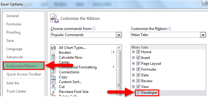
- Once the Developer Tab is enabled, you can see it on your excel ribbon.
How to Create List box in Excel?
Follow the below steps to insert the List box in excel.
You can download this List Box Excel Template here – List Box Excel Template
Step 1: Go to Developer Tab > Controls > Insert > Form Controls > List Box.
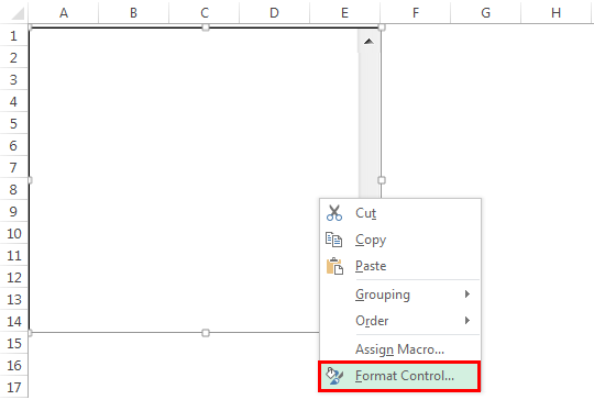
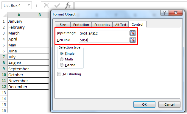
Step 2: Click on List Box and draw in the worksheet; then Right-click on the List Box and select the option Format Control.
Step 3: Create a month list in column A from A1 to A12.
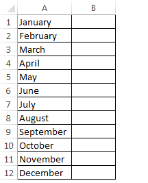
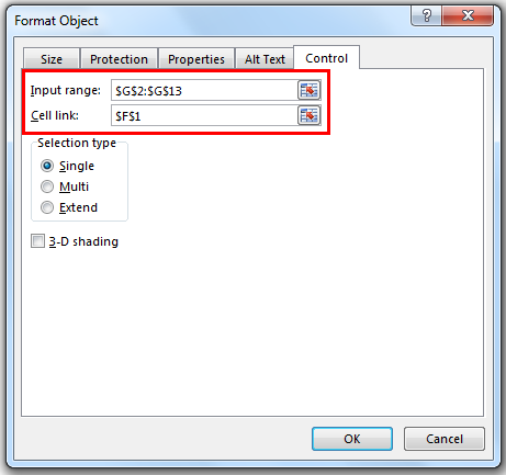
Step 4: Once you have selected Format Control, it will open the below dialog box; go to the Control tab in the input range select the month lists from A1 to A10. In the cell link, give a link to cell B1.
We have linked our cell to B1. Once the first value has selected the cell B1 will show 1. Similarly, if you select April, it will show 4 in cell B1.
Examples of List Box in Excel
Let’s look at a few examples of using Lise Box in Excel.
Example #1 – List Box with Vlookup Formula
Now we will look at the way of using List Box in excel.
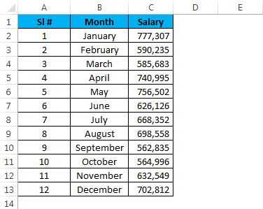
Assume you have salary data month-wise from A2 to A13. Based on the selection made from the list, it has to show the value for the selected month.
Step 1: Draw a List Box from the developer tab and create a list of months.
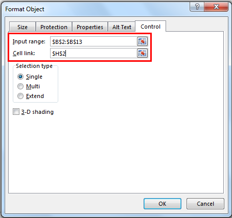
Step 2: I have given a cell link to H2. In G2 and G3, create a list like this.
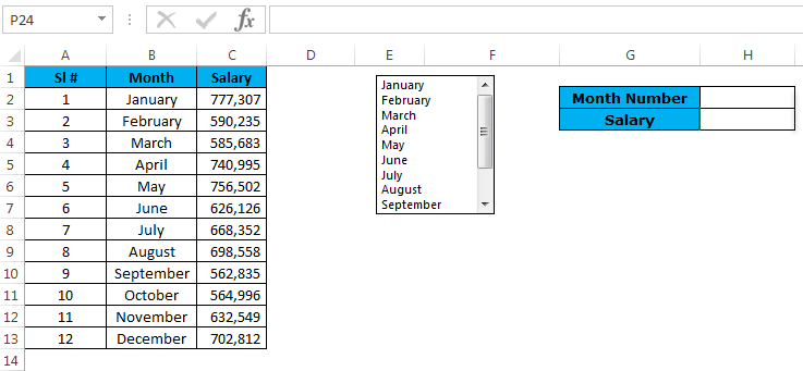
Step 3: Apply the VLOOKUP formula in cell H3 to get the salary data from the list.
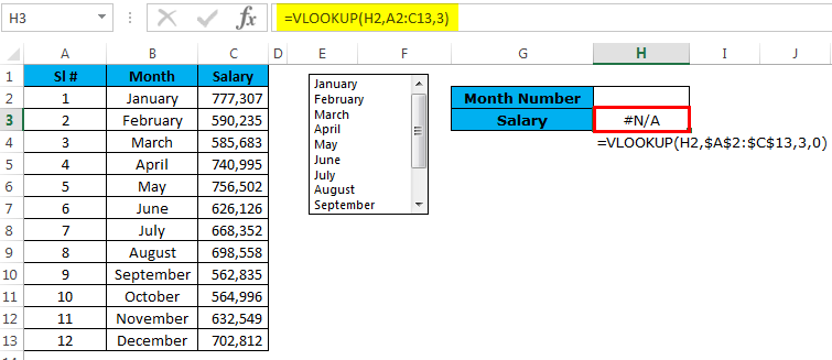
Step 4: Right now, it is showing an error as #N/A. Please select any of the months; it will show you the salary data for that month.
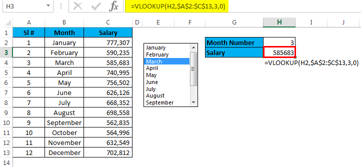
I have selected March month, and the number for March month is 3 and VLOOKUP showing the value for number 3 from the table.
Example #2 – Custom Chart with List Box
In this example, I will explain how to create the custom chart using List Box. I will take the same example that I have used previously.
Step 1: Create a table like this.
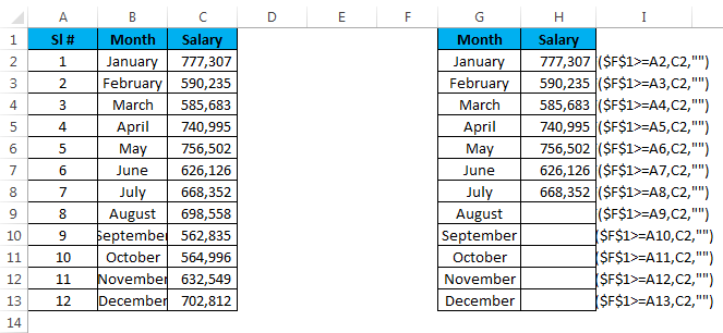
Step 2: Insert List Box from the Developer tab. Go to Format Control give a link to the month list and a cell link to F1.
Step 3: Apply the IF formula in the newly created table.
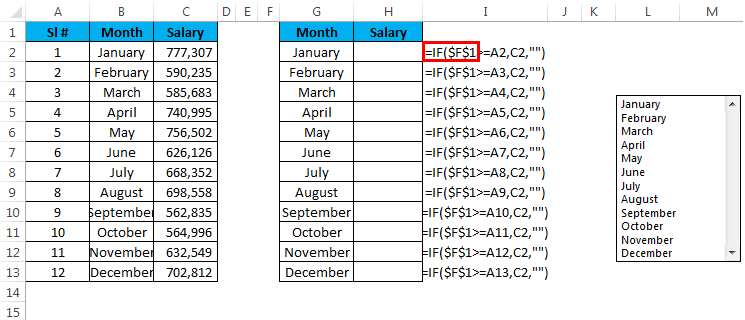
I have applied the IF condition to the table. If I select the month March, the value in cell F1 will show the number 3 because March is the third value in the list. Similarly, it will show 4 for April, 10 for October and 12 for December.
IF condition checks if the value in the cell F1 is greater than equal to 4, it will show for the value for the first 4 months. If the value in cell F1 is greater than equal to 6, it will show the value for the first 6 months only.
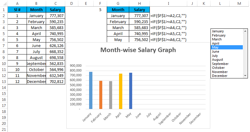
Step 4: Now apply the chart for the modified table with the IF condition.
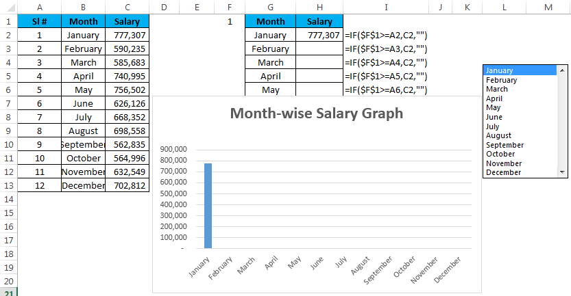
Step 5: Now it is showing the empty graph. Select the month to see the magic. I have selected the month of May, which is why it shows the graph for the first 5 months.
Things to Remember
- There is one more List Box under Active X Control in excel. This has mainly used in VBA macros.
- Cell link is to indicate which item from the list has selected.
- We can control the user to enter the data by using List Box.
- We can avoid wrong data entry by using List Box.
Recommended Articles
This has been a guide to the List box in Excel. Here we discuss the List box in Excel and How to create the List box in Excel along with practical examples and a downloadable excel template. You can also go through our other suggested articles –
- Name Box in Excel
- Excel Search Box
- CheckBox in Excel
- Compare Two Lists in Excel