
-
Select a cell within your data.
-
Select Home > Format as Table.
-
Choose a style for your table.
-
In the Create Table dialog box, set your cell range.
-
Mark if your table has headers.
-
Select OK.
-
Insert a table in your spreadsheet. See Overview of Excel tables for more information.
-
Select a cell within your data.
-
Select Home > Format as Table.
-
Choose a style for your table.
-
In the Create Table dialog box, set your cell range.
-
Mark if your table has headers.
-
Select OK.
To add a blank table, select the cells you want included in the table and click Insert > Table.
To format existing data as a table by using the default table style, do this:
-
Select the cells containing the data.
-
Click Home > Table > Format as Table.
-
If you don’t check the My table has headers box, Excel for the web adds headers with default names like Column1 and Column2 above the data. To rename a default header, double-click it and type a new name.
Note: You can’t change the default table formatting in Excel for the web.
Formatting cells as a table this is a process, that requires a lot of time, but that brings little benefit. A lot of effort can be saved by using ready-made styles of table layout.
Let`s descry ready-made designer stylish solutions that are predefined in the Excel tool set. You can also think about creating and maintaining your own styles. For this purpose, the program provides for special tools and tools.
How to create and format as a table in Excel?
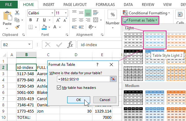
We format the original range from the previous lessons with the helping of style design.
- Move the cursor to any cell in the table within the range A1:D4.
- Select the «Format as Table» tool on the «HOME» tab, the «Styles» section. There are the wide selection of ready-made and harmonious in design styles before you . Specify the style «Style Light 2». The dialog box appears where the range of the table data location is determined. Do not change anything, pressing OK.
- The table has completely changed into a new and stylish format. There are even added filter control buttons. And on the broad band of tools the bookmark «DESIGN» was added, above which the inscription «TABLES TOOLS» is highlighted.
- To remove all unnecessary from our table and leave only the format, go to the «Designer» tab and in the «Tools» section, select «Convert to Range». Press OK to confirm.
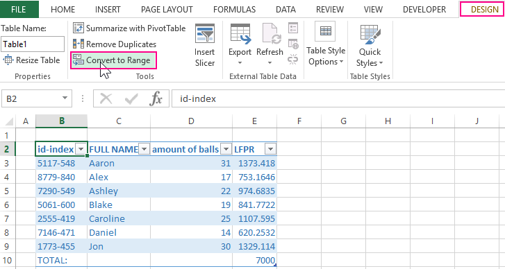
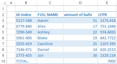
The notation. Note, that Excel itself recognized to the size of the table, we did not need to allocate a range, it was enough to specify one of any cells.
Although there are a lot of styles, sometimes you can not find the right one. To save time, you should choose the most similar style and format it for your needs.
To clear the format, you must first select the required range of cells and select the tool on the «HOME tab» – «Editing» – «Clear Formats». For quick removal only of the cell boundaries, use the shortcut key combination CTRL + SHIFT + (minus). Just do not forget to select the range before that.
Convert Data Into a Table in Excel
This page will show you how to convert Excel data into a table.
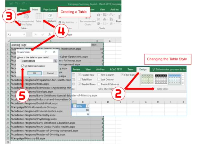
Creating a Table within Excel
- Open the Excel spreadsheet.
- Use your mouse to select the cells that contain the information for the table.
- Click the «Insert» tab > Locate the «Tables» group.
- Click «Table». A «Create Table» dialog box will open.
- If you have column headings, check the box «My table has headers».
- Verify that the range is correct > Click [OK].
- Resize your columns to make the headings visible.
Changing the Table Style
- Click on a cell in the table to activate the «Table Tools» tab.
- Click the «Design» tab > Locate the «Table Styles» group.
- Choose a style/color option that appeals to you. (Hover over the various table styles to see a live preview.)
Keywords: Office, color, colors, filter, sort, rows, columns, apply, enhance, table
Share This Post
-
Facebook
-
Twitter
-
LinkedIn
Blog Resources
Cedarville offers more than 150 academic programs to grad, undergrad, and online students. Cedarville is known for its biblical worldview, academic excellence, intentional discipleship, and authentic Christian community.

Loading…
Содержание
- Основы создания таблиц в Excel
- Способ 1: Оформление границ
- Способ 2: Вставка готовой таблицы
- Способ 3: Готовые шаблоны
- Вопросы и ответы

Обработка таблиц – основная задача Microsoft Excel. Умение создавать таблицы является фундаментальной основой работы в этом приложении. Поэтому без овладения данного навыка невозможно дальнейшее продвижение в обучении работе в программе. Давайте выясним, как создать таблицу в Экселе.
Таблица в Microsoft Excel это не что иное, как набор диапазонов данных. Самую большую роль при её создании занимает оформление, результатом которого будет корректное восприятие обработанной информации. Для этого в программе предусмотрены встроенные функции либо же можно выбрать путь ручного оформления, опираясь лишь на собственный опыт подачи. Существует несколько видов таблиц, различающихся по цели их использования.
Способ 1: Оформление границ
Открыв впервые программу, можно увидеть чуть заметные линии, разделяющие потенциальные диапазоны. Это позиции, в которые в будущем можно занести конкретные данные и обвести их в таблицу. Чтобы выделить введённую информацию, можно воспользоваться зарисовкой границ этих самых диапазонов. На выбор представлены самые разные варианты чертежей — отдельные боковые, нижние или верхние линии, толстые и тонкие и другие — всё для того, чтобы отделить приоритетную информацию от обычной.
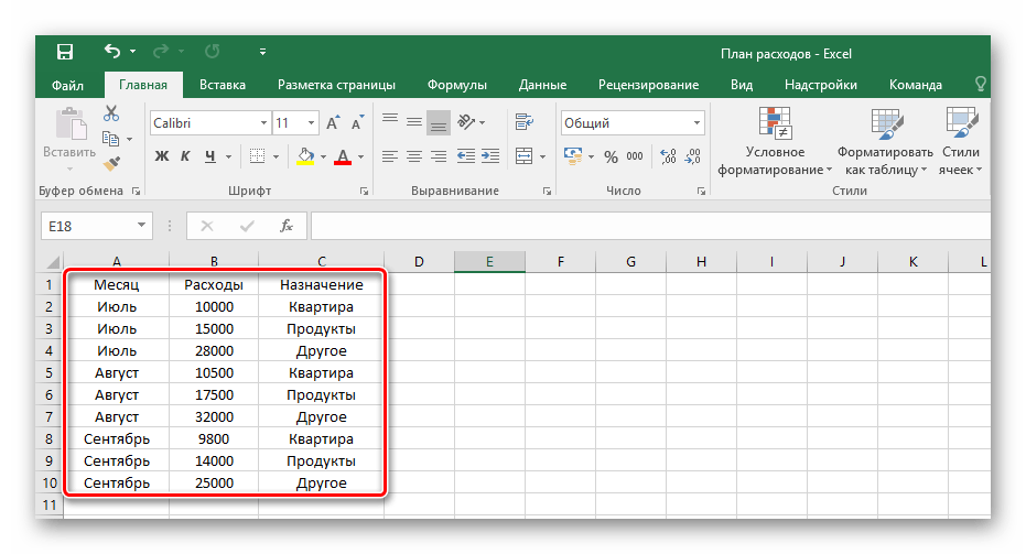
- Для начала создайте документ Excel, откройте его и введите в желаемые клетки данные.
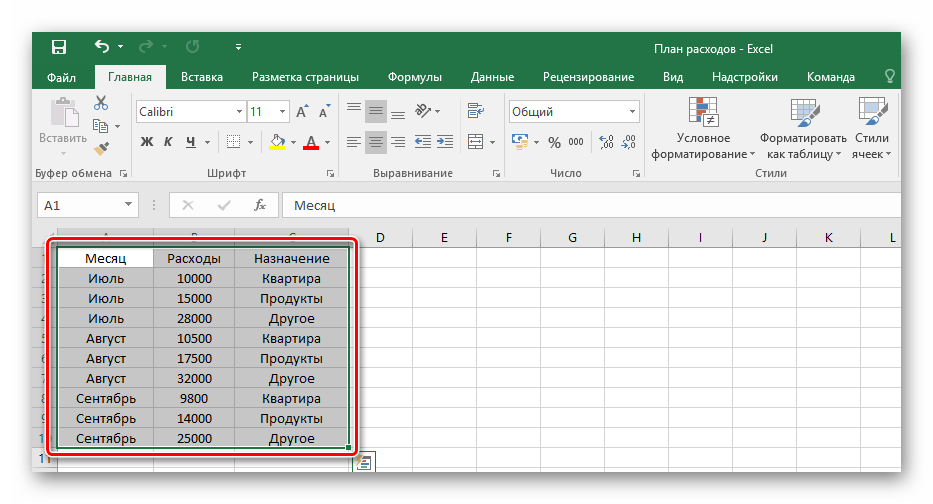
- Произведите выделение ранее вписанной информации, зажав левой кнопкой мыши по всем клеткам диапазона.
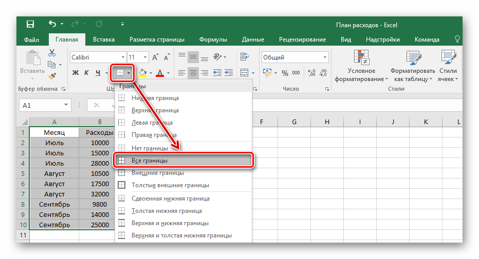
- На вкладке «Главная» в блоке «Шрифт» нажмите на указанную в примере иконку и выберите пункт «Все границы».
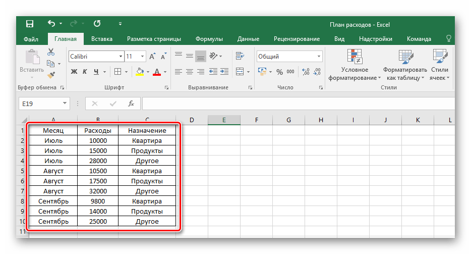
- В результате получится обрамленный со всех сторон одинаковыми линиями диапазон данных. Такую таблицу будет видно при печати.
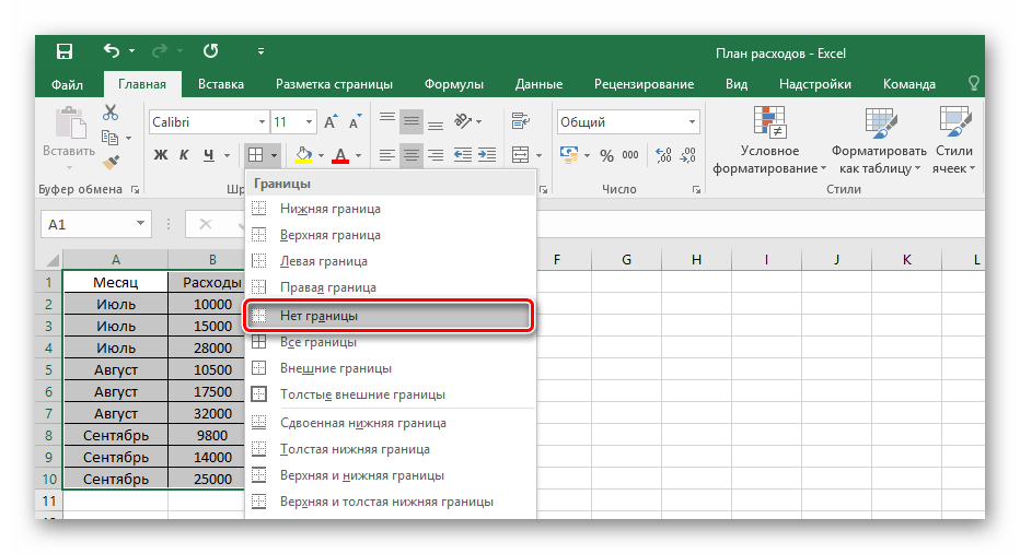
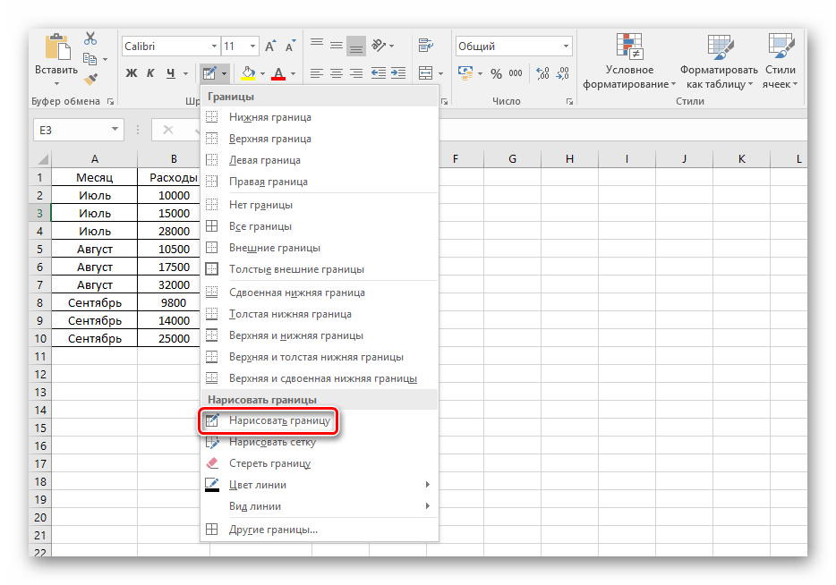
- Для ручного оформления границ каждой из позиций можно воспользоваться специальным инструментом и нарисовать их самостоятельно. Перейдите уже в знакомое меню выбора оформления клеток и выберите пункт «Нарисовать границу».
Соответственно, чтобы убрать оформление границ у таблицы, необходимо кликнуть на ту же иконку, но выбрать пункт «Нет границы».
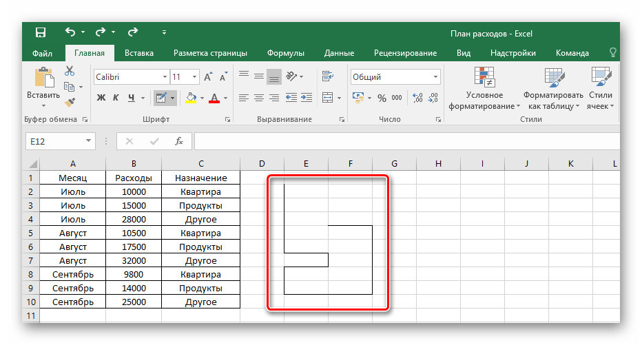
Пользуясь выбранным инструментом, можно в произвольной форме разукрасить границы клеток с данными и не только.
Обратите внимание! Оформление границ клеток работает как с пустыми ячейками, так и с заполненными. Заполнять их после обведения или до — это индивидуальное решение каждого, всё зависит от удобства использования потенциальной таблицей.
Способ 2: Вставка готовой таблицы
Разработчиками Microsoft Excel предусмотрен инструмент для добавления готовой шаблонной таблицы с заголовками, оформленным фоном, границами и так далее. В базовый комплект входит даже фильтр на каждый столбец, и это очень полезно тем, кто пока не знаком с такими функциями и не знает как их применять на практике.

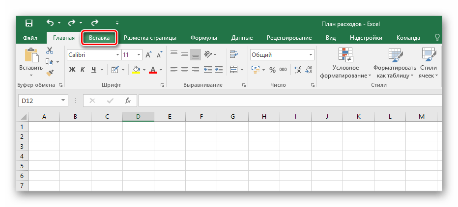
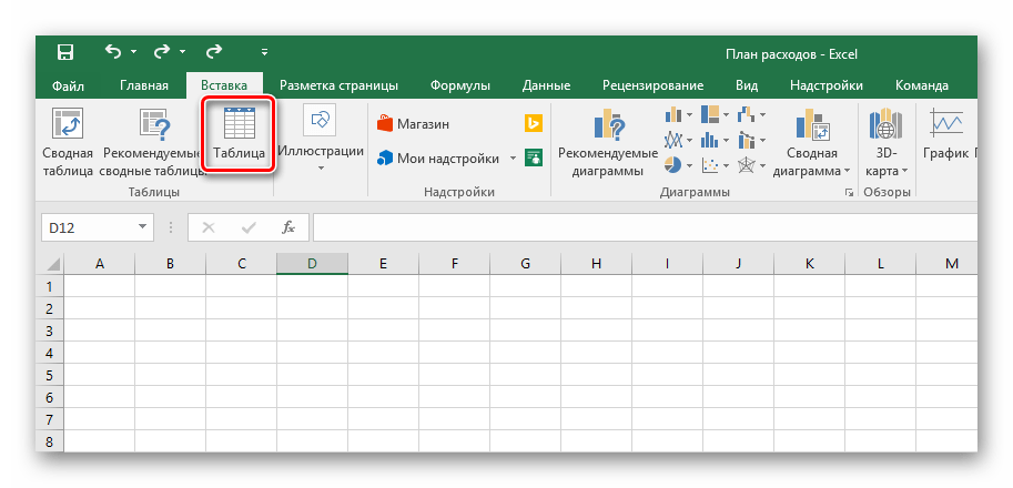
- Переходим во вкладку «Вставить».
- Среди предложенных кнопок выбираем «Таблица».
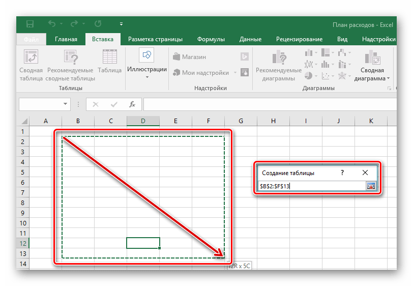
- После появившегося окна с диапазоном значений выбираем на пустом поле место для нашей будущей таблицы, зажав левой кнопкой и протянув по выбранному месту.
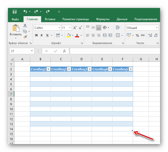
- Отпускаем кнопку мыши, подтверждаем выбор соответствующей кнопкой и любуемся совершенно новой таблице от Excel.
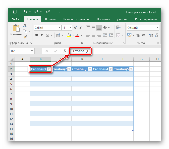
- Редактирование названий заголовков столбцов происходит путём нажатия на них, а после — изменения значения в указанной строке.
- Размер таблицы можно в любой момент поменять, зажав соответствующий ползунок в правом нижнем углу, потянув его по высоте или ширине.
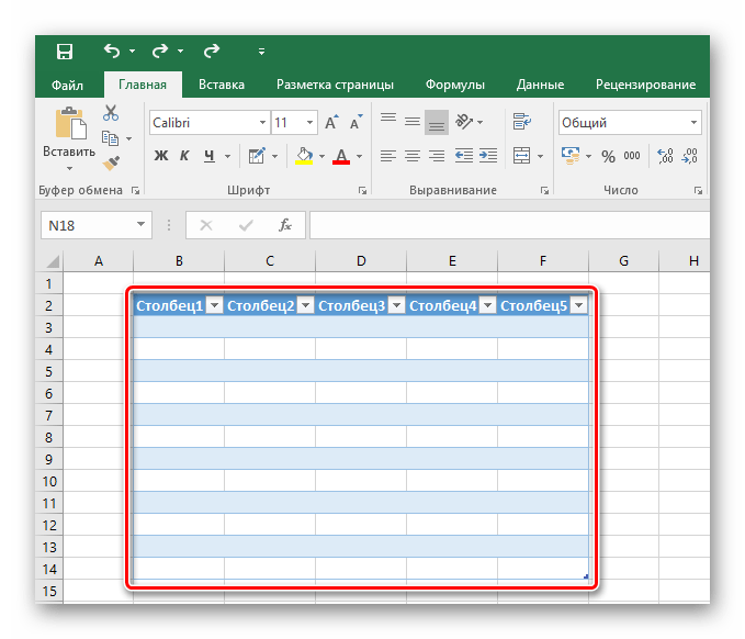
Таким образом, имеется таблица, предназначенная для ввода информации с последующей возможностью её фильтрации и сортировки. Базовое оформление помогает разобрать большое количество данных благодаря разным цветовым контрастам строк. Этим же способом можно оформить уже имеющийся диапазон данных, сделав всё так же, но выделяя при этом не пустое поле для таблицы, а заполненные клетки.
Способ 3: Готовые шаблоны
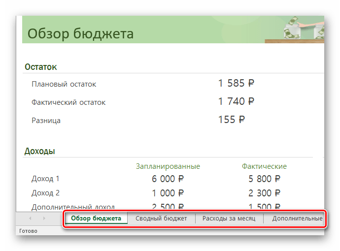
Большой спектр возможностей для ведения информации открывается в разработанных ранее шаблонах таблиц Excel. В новых версиях программы достаточное количество готовых решений для ваших задач, таких как планирование и ведение семейного бюджета, различных подсчётов и контроля разнообразной информации. В этом методе всё просто — необходимо лишь воспользоваться шаблоном, разобраться в нём и пользоваться в удовольствие.
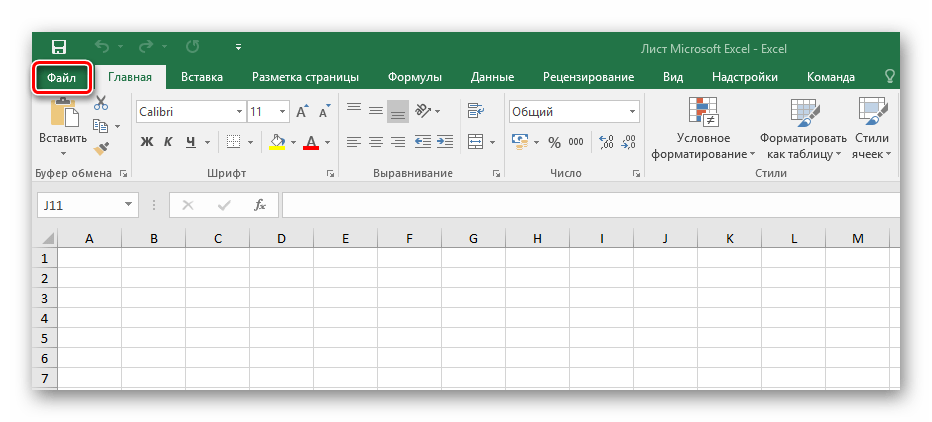
- Открыв Excel, перейдите в главное меню нажатием кнопки «Файл».
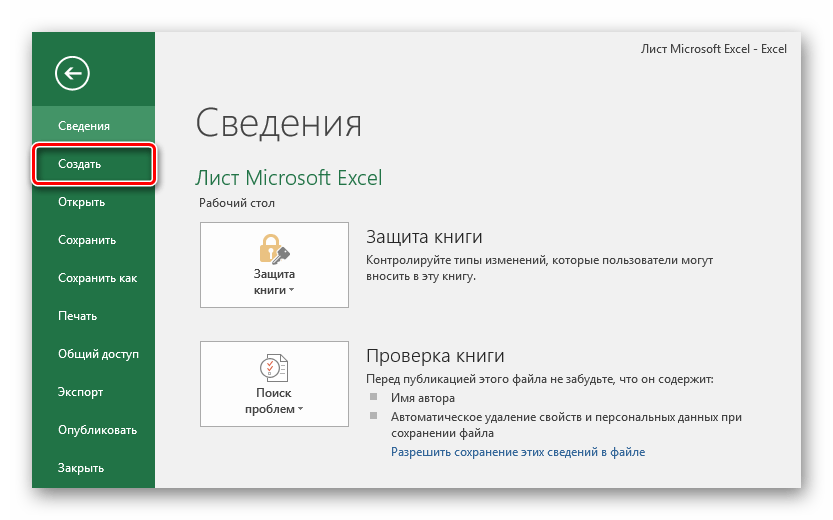
- Нажмите вкладку «Создать».
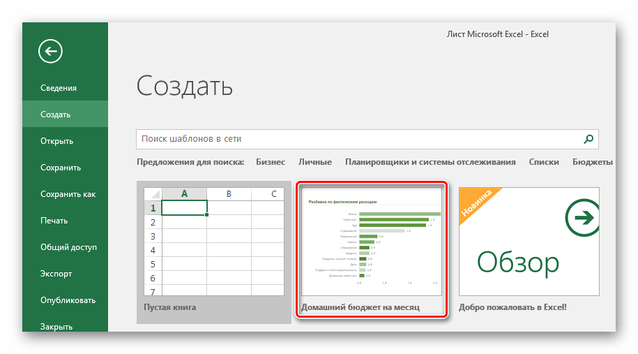
- Выберите любой понравившийся из представленных шаблон.
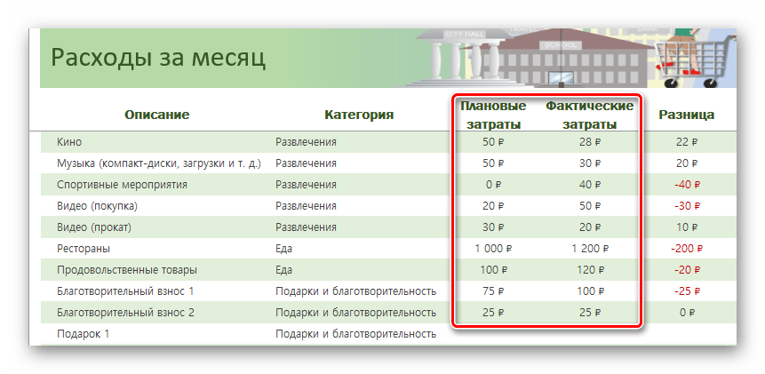
- Ознакомьтесь с вкладками готового примера. В зависимости от цели таблицы их может быть разное количество.
- В примере с таблицей по ведению бюджета есть колонки, в которые можно и нужно вводить свои данные — воспользуйтесь этим.
Таблицы в Excel можно создать как вручную, так и в автоматическом режиме с использованием заранее подготовленных шаблонов. Если вы принципиально хотите сделать свою таблицу с нуля, следует глубже изучить функциональность и заниматься реализацией таблицы по маленьким частицам. Тем, у кого нет времени, могут упростить задачу и вбивать данные уже в готовые варианты таблиц, если таковы подойдут по предназначению. В любом случае, с задачей сможет справиться даже рядовой пользователь, имея в запасе лишь желание создать что-то практичное.
Еще статьи по данной теме:
Помогла ли Вам статья?
Do you want to make a table in Excel? This post is going to show you how to create a table from your Excel data.
Entering and storing data is a common task in Excel. If this is something you’re doing, then you need to use a table.
Tables are containers for your data! They help you keep all your related data together and organized.
Tables have a lot of great features and work well with other tools inside and outside of Excel, so you should definitely be using them with your data.
This post is going to show you all the ways you can create a table from your data in Excel. Get your copy of the example workbook used in this post and follow along!
Tabular Data Format for Excel Tables
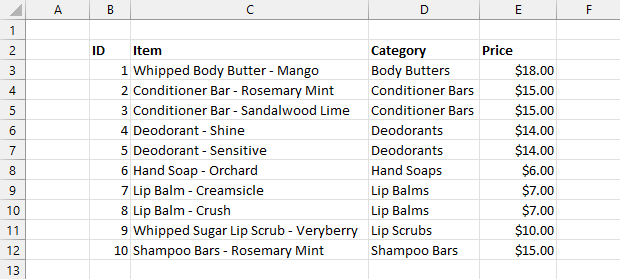
Excel tables are the perfect container for tabular datasets due to their row and column structure. Just make sure your data follows these rules.
- The first row of your dataset should contain a descriptive column heading.
- Your data should have no blank column headings.
- Your data should have no blank columns or blank rows.
- Your data should have no subtotals or grand totals.
- One row in your data should represent exactly one record of data.
- One column should contain exactly one type of data.
If your data is rectangular in shape and adheres to the above rules, then it’s ready to be put into a table.
Create a Table from the Insert Tab
Now that your data is ready to be placed inside a table, how can you do that?
It’s very easy and will only take a few clicks!
You’ll be able to add your data in a table from the Insert tab. Follow these steps to get your data into a table!
- Select a cell inside your data.
- Go to the Insert tab.
- Select the Table command in the Tables section.
This is going to open the Create Table menu with your data range selected. You should see a green dash line around your selected data and you can adjust the selection if needed.
- Check the My table has headers option. This is needed if the first row of your data contains column name headings.
- Press the OK button.
Your data is now inside a table! You’ll easily be able to tell the data is inside an Excel Table now because a default table formatting is automatically applied.
You can go to the Table Design tab and select other style options from the Table Styles section.
💡 Tip: Your table will get a default name such as Table1. You should give your new table a descriptive name as this is how you will refer to it in formulas and other tools.
Create a Table from the Home Tab
Another place you can access the table command is from the Home tab.
You can use the Format as Table command to create a table.
- Select a cell inside your data.
- Go to the Home tab.
- Select the Format as Table command in the Styles section.
- Select a style option for your table.
- Check the option for My table has headers.
- Press the OK button.
This is a great option as you get to choose the table style during the process of making your table.
Create a Table with a Keyboard Shortcut
Creating a table is such a common task that there is a keyboard shortcut for it.
Select your data and press Ctrl + T on your keyboard to turn your dataset into a table.
This is an easy shortcut to remember since T stands for Table.
There is also a legacy shortcut available from when tables were called lists. Select your data and if you press Ctrl + L this will also make a table. In this case, L stands for List.
Create a Table with Quick Analysis
When you select any range Excel will show you the Quick Analysis options in the lower right corner.
This will give you quick access to conditional formatting, pivot tables, charts, totals, and sparklines. The menu also includes the table command to convert the data into a table.
You can follow these steps to create a table from the Quick Analysis tools.
- Select your entire dataset. You can select any cell in the data and press Ctrl + A and this will select the full range.
This should automatically show the Quick Analysis tool in the lower right corner of the selected range.
- Click on the Quick Analysis tools or press Ctrl + Q to open the Quick Analysis menu.
- Go to the Tables tab.
- Click on the Table command. When you hover your cursor over the Table command it will show you a preview of your data inside a table!
📝 Note: This method allows you to skip the Create Table menu and the Quick Analysis will guess if your data has column headings or not. Excel will apply any column headings to your table accordingly.
Quick Analysis can be disabled from the Excel Options menu if the pop-up command is something you find annoying.
- Go to the File tab.
- Select the Options menu.
- Go to the General tab of the Excel Options menu.
- Uncheck the Show Quick Analysis options on selection option.
- Press the OK button.
📝 Note: This will only disable the small pop-up command from showing when you select your data. You can still use the Ctrl + Q keyboard shortcut to access the Quick Analysis tools for any selected range.
Create a Table with Power Query
Power Query is a very useful tool for transforming your data, but you can also create a table during the process of building your queries.
If your data isn’t already inside a table, you can use the From Table/Range query to make a table.
- Select your data.
- Go to the Data tab.
- Press the From Table/Range command in the Get & Transform Data section.
This will open the Create Table menu.
- Check the My table has headers option if the first row in your data contains column headings.
- Press the OK button.
This will add your data to a table and then open the Power Query Editor where you will be able to build your query based on the new table.
When you are finished building your query, you can go to the Home tab of the Power Query editor and press the Close and Load command.
This will give you the option to create another table filled with the transformed data. Select the Table option and press the OK button to load the transformed data into a table.
⚠️ Warning: This method does create a table, but doesn’t give you the opportunity to name the table before you build your queries. This means your queries will reference the generic table name such as Table1, and if you later change the table name you will also have to update the reference in your query.
Create Multiple Tables from a List with VBA
Suppose you need to create multiple tables in your Excel file. Maybe you need to create a table of sales data for each month of the year. Doing this manually could be a time-consuming process.
This is where you could use VBA to create multiple tables with the required columns.
Go to the Developer tab and select the Visual Basic command to open the visual basic editor. Then go to the Insert tab of the visual basic editor and select the Module option to create a new module to add your VBA macro.
Sub AddTables()
Dim myRange As Range
Dim sheetTest As Boolean
Dim myHeadings As Variant
Dim colCount As Integer
Set myRange = Selection

myHeadings = [{"ID","Date","Item","Quantity","Price"}]
colCount = UBound(myHeadings)

For Each c In myRange.Cells
sheetTest = False
    For Each ws In ThisWorkbook.Worksheets
        If ws.Name = c.Value Or c.Value = "" Then
            sheetTest = True
        End If
    Next ws
    If Not (sheetTest) Then
        With Sheets
            Sheets.Add.Name = c.Value
            Sheets(c.Value).Select
            Range("A1").Resize(1, colCount).Value = myHeadings
            ActiveSheet.ListObjects.Add(xlSrcRange, Range("A1").Resize(1, colCount), , xlYes).Name = c.Value & "Sales"
        End With
    End If
Next c
End Sub
This code will loop through the selected range and add a new sheet for each cell in the range. The code tests if the sheet name exists and if it doesn’t then it creates a new sheet named from the cell value.
The column headings are added to the new sheet starting at cell A1. This is then turned into a table and the table is named based on the sheet name.
myHeadings = [{"ID","Date","Item","Quantity","Price"}]The above line of code is used to create the column headings in each table. You can adjust this to suit your needs.
You can then run this macro to create multiple tables.
- Select the range of cells that contain the list the names for each table you want to create. For example, you might want a list of month names to create a table for each month.
- Press the Alt + F8 keyboard shortcut to open the Macro menu.
- Select your macro.
- Press the Run button.
This will run and create a new sheet for each item in your selection. Each sheet will contain a table with the same column headings and be named based on the items in the selected list.
Create Multiple Tables from a List with Office Scripts
If you are using Excel online and want to automate the process of creating multiple tables from a list, then you will need to use Office Scripts.
This is a JavaScript based language that can help you automate tasks in Excel online.
Go to the Automate tab and select the New Script command to open the Office Script Editor.
function main(workbook: ExcelScript.Workbook) {

	//Create an array with the column headings
	let myHeaders = [["ID", "Date", "Item", "Quantity", "Price"]]
	let colCount = myHeaders[0].length;
	//Create an array with the values from the selected range
	let selectedRange = workbook.getSelectedRange();
	let selectedValues = selectedRange.getValues();
	//Get dimensions of selected range
	let rowHeight = selectedRange.getRowCount();
	let colWidth = selectedRange.getColumnCount();

	//Loop through each item in the selected range
	for (let i = 0; i < rowHeight; i++) {
		for (let j = 0; j < colWidth; j++) {
			try {
				//Create a new sheet with name from the selected range
				let thisSheet = workbook.addWorksheet(selectedValues[i][j]);
				//Add column headings to new sheet and convert to table
				thisSheet.getRange("A1").getAbsoluteResizedRange(1, colCount).setValues(myHeaders);
				let newTable = workbook.addTable(thisSheet.getRange("A1").getAbsoluteResizedRange(1, colCount), true);
				newTable.setName(selectedValues[i][j] + "Sales");
			}
			catch (e) {
				//do nothing
			};
		};
	};
};
Copy and paste the above code into the Code Editor. Press the Save script button to save the script and then you can use the Run button to execute the script.
This Office Script code will loop through the active range in your workbook and create a new sheet for each cell in the selected range and name it based on the value in the cell.
let myHeaders = [["ID", "Date", "Item", "Quantity", "Price"]]The column headings are added to each new sheet starting in cell A1. You can adjust the above line of code to change the column headings to suit your needs.
These column headings are then turned into a table and the table is named based on the sheet name.
You can then run this script using the following steps.
- Select a range of cells that contain the list of tables you want to create.
- Click on the Run button in the Code Editor.
The code will run and create all the sheets with tables in each sheet.
Conclusions
Tables are a very useful feature for your tabular data in Excel.
Your data can be added to a table in several ways such as from the Insert tab, from the Home tab, with a keyboard shortcut, or using the Quick Analysis tools.
Tables work well with other tools in Excel such as Power Query. Because of this, Excel will even automatically convert your data into a table before using Power Query.
Creating multiple tables in your workbook can also be automated using either VBA or Office Scripts.
How do you make your tables? Do you know any other tips? Let me know in the comments section below!
About the Author
John is a Microsoft MVP and qualified actuary with over 15 years of experience. He has worked in a variety of industries, including insurance, ad tech, and most recently Power Platform consulting. He is a keen problem solver and has a passion for using technology to make businesses more efficient.