
Полезные макросы Excel для автоматизации рутинной работы с примерами применения для разных задач.
Примеры макросов для автоматизации работы
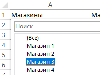 Макросы для фильтра сводной таблицы в Excel.
Как автоматизировать фильтр в сводных таблицах с помощью макроса? Исходные коды макросов для фильтрации и скрытия столбцов в сводной таблице.
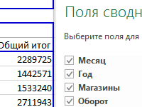 Макрос для создания сводной таблицы в Excel.
Как автоматически сгенерировать сводную таблицу с помощью макроса? Исходный код VBA для создания и настройки сводных таблиц на основе исходных данных.
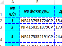 Макросы для изменения формата ячеек в таблице Excel.
Как форматировать ячейки таблицы макросом? Изменение цвета шрифта, заливки и линий границ, выравнивание. Автоматическая настройка ширины столбцов и высоты строк по содержимому с помощью VBA-макроса.
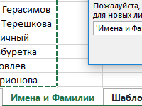 Макрос для копирования и переименования листов Excel.
Как одновременно копировать и переименовывать большое количество листов одним кликом мышкой? Исходный код макроса, который умеет одновременно скопировать и переименовать любое количество листов.
Using Excel Macros can speed up work and save you a lot of time.
One way of getting the VBA code is to record the macro and take the code it generates. However, that code by macro recorder is often full of code that is not really needed. Also macro recorder has some limitations.
So it pays to have a collection of useful VBA macro codes that you can have in your back pocket and use it when needed.
While writing an Excel VBA macro code may take some time initially, once it’s done, you can keep it available as a reference and use it whenever you need it next.
In this massive article, I am going to list some useful Excel macro examples that I need often and keep stashed away in my private vault.
I will keep updating this tutorial with more macro examples. If you think something should be on the list, just leave a comment.
You can bookmark this page for future reference.
Now before I get into the Macro Example and give you the VBA code, let me first show you how to use these example codes.
Using the Code from Excel Macro Examples
Here are the steps you need to follow to use the code from any of the examples:
- Open the Workbook in which you want to use the macro.
- Hold the ALT key and press F11. This opens the VB Editor.
- Right-click on any of the objects in the project explorer.
- Go to Insert –> Module.
- Copy and Paste the code in the Module Code Window.
In case the example says that you need to paste the code in the worksheet code window, double click on the worksheet object and copy paste the code in the code window.
Once you have inserted the code in a workbook, you need to save it with a .XLSM or .XLS extension.
How to Run the Macro
Once you have copied the code in the VB Editor, here are the steps to run the macro:
- Go to the Developer tab.
- Click on Macros.

- In the Macro dialog box, select the macro you want to run.
- Click on Run button.

In case you can’t find the developer tab in the ribbon, read this tutorial to learn how to get it.
Related Tutorial: Different ways to run a macro in Excel.
In case the code is pasted in the worksheet code window, you don’t need to worry about running the code. It will automatically run when the specified action occurs.
Now, let’s get into the useful macro examples that can help you automate work and save time.
Note: You will find many instances of an apostrophe (‘) followed by a line or two. These are comments that are ignored while running the code and are placed as notes for self/reader.
In case you find any error in the article or the code, please be awesome and let me know.

Excel Macro Examples
Below macro examples are covered in this article:
Unhide All Worksheets at One Go
If you are working in a workbook that has multiple hidden sheets, you need to unhide these sheets one by one. This could take some time in case there are many hidden sheets.
Here is the code that will unhide all the worksheets in the workbook.
'This code will unhide all sheets in the workbook
Sub UnhideAllWoksheets()
Dim ws As Worksheet
For Each ws In ActiveWorkbook.Worksheets
ws.Visible = xlSheetVisible
Next ws
End Sub
The above code uses a VBA loop (For Each) to go through each worksheets in the workbook. It then changes the visible property of the worksheet to visible.
Here is a detailed tutorial on how to use various methods to unhide sheets in Excel.
Hide All Worksheets Except the Active Sheet
If you’re working on a report or dashboard and you want to hide all the worksheet except the one that has the report/dashboard, you can use this macro code.
'This macro will hide all the worksheet except the active sheet
Sub HideAllExceptActiveSheet()
Dim ws As Worksheet
For Each ws In ThisWorkbook.Worksheets
If ws.Name <> ActiveSheet.Name Then ws.Visible = xlSheetHidden
Next ws
End Sub
Sort Worksheets Alphabetically Using VBA
If you have a workbook with many worksheets and you want to sort these alphabetically, this macro code can come in really handy. This could be the case if you have sheet names as years or employee names or product names.
'This code will sort the worksheets alphabetically
Sub SortSheetsTabName()
Application.ScreenUpdating = False
Dim ShCount As Integer, i As Integer, j As Integer
ShCount = Sheets.Count
For i = 1 To ShCount - 1
For j = i + 1 To ShCount
If Sheets(j).Name < Sheets(i).Name Then
Sheets(j).Move before:=Sheets(i)
End If
Next j
Next i
Application.ScreenUpdating = True
End Sub
Protect All Worksheets At One Go
If you have a lot of worksheets in a workbook and you want to protect all the sheets, you can use this macro code.
It allows you to specify the password within the code. You will need this password to unprotect the worksheet.
'This code will protect all the sheets at one go
Sub ProtectAllSheets()
Dim ws As Worksheet
Dim password As String
password = "Test123" 'replace Test123 with the password you want
For Each ws In Worksheets
   ws.Protect password:=password
Next ws
End Sub
Unprotect All Worksheets At One Go
If you have some or all of the worksheets protected, you can just use a slight modification of the code used to protect sheets to unprotect it.
'This code will protect all the sheets at one go
Sub ProtectAllSheets()
Dim ws As Worksheet
Dim password As String
password = "Test123" 'replace Test123 with the password you want
For Each ws In Worksheets
ws.Unprotect password:=password
Next ws
End Sub
Note that the password needs to the same that has been used to lock the worksheets. If it’s not, you will see an error.
Unhide All Rows and Columns
This macro code will unhide all the hidden rows and columns.
This could be really helpful if you get a file from someone else and want to be sure there are no hidden rows/columns.
'This code will unhide all the rows and columns in the Worksheet
Sub UnhideRowsColumns()
Columns.EntireColumn.Hidden = False
Rows.EntireRow.Hidden = False
End Sub
Unmerge All Merged Cells
It’s a common practice to merge cells to make it one. While it does the work, when cells are merged you will not be able to sort the data.
In case you are working with a worksheet with merged cells, use the code below to unmerge all the merged cells at one go.
'This code will unmerge all the merged cells
Sub UnmergeAllCells()
ActiveSheet.Cells.UnMerge
End Sub
Note that instead of Merge and Center, I recommend using the Centre Across Selection option.
Save Workbook With TimeStamp in Its Name
A lot of time, you may need to create versions of your work. These are quite helpful in long projects where you work with a file over time.
A good practice is to save the file with timestamps.
Using timestamps will allow you to go back to a certain file to see what changes were made or what data was used.
Here is the code that will automatically save the workbook in the specified folder and add a timestamp whenever it’s saved.
'This code will Save the File With a Timestamp in its name
Sub SaveWorkbookWithTimeStamp()
Dim timestamp As String
timestamp = Format(Date, "dd-mm-yyyy") & "_" & Format(Time, "hh-ss")
ThisWorkbook.SaveAs "C:UsersUsernameDesktopWorkbookName" & timestamp
End Sub
You need to specify the folder location and the file name.
In the above code, “C:UsersUsernameDesktop is the folder location I have used. You need to specify the folder location where you want to save the file. Also, I have used a generic name “WorkbookName” as the filename prefix. You can specify something related to your project or company.
Save Each Worksheet as a Separate PDF
If you work with data for different years or divisions or products, you may have the need to save different worksheets as PDF files.
While it could be a time-consuming process if done manually, VBA can really speed it up.
Here is a VBA code that will save each worksheet as a separate PDF.
'This code will save each worsheet as a separate PDF
Sub SaveWorkshetAsPDF()
Dim ws As Worksheet
For Each ws In Worksheets
ws.ExportAsFixedFormat xlTypePDF, "C:UsersSumitDesktopTest" & ws.Name & ".pdf"
Next ws
End Sub
In the above code, I have specified the address of the folder location in which I want to save the PDFs. Also, each PDF will get the same name as that of the worksheet. You will have to modify this folder location (unless your name is also Sumit and you’re saving it in a test folder on the desktop).
Note that this code works for worksheets only (and not chart sheets).
Save Each Worksheet as a Separate PDF
Here is the code that will save your entire workbook as a PDF in the specified folder.
'This code will save the entire workbook as PDF
Sub SaveWorkshetAsPDF()
ThisWorkbook.ExportAsFixedFormat xlTypePDF, "C:UsersSumitDesktopTest" & ThisWorkbook.Name & ".pdf"
End Sub
You will have to change the folder location to use this code.
Convert All Formulas into Values
Use this code when you have a worksheet that contains a lot of formulas and you want to convert these formulas to values.
'This code will convert all formulas into values
Sub ConvertToValues()
With ActiveSheet.UsedRange
.Value = .Value
End With
End Sub
This code automatically identifies cells are used and convert it into values.
Protect/Lock Cells with Formulas
You may want to lock cells with formulas when you have a lot of calculations and you don’t want to accidentally delete it or change it.
Here is the code that will lock all the cells that have formulas, while all the other cells are not locked.
'This macro code will lock all the cells with formulas
Sub LockCellsWithFormulas()
With ActiveSheet
   .Unprotect
   .Cells.Locked = False
   .Cells.SpecialCells(xlCellTypeFormulas).Locked = True
   .Protect AllowDeletingRows:=True
End With
End Sub
Related Tutorial: How to Lock Cells in Excel.
Protect All Worksheets in the Workbook
Use the below code to protect all the worksheets in a workbook at one go.
'This code will protect all sheets in the workbook
Sub ProtectAllSheets()
Dim ws As Worksheet
For Each ws In Worksheets
ws.Protect
Next ws
End Sub
This code will go through all the worksheets one by one and protect it.
In case you want to unprotect all the worksheets, use ws.Unprotect instead of ws.Protect in the code.
Insert A Row After Every Other Row in the Selection
Use this code when you want to insert a blank row after every row in the selected range.
'This code will insert a row after every row in the selection
Sub InsertAlternateRows()
Dim rng As Range
Dim CountRow As Integer
Dim i As Integer
Set rng = Selection
CountRow = rng.EntireRow.Count
For i = 1 To CountRow
ActiveCell.EntireRow.Insert
ActiveCell.Offset(2, 0).Select
Next i
End Sub
Similarly, you can modify this code to insert a blank column after every column in the selected range.
Automatically Insert Date & Timestamp in the Adjacent Cell
A timestamp is something you use when you want to track activities.
For example, you may want to track activities such as when was a particular expense incurred, what time did the sale invoice was created, when was the data entry done in a cell, when was the report last updated, etc.
Use this code to insert a date and time stamp in the adjacent cell when an entry is made or the existing contents are edited.
'This code will insert a timestamp in the adjacent cell
Private Sub Worksheet_Change(ByVal Target As Range)
On Error GoTo Handler
If Target.Column = 1 And Target.Value <> "" Then
Application.EnableEvents = False
Target.Offset(0, 1) = Format(Now(), "dd-mm-yyyy hh:mm:ss")
Application.EnableEvents = True
End If
Handler:
End Sub
Note that you need to insert this code in the worksheet code window (and not the in module code window as we have done in other Excel macro examples so far). To do this, in the VB Editor, double click on the sheet name on which you want this functionality. Then copy and paste this code in that sheet’s code window.
Also, this code is made to work when the data entry is done in Column A (note that the code has the line Target.Column = 1). You can change this accordingly.
Highlight Alternate Rows in the Selection
Highlighting alternate rows can increase the readability of your data tremendously. This can be useful when you need to take a print out and go through the data.
Here is a code that will instantly highlight alternate rows in the selection.
'This code would highlight alternate rows in the selection
Sub HighlightAlternateRows()
Dim Myrange As Range
Dim Myrow As Range
Set Myrange = Selection
For Each Myrow In Myrange.Rows
   If Myrow.Row Mod 2 = 1 Then
      Myrow.Interior.Color = vbCyan
   End If
Next Myrow
End Sub
Note that I have specified the color as vbCyan in the code. You can specify other colors as well (such as vbRed, vbGreen, vbBlue).
Highlight Cells with Misspelled Words
Excel doesn’t have a spell check as it has in Word or PowerPoint. While you can run the spell check by hitting the F7 key, there is no visual cue when there is a spelling mistake.
Use this code to instantly highlight all the cells that have a spelling mistake in it.
'This code will highlight the cells that have misspelled words
Sub HighlightMisspelledCells()
Dim cl As Range
For Each cl In ActiveSheet.UsedRange
If Not Application.CheckSpelling(word:=cl.Text) Then
cl.Interior.Color = vbRed
End If
Next cl
End Sub
Note that the cells that are highlighted are those that have text that Excel considers as a spelling error. In many cases, it would also highlight names or brand terms that it doesn’t understand.
Refresh All Pivot Tables in the Workbook
If you have more than one Pivot Table in the workbook, you can use this code to refresh all these Pivot tables at once.
'This code will refresh all the Pivot Table in the Workbook
Sub RefreshAllPivotTables()
Dim PT As PivotTable
For Each PT In ActiveSheet.PivotTables
PT.RefreshTable
Next PT
End Sub
You can read more about refreshing Pivot Tables here.
Change the Letter Case of Selected Cells to Upper Case
While Excel has the formulas to change the letter case of the text, it makes you do that in another set of cells.
Use this code to instantly change the letter case of the text in the selected text.
'This code will change the Selection to Upper Case
Sub ChangeCase()
Dim Rng As Range
For Each Rng In Selection.Cells
If Rng.HasFormula = False Then
Rng.Value = UCase(Rng.Value)
End If
Next Rng
End Sub
Note that in this case, I have used UCase to make the text case Upper. You can use LCase for lower case.
Highlight All Cells With Comments
Use the below code to highlight all the cells that have comments in it.
'This code will highlight cells that have comments`
Sub HighlightCellsWithComments()
ActiveSheet.Cells.SpecialCells(xlCellTypeComments).Interior.Color = vbBlue
End Sub
In this case, I have used vbBlue to give a blue color to the cells. You can change this to other colors if you want.
Highlight Blank Cells With VBA
While you can highlight blank cell with conditional formatting or using the Go to Special dialog box, if you have to do it quite often, it’s better to use a macro.
Once created, you can have this macro in the Quick Access Toolbar or save it in your personal macro workbook.
Here is the VBA macro code:
'This code will highlight all the blank cells in the dataset
Sub HighlightBlankCells()
Dim Dataset as Range
Set Dataset = Selection
Dataset.SpecialCells(xlCellTypeBlanks).Interior.Color = vbRed
End Sub
In this code, I have specified the blank cells to be highlighted in the red color. You can choose other colors such as blue, yellow, cyan, etc.
How to Sort Data by Single Column
You can use the below code to sort data by the specified column.
Sub SortDataHeader()
Range("DataRange").Sort Key1:=Range("A1"), Order1:=xlAscending, Header:=xlYes
End Sub
Note that the I have created a named range with the name ‘DataRange’ and have used it instead of the cell references.
Also there are three key parameters that are used here:
- Key1 – This is the on which you want to sort the data set. In the above example code, the data will be sorted based on the values in column A.
- Order- Here you need to specify whether you want to sort the data in ascending or descending order.
- Header – Here you need to specify whether your data has headers or not.
Read more on how to sort data in Excel using VBA.
How to Sort Data by Multiple Columns
Suppose you have a dataset as shown below:

Below is the code that will sort the data based on multiple columns:
Sub SortMultipleColumns()
With ActiveSheet.Sort
 .SortFields.Add Key:=Range("A1"), Order:=xlAscending
 .SortFields.Add Key:=Range("B1"), Order:=xlAscending
 .SetRange Range("A1:C13")
 .Header = xlYes
 .Apply
End With
End Sub
Note that here I have specified to first sort based on column A and then based on column B.
The output would be something as shown below:


How to Get Only the Numeric Part from a String in Excel
If you want to extract only the numeric part or only the text part from a string, you can create a custom function in VBA.
You can then use this VBA function in the worksheet (just like regular Excel functions) and it will extract only the numeric or text part from the string.
Something as shown below:

Below is the VBA code that will create a function to extract numeric part from a string:
'This VBA code will create a function to get the numeric part from a string
Function GetNumeric(CellRef As String)
Dim StringLength As Integer
StringLength = Len(CellRef)
For i = 1 To StringLength
If IsNumeric(Mid(CellRef, i, 1)) Then Result = Result & Mid(CellRef, i, 1)
Next i
GetNumeric = Result
End Function
You need place in code in a module, and then you can use the function =GetNumeric in the worksheet.
This function will take only one argument, which is the cell reference of the cell from which you want to get the numeric part.
Similarly, below is the function that will get you only the text part from a string in Excel:
'This VBA code will create a function to get the text part from a string
Function GetText(CellRef As String)
Dim StringLength As Integer
StringLength = Len(CellRef)
For i = 1 To StringLength
If Not (IsNumeric(Mid(CellRef, i, 1))) Then Result = Result & Mid(CellRef, i, 1)
Next i
GetText = Result
End Function
So these are some of the useful Excel macro codes that you can use in your day-to-day work to automate tasks and be a lot more productive.
Other Excel tutorials you may like:
- How to Delete Macros in Excel
- How to Enable Macros in Excel?
В этом уроке я покажу Вам самые популярные макросы в VBA Excel, которые вы сможете использовать для оптимизации своей работы. VBA — это язык программирования, который может использоваться для расширения возможностей MS Excel и других приложений MS Office. Это чрезвычайно полезно для пользователей MS Excel, поскольку VBA может использоваться для автоматизации вашей работы и значительно увеличить Вашу эффективность. В этой статье Вы познакомитесь с VBA и я вам покажу некоторые из наиболее полезных, готовых к использованию примеров VBA. Вы сможете использовать эти примеры для создания собственных скриптов, соответствующих Вашим потребностям.
Вам не нужен опыт программирования, чтобы воспользоваться информаций из этой статьи, но вы должны иметь базовые знания Excel. Если вы еще учитесь работать с Excel, я бы рекомендовал Вам прочитать статью 20 формул Excel, которые вам нeобходимо выучить сейчас, чтобы узнать больше о функциональных возможностях Excel.
Я подготовил для вас несколько самых полезных примеров VBA Excel с большой функциональностью, которую вы сможете использовать для оптимизации своей работы. Чтобы их использовать, вам необходимо записать их в файл. Следующий параграф посвящен установке макроса Excel. Пропустите эту часть, если вы уже знакомы с этим.
Table of Contents
Как включить макросы в Excel
В Excel нажмите комбинацию клавиш alt + F11. Это приведет вас к редактору VBA в MS Excel. Затем щелкните правой кнопкой мыши папку Microsoft Excel Objects слева и выберите Insert => Module. Это место, где сохраняются макросы. Чтобы использовать макрос, вам нужно сохранить документ Excel как макрос. Из табуляции File => Save as, выберите Save as macro-enabled Workbok (расширение .xlsm) Теперь пришло время написать свой первый макрос!
1. Копирование данных из одного файла в другой.
Очень полезный макрос, поскольку он показывает, как скопировать ряд данных изнутри vba и как создать и назвать новую книгу. Вы можете изменить этот макрос в соответствии с вашими собственными требованиями:
Sub CopyFiletoAnotherWorkbook()

        Sheets("Example 1").Range("B4:C15").Copy

        Workbooks.Add

        ActiveSheet.Paste

        Application.DisplayAlerts = False

        ActiveWorkbook.SaveAs Filename:="C:TempMyNewBook.xlsx"

        Application.DisplayAlerts = True
End Sub
2. Отображение скрытых строк
Иногда большие файлы Excel можно содержать скрытые строки для большей ясности И для лучшего удобства пользователей. Вот один макрос, который отобразит все строки из активной рабочей таблицы:
Sub ShowHiddenRows()
    Columns.EntireColumn.Hidden = False
    Rows.EntireRow.Hidden = False
End Sub
3. Удаление пустых строк и столбов
Пустые строки в Excel — может быть проблемой для обработки данных. Вот как избавиться от них:
Sub DeleteEmptyRowsAndColumns()

        Dim MyRange As Range
        Dim iCounter As Long

        Set MyRange = ActiveSheet.UsedRange

        For iCounter = MyRange.Rows.Count To 1 Step -1

           If Application.CountA(Rows(iCounter).EntireRow) = 0 Then
               Rows(iCounter).Delete


           End If

        Next iCounter

        For iCounter = MyRange.Columns.Count To 1 Step -1

               If Application.CountA(Columns(iCounter).EntireColumn) = 0 Then
                Columns(iCounter).Delete
               End If

        Next iCounter
End Sub
4. Нахождение пустых ячеек
Sub FindEmptyCell()
    ActiveCell.Offset(1, 0).Select
       Do While Not IsEmpty(ActiveCell)
          ActiveCell.Offset(1, 0).Select
       Loop
End Sub
#### 5. Заполнение пустых ячеек
Как упоминалось ранее, пустые ячейки препятствуют обработке данных и созданию сводных таблиц. Вот один примерный код, который заменяет все пустые ячейки на 0. Этот макрос имеет очень большое приложение, потому что Вы можете использовать его для поиска и замены результатов N/A, а также других символов, таких как точки, запятые или повторяющиеся значения:
Sub FindAndReplace()

        Dim MyRange As Range
        Dim MyCell As Range

        Select Case MsgBox("Can't Undo this action.  " & _
                            "Save Workbook First?", vbYesNoCancel)
            Case Is = vbYes
            ThisWorkbook.Save
            Case Is = vbCancel
            Exit Sub
        End Select

        Set MyRange = Selection

        For Each MyCell In MyRange

            If Len(MyCell.Value) = 0 Then
                MyCell = 0
            End If

        Next MyCell
End Sub
#### 6. Сортировка данных
Следующий макрос сортирует по возрастанию все числа из столбца активной ячейки. Просто дважды нажмите любую ячейку из столбца, который вы хотите отсортировать.
NB: Здесь нам нужно поставить этот код в Sheet1 (папка Microsoft Excel Objects), а не в Module1 (папка Modules):
Private Sub Worksheet_BeforeDoubleClick (ByVal Target as Range, Cancel As Boolean)

        Dim LastRow As Long

        LastRow = Cells (Rows.Count, 1) .End (xlUp) .Row

        Rows ("6:" & LastRow) .Sort _
        Key1: = Cells (6, ActiveCell.Column), _
        Order1: = xlAscending
End Sub
#### 7. Удаление пустых пространств
Иногда данные в книге содержат дополнительные пробелы (whitespace charachters), которые могут мешать анализу данных и коррумпировать формулы. Вот один макрос, который удалит все пробелы из предварительно выбранного диапазона ячеек:
Sub TrimTheSpaces()

        Dim MyRange As Range
        Dim MyCell As Range

        Select Case MsgBox("Can't Undo this action.  " & _
                            "Save Workbook First?", vbYesNoCancel)
            Case Is = vbYes
            ThisWorkbook.Save
            Case Is = vbCancel
            Exit Sub
        End Select

        Set MyRange = Selection

        For Each MyCell In MyRange

            If Not IsEmpty(MyCell) Then
                MyCell = Trim(MyCell)
            End If

        Next MyCell
End Sub
#### 8. Выделение дубликатов цветом
Иногда в нескольких столбцах, которые мы хотели бы осветить, есть повторяющиеся значения. Этот макрос делает именно это:
Sub HighlightDuplicates()

        Dim MyRange As Range
        Dim MyCell As Range

        Set MyRange = Selection

        For Each MyCell In MyRange

            If WorksheetFunction.CountIf(MyRange, MyCell.Value) > 1 Then
                MyCell.Interior.ColorIndex = 36
            End If

        Next MyCell
End Sub
#### 9. Выделение десяти самых высоких чисел
Этот код будет отображать десять самых высоких чисел из набора ячеек:
Sub TopTen()
    Selection.FormatConditions.AddTop10
    Selection.FormatConditions(Selection.FormatConditions.Count).SetFirstPriority
        With Selection.FormatConditions(1)
            .TopBottom = xlTop10Top

            .Rank = 10
            .Percent = False
        End With
        With Selection.FormatConditions(1).Font
            .Color = -16752384
            .TintAndShade = 0
        End With
        With Selection.FormatConditions(1).Interior
            .PatternColorIndex = xlAutomatic
            .Color = 13561798
            .TintAndShade = 0
        End With
    Selection.FormatConditions(1).StopIfTrue = False
End Sub
Вы можете легко настроить код, чтобы выделить различное количество чисел.
#### 10. Выделение данных больших чем данные число
Когда вы запустите этот код, появится окно. Вам надо написать число, которое вы хотите сравнить с выбранными ячейками.
Sub HighlightGreaterThanValues()
    Dim i As Integer
    i = InputBox("Enter Greater Than Value", "Enter Value")
    Selection.FormatConditions.Delete

    Selection.FormatConditions.Add Type:=xlCellValue, Operator:=xlGreater, Formula1:=i
    Selection.FormatConditions(Selection.FormatConditions.Count).SetFirstPriority
        With Selection.FormatConditions(1)
            .Font.Color = RGB(0, 0, 0)
            .Interior.Color = RGB(31, 218, 154)
        End With
End Sub
Вы тоже можете настроить этот код, чтобы выделить более низкие чисел.
#### 11. Выделение ячеек комментариями
Простой макрос, который выделяет все ячейки, содержащие комментарии:
Sub HighlightCommentCells()
    Selection.SpecialCells(xlCellTypeComments).Select
    Selection.Style= "Note"
End Sub
#### 12. Выделение ячеек со словами с ошибками
Это очень полезно, когда вы работаете с функциями, которые принимают строки, однако кто-то ввел строку с ошибкой, и ваши формулы не работают. Вот как решить эту проблему:
 Sub ColorMispelledCells()
    For Each cl In ActiveSheet.UsedRange
        If Not Application.CheckSpelling(Word:=cl.Text) Then _
        cl.Interior.ColorIndex = 28
    Next cl
End Sub
13. Создание сводной таблицы
Вот как создать сводную таблицу в MS Excel (версия 2007). Особенно полезно, когда вы делаете индивидуальный отчет каждый день. Вы можете оптимизировать создание сводной таблицы следующим образом:
Sub PivotTableForExcel2007()
    Dim SourceRange As Range
    Set SourceRange = Sheets("Sheet1").Range("A3:N86")
    ActiveWorkbook.PivotCaches.Create( _
    SourceType:=xlDatabase, _
    SourceData:=SourceRange, _
    Version:=xlPivotTableVersion12).CreatePivotTable _
    TableDestination:="", _
    TableName:="", _
    DefaultVersion:=xlPivotTableVersion12
End Sub
14. Отправка активного файла по электронной почте
Мой любимый код VBA. Он позволяет вам прикреплять и отправлять файл, с которым вы работаете, с предопределенным адресом электронной почты, заголовком сообщения и телом сообщения! Сначала Вам нужно сделать референцию в Excel на Microsoft Outlook (в редакторе Excel VBA, нажмите tools => references и выберите Microsoft Outlook).
Sub SendFIleAsAttachment()


        Dim OLApp As Outlook.Application
        Dim OLMail As Object

        Set OLApp = New Outlook.Application
        Set OLMail = OLApp.CreateItem(0)
        OLApp.Session.Logon

        With OLMail
        .To = "admin@datapigtechnologies.com; mike@datapigtechnologies.com"
        .CC = ""
        .BCC = ""
        .Subject = "This is the Subject line"
        .Body = "Hi there"
        .Attachments.Add ActiveWorkbook.FullName
        .Display
        End With

        Set OLMail = Nothing
        Set OLApp = Nothing
End Sub
15. Вставка всех графиков Excel в презентацию PowerPoint
Очень удобный макрос, который позволяет вам добавлять все ваши графики Excel в презентацию Powerpoint одним щелчком мыши:
Sub SendExcelFiguresToPowerPoint()


        Dim PP As PowerPoint.Application
        Dim PPPres As PowerPoint.Presentation
        Dim PPSlide As PowerPoint.Slide
        Dim i As Integer

        Sheets("Slide Data").Select
            If ActiveSheet.ChartObjects.Count < 1 Then
                MsgBox "No charts existing the active sheet"
                Exit Sub
            End If

        Set PP = New PowerPoint.Application
        Set PPPres = PP.Presentations.Add
        PP.Visible = True

            For i = 1 To ActiveSheet.ChartObjects.Count

                ActiveSheet.ChartObjects(i).Chart.CopyPicture _
                Size:=xlScreen, Format:=xlPicture
                Application.Wait (Now + TimeValue("0:00:1"))

                ppSlideCount = PPPres.Slides.Count
                Set PPSlide = PPPres.Slides.Add(SlideCount + 1, ppLayoutBlank)
                PPSlide.Select

                PPSlide.Shapes.Paste.Select
                PP.ActiveWindow.Selection.ShapeRange.Align msoAlignCenters, True
                PP.ActiveWindow.Selection.ShapeRange.Align msoAlignMiddles, True
            Next i

        Set PPSlide = Nothing
        Set PPPres = Nothing
        Set PP = Nothing
End Sub
16. Вставка таблицы Excel в MS Word
Таблицы Excel обычно помещаются внутри текстовых документов. Вот один автоматический способ экспорта таблицы Excel в MS Word:
 Sub ExcelTableInWord()


        Dim MyRange As Excel.Range
        Dim wd As Word.Application
        Dim wdDoc As Word.Document
        Dim WdRange As Word.Range

       Sheets("Revenue Table").Range("B4:F10").Cop

        Set wd = New Word.Application
        Set wdDoc = wd.Documents.Open _
        (ThisWorkbook.Path & "" & "PasteTable.docx")
        wd.Visible = True

        Set WdRange = wdDoc.Bookmarks("DataTableHere").Rangе

        On Error Resume Next
        WdRange.Tables(1).Delete
        WdRange.Paste

        WdRange.Tables(1).Columns.SetWidth _
        (MyRange.Width / MyRange.Columns.Count), wdAdjustSameWidth

        wdDoc.Bookmarks.Add "DataTableHere", WdRange

        Set wd = Nothing
        Set wdDoc = Nothing
        Set WdRange = Nothing
End Sub
17. Извлечение слов из текста
Мы можем использовать формулы, если хотим извлечь определенное количество символов. Но что, если мы хотим извлечь только одно слово из предложения или диапазон слов в ячейке? Для этого мы можем сами создать функцию Excel с помощью VBA. Это одна из самых удобных функций VBA, поскольку она позволяет создавать собственные формулы, которые отсутствуют в MS Excel. Давайте продолжим и создадим две функции: findword() и findwordrev():
Function FindWord(Source As String, Position As Integer) As String
     On Error Resume Next
     FindWord = Split(WorksheetFunction.Trim(Source), " ")(Position - 1)
     On Error GoTo 0
End Function

Function FindWordRev(Source As String, Position As Integer) As String
     Dim Arr() As String
     Arr = VBA.Split(WorksheetFunction.Trim(Source), " ")
     On Error Resume Next
     FindWordRev = Arr(UBound(Arr) - Position + 1)
     On Error GoTo 0
End Function
Отлично, мы уже создали две новые функции в Excel! Теперь попробуйте использовать их в Excel. Функция = FindWordRev (A1,1) берет последнее слово из ячейки A1. Функция = FindWord (A1,3) берет третье слово из ячейки A1 и т. Д.
18. Защита данных в MS Excel
Иногда мы хотим защитить данных нашего файла, чтобы только мы могли его изменять. Вот как это сделать с VBA:
Sub ProtectSheets()

        Dim ws As Worksheet

        For Each ws In ActiveWorkbook.Worksheets

        ws.Protect Password:="1234"
        Next ws
End Sub
Поздравления! Поскольку вы все еще читаете это, вы действительно заинтересованы в изучении VBA. Как вы уже сами видели, язык программирования VBA чрезвычайно полезен и может сэкономить нам много времени. Надеюсь, вы нашли эту информацию полезной и использовали ее, чтобы стать мастером MS Excel, VBA и компьютерных наук в целом.
© 2018 Атанас Йонков
Литература:
1. ExcelChamps.com: Top 100 Useful Excel Macro [VBA] Codes Examples.
2. Michael Alexander, John Walkenbach (2012). 101 Ready-To-Use Excel Macros.
3. BG Excel.info: 14 ready-to-use Macros for Excel.
Macro codes can save you a ton of time.
You can automate small as well as heavy tasks with VBA codes.
And do you know?
With the help of macros…
…you can break all the limitations of Excel which you think Excel has.
And today, I have listed some of the useful codes examples to help you become more productive in your day to day work.
You can use these codes even if you haven’t used VBA before that.
But here’s the first thing to know:
What is a Macro Code?
In Excel, macro code is a programming code which is written in VBA (Visual Basic for Applications) language.
The idea behind using a macro code is to automate an action which you perform manually in Excel, otherwise.
For example, you can use a code to print only a particular range of cells just with a single click instead of selecting the range -> File Tab -> Print -> Print Select -> OK Button.
How to use a Macro Code in Excel
Before you use these codes, make sure you have your developer tab on your Excel ribbon to access VB editor. Once you activate developer tab you can use below steps to paste a VBA code into VB editor.
List of Top 100 macro Examples (CODES) for VBA beginners
I have added all the codes into specific categories so that you can find your favorite codes quickly. Just read the title and click on it to get the code.

- This is my Ultimate VBA Library which I update on monthly basis with new codes and Don’t forget to check the VBA Examples Sectionꜜ at the end of this list.
- VBA is one of the Advanced Excel Skills.
- To manage all of these codes make sure to read about Personal Macro Workbook to use these codes in all the workbooks.
- I have tested all of these codes in different versions of Excel (2007, 2010, 2013, 2016, and 2019). If you found any error in any of these codes, make sure to share with me.
Basic Codes
These VBA codes will help you to perform some basic tasks in a flash which you frequently do in your spreadsheets.
1. Add Serial Numbers
Sub AddSerialNumbers()
Dim i As Integer
On Error GoTo Last
i = InputBox("Enter Value", "Enter Serial Numbers")
For i = 1 To i
ActiveCell.Value = i
ActiveCell.Offset(1, 0).Activate
Next i
Last:Exit Sub
End Sub
This macro code will help you to automatically add serial numbers in your Excel sheet which can be helpful for you if you work with large data.
To use this code you need to select the cell from where you want to start the serial numbers and when you run this it shows you a message box where you need to enter the highest number for the serial numbers and click OK. And once you click OK, it simply runs a loop and add a list of serial numbers to the cells downward.
2. Insert Multiple Columns
Sub InsertMultipleColumns()
Dim i As Integer
Dim j As Integer
ActiveCell.EntireColumn.Select
On Error GoTo Last
i = InputBox("Enter number of columns to insert", "Insert Columns")
For j = 1 To i
Selection.Insert Shift:=xlToRight, CopyOrigin:=xlFormatFromRightorAbove
Next j
Last: Exit Sub
End Sub
This code helps you to enter multiple columns in a single click. When you run this code it asks you the number columns you want to add and when you click OK, it adds entered number of columns after the selected cell. If you want to add columns before the selected cell, replace the xlToRight to xlToLeft in the code.
3. Insert Multiple Rows
Sub InsertMultipleRows()
Dim i As Integer
Dim j As Integer
ActiveCell.EntireRow.Select
On Error GoTo Last
i = InputBox("Enter number of columns to insert", "Insert Columns")
For j = 1 To i
Selection.Insert Shift:=xlToDown, CopyOrigin:=xlFormatFromRightorAbove
Next j
Last: Exit Sub
End Sub
With this code, you can enter multiple rows in the worksheet. When you run this code, you can enter the number of rows to insert and make sure to select the cell from where you want to insert the new rows. If you want to add rows before the selected cell, replace the xlToDown to xlToUp in the code.
4. Auto Fit Columns
Sub AutoFitColumns()
Cells.Select
Cells.EntireColumn.AutoFit
End Sub
This code quickly auto fits all the columns in your worksheet. So when you run this code, it will select all the cells in your worksheet and instantly auto-fit all the columns.
5. Auto Fit Rows
Sub AutoFitRows()
Cells.Select
Cells.EntireRow.AutoFit
End Sub
You can use this code to auto-fit all the rows in a worksheet. When you run this code it will select all the cells in your worksheet and instantly auto-fit all the row.
6. Remove Text Wrap
Sub RemoveTextWrap()
Range("A1").WrapText = False
End Sub
This code will help you to remove text wrap from the entire worksheet with a single click. It will first select all the columns and then remove text wrap and auto fit all the rows and columns. There’s also a shortcut that you can use (Alt + H +W) for but if you add this code to Quick Access Toolbar it’s convenient than a keyboard shortcut.
7. Unmerge Cells
Sub UnmergeCells()
Selection.UnMerge
End Sub
This code simply uses the unmerge options which you have on the HOME tab. The benefit of using this code is you can add it to the QAT and unmerge all the cell in the selection. And if you want to un-merge a specific range you can define that range in the code by replacing the word selection.
8. Open Calculator
Sub OpenCalculator()
Application.ActivateMicrosoftApp Index:=0
End Sub
In Windows, there is a specific calculator and by using this macro code you can open that calculator directly from Excel. As I mentioned that it’s for windows and if you run this code in the MAC version of VBA you’ll get an error.
9. Add Header/Footer Date
Sub DateInHeader()
With ActiveSheet.PageSetup
.LeftHeader = ""
.CenterHeader = "&D"
.RightHeader = ""
.LeftFooter = ""
.CenterFooter = ""
.RightFooter = ""
End With
End Sub
This macro adds a date to the header when you run it. It simply uses the tag «&D» for adding the date. You can also change it to the footer or change the side by replacing the «» with the date tag. And if you want to add a specific date instead of the current date you can replace the «&D» tag with that date from the code.
10. Custom Header/Footer
Sub CustomHeader()
Dim myText As String
myText = InputBox("Enter your text here", "Enter Text")
With ActiveSheet.PageSetup
.LeftHeader = ""
.CenterHeader = myText
.RightHeader = ""
.LeftFooter = ""
.CenterFooter = ""
.RightFooter = ""
End With
End Sub
When you run this code, it shows an input box that asks you to enter the text which you want to add as a header, and once you enter it click OK.
If you see this closely you have six different lines of code to choose the place for the header or footer. Let’s say if you want to add left-footer instead of center header simply replace the “myText” to that line of the code by replacing the «» from there.
Formatting Codes
These VBA codes will help you to format cells and ranges using some specific criteria and conditions.
11. Highlight Duplicates from Selection
Sub HighlightDuplicateValues()
Dim myRange As Range
Dim myCell As Range
Set myRange = Selection
For Each myCell In myRange
If WorksheetFunction.CountIf(myRange, myCell.Value) > 1 Then
myCell.Interior.ColorIndex = 36
End If
Next myCell
End Sub
This macro will check each cell of your selection and highlight the duplicate values. You can also change the color from the code.
12. Highlight the Active Row and Column
Private Sub Worksheet_BeforeDoubleClick(ByVal Target As Range, Cancel As Boolean)
Dim strRange As String
strRange = Target.Cells.Address & "," & _
Target.Cells.EntireColumn.Address & "," & _
Target.Cells.EntireRow.Address
Range(strRange).Select
End Sub
I really love to use this macro code whenever I have to analyze a data table. Here are the quick steps to apply this code.
- Open VBE (ALT + F11).
- Go to Project Explorer (Ctrl + R, If hidden).
- Select your workbook & double click on the name of a particular worksheet in which you want to activate the macro.
- Paste the code into it and select the “BeforeDoubleClick” from event drop down menu.
- Close VBE and you are done.
Remember that, by applying this macro you will not able to edit the cell by double click.
13. Highlight Top 10 Values
Sub TopTen()
Selection.FormatConditions.AddTop10
Selection.FormatConditions(Selection.FormatConditions.Count).S
tFirstPriority
With Selection.FormatConditions(1)
.TopBottom = xlTop10Top
.Rank = 10
.Percent = False
End With
With Selection.FormatConditions(1).Font
.Color = -16752384
.TintAndShade = 0
End With
With Selection.FormatConditions(1).Interior
.PatternColorIndex = xlAutomatic
.Color = 13561798
.TintAndShade = 0
End With
Selection.FormatConditions(1).StopIfTrue = False
End Sub
Just select a range and run this macro and it will highlight top 10 values with the green color.
14. Highlight Named Ranges
Sub HighlightRanges()
Dim RangeName As Name
Dim HighlightRange As Range
On Error Resume Next
For Each RangeName In ActiveWorkbook.Names
Set HighlightRange = RangeName.RefersToRange
HighlightRange.Interior.ColorIndex = 36
Next RangeName
End Sub
If you are not sure about how many named ranges you have in your worksheet then you can use this code to highlight all of them.
15. Highlight Greater than Values
Sub HighlightGreaterThanValues()
Dim i As Integer
i = InputBox("Enter Greater Than Value", "Enter Value")
Selection.FormatConditions.Delete
Selection.FormatConditions.Add Type:=xlCellValue, _
Operator:=xlGreater, Formula1:=i
Selection.FormatConditions(Selection.FormatConditions.Count).S
tFirstPriority
With Selection.FormatConditions(1)
.Font.Color = RGB(0, 0, 0)
.Interior.Color = RGB(31, 218, 154)
End With
End Sub
Once you run this code it will ask you for the value from which you want to highlight all greater values.
16. Highlight Lower Than Values
Sub HighlightLowerThanValues()
Dim i As Integer
i = InputBox("Enter Lower Than Value", "Enter Value")
Selection.FormatConditions.Delete
Selection.FormatConditions.Add _
Type:=xlCellValue, _
Operator:=xlLower, _
Formula1:=i
Selection.FormatConditions(Selection.FormatConditions.Count).S
tFirstPriority
With Selection.FormatConditions(1)
.Font.Color = RGB(0, 0, 0)
.Interior.Color = RGB(217, 83, 79)
End With
End Sub
Once you run this code it will ask you for the value from which you want to highlight all lower values.
17. Highlight Negative Numbers
Sub highlightNegativeNumbers()
Dim Rng As Range
For Each Rng In Selection
If WorksheetFunction.IsNumber(Rng) Then
If Rng.Value < 0 Then
Rng.Font.Color= -16776961
End If
End If
Next
End Sub
Select a range of cells and run this code. It will check each cell from the range and highlight all cells the where you have a negative number.
18. Highlight Specific Text
Sub highlightValue()
Dim myStr As String
Dim myRg As range
Dim myTxt As String
Dim myCell As range
Dim myChar As String
Dim I As Long
Dim J As Long
On Error Resume Next
If ActiveWindow.RangeSelection.Count > 1 Then
myTxt = ActiveWindow.RangeSelection.AddressLocal
Else
myTxt = ActiveSheet.UsedRange.AddressLocal
End If
LInput: Set myRg = _
Application.InputBox _
("please select the data range:", "Selection Required", myTxt, , , , , 8)
If myRg Is Nothing Then
Exit Sub
If myRg.Areas.Count > 1 Then
MsgBox "not support multiple columns"
GoTo LInput
End If
If myRg.Columns.Count <> 2 Then
MsgBox "the selected range can only contain two columns "
GoTo LInput
End If
For I = 0 To myRg.Rows.Count - 1
myStr = myRg.range("B1").Offset(I, 0).Value
With myRg.range("A1").Offset(I, 0)
.Font.ColorIndex = 1
For J = 1 To Len(.Text)
Mid(.Text, J, Len(myStr)) = myStrThen
.Characters(J, Len(myStr)).Font.ColorIndex = 3
Next
End With
Next I
End Sub
Suppose you have a large data set and you want to check for a particular value. For this, you can use this code. When you run it, you will get an input box to enter the value to search for.
19. Highlight Cells with Comments
Sub highlightCommentCells()
Selection.SpecialCells(xlCellTypeComments).Select
Selection.Style= "Note"
End Sub
To highlight all the cells with comments use this macro.
20. Highlight Alternate Rows in the Selection
Sub highlightAlternateRows()
Dim rng As Range
For Each rng In Selection.Rows
If rng.Row Mod 2 = 1 Then
rng.Style = "20% -Accent1"
rng.Value = rng ^ (1 / 3)
Else
End If
Next rng
End Sub
By highlighting alternate rows you can make your data easily readable, and for this, you can use below VBA code. It will simply highlight every alternate row in selected range.
21. Highlight Cells with Misspelled Words
Sub HighlightMisspelledCells()
Dim rng As Range
For Each rng In ActiveSheet.UsedRange
If Not Application.CheckSpelling(word:=rng.Text) Then
rng.Style = "Bad"
End If
Next rng
End Sub
If you find hard to check all the cells for spelling error then this code is for you. It will check each cell from the selection and highlight the cell where is a misspelled word.
22. Highlight Cells With Error in the Entire Worksheet
Sub highlightErrors()
Dim rng As Range
Dim i As Integer
For Each rng In ActiveSheet.UsedRange
If WorksheetFunction.IsError(rng) Then
i = i + 1
rng.Style = "bad"
End If
Next rng
MsgBox _
"There are total " & i _
& " error(s) in this worksheet."
End Sub
To highlight and count all the cells in which you have an error, this code will help you. Just run this code and it will return a message with the number error cells and highlight all the cells.
23. Highlight Cells with a Specific Text in Worksheet
Sub highlightSpecificValues()
Dim rng As range
Dim i As Integer
Dim c As Variant
c = InputBox("Enter Value To Highlight")
For Each rng In ActiveSheet.UsedRange
If rng = c Then
rng.Style = "Note"
i = i + 1
End If
Next rng
MsgBox "There are total " & i & " " & c & " in this worksheet."
End Sub
This code will help you to count the cells which have a specific value which you will mention and after that highlight all those cells.
24. Highlight all the Blank Cells Invisible Space
Sub blankWithSpace()
Dim rng As Range
For Each rng In ActiveSheet.UsedRange
If rng.Value = " " Then
rng.Style = "Note"
End If
Next rng
End Sub
Sometimes there are some cells which are blank but they have a single space and due to this, it’s really hard to identify them. This code will check all the cell in the worksheet and highlight all the cells which have a single space.
25. Highlight Max Value In The Range
Sub highlightMaxValue()
Dim rng As Range
For Each rng In Selection
If rng = WorksheetFunction.Max(Selection) Then
rng.Style = "Good"
End If
Next rng
End Sub
It will check all the selected cells and highlight the cell with the maximum value.
26. Highlight Min Value In The Range
Sub Highlight_Min_Value()

Dim rng As Range

For Each rng In Selection
	If rng = WorksheetFunction.Min(Selection) Then
		rng.Style = "Good"
	End If
Next rng

End Sub
It will check all the selected cells and highlight the cell with the Minimum value.
27. Highlight Unique Values
Sub highlightUniqueValues()
Dim rng As Range
Set rng = Selection
rng.FormatConditions.Delete
Dim uv As UniqueValues
Set uv = rng.FormatConditions.AddUniqueValues
uv.DupeUnique = xlUnique
uv.Interior.Color = vbGreen
End Sub
This codes will highlight all the cells from the selection which has a unique value.
28. Highlight Difference in Columns
Sub columnDifference()
Range("H7:H8,I7:I8").Select
Selection.ColumnDifferences(ActiveCell).Select
Selection.Style= "Bad"
End Sub
Using this code you can highlight the difference between two columns (corresponding cells).
29. Highlight Difference in Rows
Sub rowDifference()
Range("H7:H8,I7:I8").Select
Selection.RowDifferences(ActiveCell).Select
Selection.Style= "Bad"
End Sub
And by using this code you can highlight difference between two row (corresponding cells).
Printing Codes
These macro codes will help you to automate some printing tasks which can further save you a ton of time.
30. Print Comments
Sub printComments()
With ActiveSheet.PageSetup
.printComments = xlPrintSheetEnd
End With
End Sub
Use this macro to activate settings to print cell comments in the end of the page. Let’s say you have 10 pages to print, after using this code you will get all the comments on 11th last page.
31. Print Narrow Margin
Sub printNarrowMargin()
With ActiveSheet.PageSetup
.LeftMargin = Application
.InchesToPoints (0.25)
.RightMargin = Application.InchesToPoints(0.25)
.TopMargin = Application.InchesToPoints(0.75)
.BottomMargin = Application.InchesToPoints(0.75)
.HeaderMargin = Application.InchesToPoints(0.3)
.FooterMargin = Application.InchesToPoints(0.3)
End With
ActiveWindow.SelectedSheets.PrintOut _
Copies:=1, _
Collate:=True, _
IgnorePrintAreas:=False
End Sub
Use this VBA code to take a print with a narrow margin. When you run this macro it will automatically change margins to narrow.
32. Print Selection
Sub printSelection()
Selection.PrintOut Copies:=1, Collate:=True
End Sub
This code will help you print selected range. You don’t need to go to printing options and set printing range. Just select a range and run this code.
33. Print Custom Pages
Sub printCustomSelection()
Dim startpage As Integer
Dim endpage As Integer
startpage = _
InputBox("Please Enter Start Page number.", "Enter Value")
If Not WorksheetFunction.IsNumber(startpage) Then
MsgBox _
"Invalid Start Page number. Please try again.", "Error"
Exit Sub
End If
endpage = _
InputBox("Please Enter End Page number.", "Enter Value")
If Not WorksheetFunction.IsNumber(endpage) Then
MsgBox _
"Invalid End Page number. Please try again.", "Error"
Exit Sub
End If
Selection.PrintOut From:=startpage, _
To:=endpage, Copies:=1, Collate:=True
End Sub
Instead of using the setting from print options you can use this code to print custom page range. Let’s say you want to print pages from 5 to 10. You just need to run this VBA code and enter start page and end page.
Worksheet Codes
These macro codes will help you to control and manage worksheets in an easy way and save your a lot of time.
34. Hide all but the Active Worksheet
Sub HideWorksheet()
Dim ws As Worksheet
For Each ws In ThisWorkbook.Worksheets
If ws.Name <> ThisWorkbook.ActiveSheet.Name Then
ws.Visible = xlSheetHidden
End If
Next ws
End Sub
Now, let’s say if you want to hide all the worksheets in your workbook other than the active worksheet. This macro code will do this for you.
35. Unhide all Hidden Worksheets
Sub UnhideAllWorksheet()
Dim ws As Worksheet
For Each ws In ActiveWorkbook.Worksheets
ws.Visible = xlSheetVisible
Next ws
End Sub
And if you want to un-hide all the worksheets which you have hide with previous code, here is the code for that.
36. Delete all but the Active Worksheet
Sub DeleteWorksheets()
Dim ws As Worksheet
For Each ws In ThisWorkbook.Worksheets
If ws.name <> ThisWorkbook.ActiveSheet.name Then
Application.DisplayAlerts = False
ws.Delete
Application.DisplayAlerts = True
End If
Next ws
End Sub
If you want to delete all the worksheets other than the active sheet, this macro is useful for you. When you run this macro it will compare the name of the active worksheet with other worksheets and then delete them.
37. Protect all Worksheets Instantly
Sub ProtectAllWorskeets()
Dim ws As Worksheet
Dim ps As String
ps = InputBox("Enter a Password.", vbOKCancel)
For Each ws In ActiveWorkbook.Worksheets
ws.Protect Password:=ps
Next ws
End Sub
If you want to protect your all worksheets in one go here is a code for you. When you run this macro, you will get an input box to enter a password. Once you enter your password, click OK. And make sure to take care about CAPS.
38. Resize All Charts in a Worksheet
Sub Resize_Charts()
Dim i As Integer
For i = 1 To ActiveSheet.ChartObjects.Count
With ActiveSheet.ChartObjects(i)
.Width = 300
.Height = 200
End With
Next i
End Sub
Make all chart same in size. This macro code will help you to make all the charts of the same size. You can change the height and width of charts by changing it in macro code.
39. Insert Multiple Worksheets
Sub InsertMultipleSheets()
Dim i As Integer
i = _
InputBox("Enter number of sheets to insert.", _
"Enter Multiple Sheets")
Sheets.Add After:=ActiveSheet, Count:=i
End Sub
You can use this code if you want to add multiple worksheets in your workbook in a single shot. When you run this macro code you will get an input box to enter the total number of sheets you want to enter.
40. Protect Worksheet
Sub ProtectWS()
ActiveSheet.Protect "mypassword", True, True
End Sub
If you want to protect your worksheet you can use this macro code. All you have to do just mention your password in the code.
41. Un-Protect Worksheet
Sub UnprotectWS()
ActiveSheet.Unprotect "mypassword"
End Sub
If you want to unprotect your worksheet you can use this macro code. All you have to do just mention your password which you have used while protecting your worksheet.
42. Sort Worksheets
Sub SortWorksheets()
Dim i As Integer
Dim j As Integer
Dim iAnswer As VbMsgBoxResult
iAnswer = MsgBox("Sort Sheets in Ascending Order?" & Chr(10) _
& "Clicking No will sort in Descending Order", _
vbYesNoCancel + vbQuestion + vbDefaultButton1, "Sort Worksheets")
For i = 1 To Sheets.Count
For j = 1 To Sheets.Count - 1
If iAnswer = vbYes Then
If UCase$(Sheets(j).Name) > UCase$(Sheets(j + 1).Name) Then
Sheets(j).Move After:=Sheets(j + 1)
End If
ElseIf iAnswer = vbNo Then
If UCase$(Sheets(j).Name) < UCase$(Sheets(j + 1).Name) Then Sheets(j).Move After:=Sheets(j + 1)
End If
End If
Next j
Next i
End Sub
This code will help you to sort worksheets in your workbook according to their name.
43. Protect all the Cells With Formulas
Sub lockCellsWithFormulas()
With ActiveSheet
.Unprotect
.Cells.Locked = False
.Cells.SpecialCells(xlCellTypeFormulas).Locked = True
.Protect AllowDeletingRows:=True
End With
End Sub
To protect cell with formula with a single click you can use this code.
44. Delete all Blank Worksheets
Sub deleteBlankWorksheets()
Dim Ws As Worksheet
On Error Resume Next
Application.ScreenUpdating= False
Application.DisplayAlerts= False
For Each Ws In Application.Worksheets
If Application.WorksheetFunction.CountA(Ws.UsedRange) = 0 Then
Ws.Delete
End If
Next
Application.ScreenUpdating= True
Application.DisplayAlerts= True
End Sub
Run this code and it will check all the worksheets in the active workbook and delete if a worksheet is blank.
45. Unhide all Rows and Columns
Sub UnhideRowsColumns()
Columns.EntireColumn.Hidden = False
Rows.EntireRow.Hidden = False
End Sub
Instead of unhiding rows and columns on by one manually you can use this code to do this in a single go.
46. Save Each Worksheet as a Single PDF
Sub SaveWorkshetAsPDF()
Dimws As Worksheet
For Each ws In Worksheets
ws.ExportAsFixedFormat _
xlTypePDF, _
"ENTER-FOLDER-NAME-HERE" & _
ws.Name & ".pdf"
Next ws
End Sub
This code will simply save all the worksheets in a separate PDF file. You just need to change the folder name from the code.
47. Disable Page Breaks
Sub DisablePageBreaks()
Dim wb As Workbook
Dim wks As Worksheet
Application.ScreenUpdating = False
For Each wb In Application.Workbooks
For Each Sht In wb.Worksheets
Sht.DisplayPageBreaks = False
Next Sht
Next wb
Application.ScreenUpdating = True
End Sub
To disable page breaks use this code. It will simply disable page breaks from all the open workbooks.
Workbook Codes
These codes will help you to perform workbook level tasks in an easy way and with minimum efforts.
48. Create a Backup of a Current Workbook
Sub FileBackUp()
ThisWorkbook.SaveCopyAs Filename:=ThisWorkbook.Path & _
"" & Format(Date, "mm-dd-yy") & " " & _
ThisWorkbook.name
End Sub
This is one of the most useful macros which can help you to save a backup file of your current workbook.
It will save a backup file in the same directory where your current file is saved and it will also add the current date with the name of the file.
49. Close all Workbooks at Once
Sub CloseAllWorkbooks()
Dim wbs As Workbook
For Each wbs In Workbooks
wbs.Close SaveChanges:=True
Next wb
End Sub
Use this macro code to close all open workbooks. This macro code will first check all the workbooks one by one and close them. If any of the worksheets is not saved, you’ll get a message to save it.
50. Copy Active Worksheet into a New Workbook
Sub CopyWorksheetToNewWorkbook()
ThisWorkbook.ActiveSheet.Copy _
Before:=Workbooks.Add.Worksheets(1)
End Sub
Let’s say if you want to copy your active worksheet in a new workbook, just run this macro code and it will do the same for you. It’s a super time saver.
51. Active Workbook in an Email
Sub Send_Mail()
Dim OutApp As Object
Dim OutMail As Object
Set OutApp = CreateObject("Outlook.Application")
Set OutMail = OutApp.CreateItem(0)
With OutMail
.to = "Sales@FrontLinePaper.com"
.Subject = "Growth Report"
.Body = "Hello Team, Please find attached Growth Report."
.Attachments.Add ActiveWorkbook.FullName
.display
End With
Set OutMail = Nothing
Set OutApp = Nothing
End Sub
Use this macro code to quickly send your active workbook in an e-mail. You can change the subject, email, and body text in code and if you want to send this mail directly, use «.Send» instead of «.Display».
52. Add Workbook to a Mail Attachment
Sub OpenWorkbookAsAttachment()
Application.Dialogs(xlDialogSendMail).Show
End Sub
Once you run this macro it will open your default mail client and attached active workbook with it as an attachment.
53. Welcome Message
Sub auto_open()
MsgBox _
"Welcome To ExcelChamps & Thanks for downloading this file."
End Sub
You can use auto_open to perform a task on opening a file and all you have to do just name your macro «auto_open».
54. Closing Message
Sub auto_close()
MsgBox "Bye Bye! Don't forget to check other cool stuff on
excelchamps.com"
End Sub
You can use close_open to perform a task on opening a file and all you have to do just name your macro «close_open».
55. Count Open Unsaved Workbooks
Sub VisibleWorkbooks()
Dim book As Workbook
Dim i As Integer
For Each book In Workbooks
If book.Saved = False Then
i = i + 1
End If
Next book
MsgBox i
End Sub
Let’s you have 5-10 open workbooks, you can use this code to get the number of workbooks which are not saved yet.
Pivot Table Codes
These codes will help you to manage and make some changes in pivot tables in a flash.
56. Hide Pivot Table Subtotals
Sub HideSubtotals()
Dim pt As PivotTable
Dim pf As PivotField
On Error Resume Next
Set pt = ActiveSheet.PivotTables(ActiveCell.PivotTable.Name)
If pt Is Nothing Then
MsgBox "You must place your cursor inside of a PivotTable."
Exit Sub
End If
For Each pf In pt.PivotFields
pf.Subtotals(1) = True
pf.Subtotals(1) = False
Next pf
End Sub
If you want to hide all the subtotals, just run this code. First of all, make sure to select a cell from your pivot table and then run this macro.
57. Refresh All Pivot Tables
Sub vba_referesh_all_pivots()
Dim pt As PivotTable
For Each pt In ActiveWorkbook.PivotTables
pt.RefreshTable
Next pt
End Sub
A super quick method to refresh all pivot tables. Just run this code and all of your pivot tables in your workbook will be refresh in a single shot.
58. Create a Pivot Table
Follow this step by step guide to create a pivot table using VBA.
59. Auto Update Pivot Table Range
Sub UpdatePivotTableRange()
Dim Data_Sheet As Worksheet
Dim Pivot_Sheet As Worksheet
Dim StartPoint As Range
Dim DataRange As Range
Dim PivotName As String
Dim NewRange As String
Dim LastCol As Long
Dim lastRow As Long
'Set Pivot Table & Source Worksheet
Set Data_Sheet = ThisWorkbook.Worksheets("PivotTableData3")
Set Pivot_Sheet = ThisWorkbook.Worksheets("Pivot3")
'Enter in Pivot Table Name
PivotName = "PivotTable2"
'Defining Staring Point & Dynamic Range
Data_Sheet.Activate
Set StartPoint = Data_Sheet.Range("A1")
LastCol = StartPoint.End(xlToRight).Column
DownCell = StartPoint.End(xlDown).Row
Set DataRange = Data_Sheet.Range(StartPoint, Cells(DownCell, LastCol))
NewRange = Data_Sheet.Name & "!" & DataRange.Address(ReferenceStyle:=xlR1C1)
'Change Pivot Table Data Source Range Address
Pivot_Sheet.PivotTables(PivotName). _
ChangePivotCache ActiveWorkbook. _
PivotCaches.Create(SourceType:=xlDatabase, SourceData:=NewRange)
'Ensure Pivot Table is Refreshed
Pivot_Sheet.PivotTables(PivotName).RefreshTable
'Complete Message
Pivot_Sheet.Activate
MsgBox "Your Pivot Table is now updated."
End Sub
If you are not using Excel tables then you can use this code to update pivot table range.
60. Disable/Enable Get Pivot Data
Sub activateGetPivotData()
Application.GenerateGetPivotData = True
End Sub
Sub deactivateGetPivotData()
Application.GenerateGetPivotData = False
End Sub
To disable/enable GetPivotData function you need to use Excel option. But with this code you can do it in a single click.
Charts Codes
Use these VBA codes to manage charts in Excel and save your lot of time.
61. Change Chart Type
Sub ChangeChartType()
ActiveChart.ChartType = xlColumnClustered
End Sub
This code will help you to convert chart type without using chart options from the tab. All you have to do just specify to which type you want to convert.
Below code will convert selected chart to a clustered column chart. There are different codes for different types, you can find all those types from here.
62. Paste Chart as an Image
Sub ConvertChartToPicture()
ActiveChart.ChartArea.Copy
ActiveSheet.Range("A1").Select
ActiveSheet.Pictures.Paste.Select
End Sub
This code will help you to convert your chart into an image. You just need to select your chart and run this code.
63. Add Chart Title
Sub AddChartTitle()
Dim i As Variant
i = InputBox("Please enter your chart title", "Chart Title")
On Error GoTo Last
ActiveChart.SetElement (msoElementChartTitleAboveChart)
ActiveChart.ChartTitle.Text = i
Last:
Exit Sub
End Sub
First of all, you need to select your chart and the run this code. You will get an input box to enter chart title.
Advanced Codes
Some of the codes which you can use to preform advanced task in your spreadsheets.
64. Save Selected Range as a PDF
Sub HideSubtotals()
Dim pt As PivotTable
Dim pf As PivotField
On Error Resume Next
Set pt = ActiveSheet.PivotTables(ActiveCell.PivotTable.name)
If pt Is Nothing Then
MsgBox "You must place your cursor inside of a PivotTable."
Exit Sub
End If
For Each pf In pt.PivotFields
pf.Subtotals(1) = True
pf.Subtotals(1) = False
Next pf
End Sub
If you want to hide all the subtotals, just run this code. First of all, make sure to select a cell from your pivot table and then run this macro.
65. Create a Table of Content
Sub TableofContent()
Dim i As Long
On Error Resume Next
Application.DisplayAlerts = False
Worksheets("Table of Content").Delete
Application.DisplayAlerts = True
On Error GoTo 0
ThisWorkbook.Sheets.Add Before:=ThisWorkbook.Worksheets(1)
ActiveSheet.Name = "Table of Content"
For i = 1 To Sheets.Count
With ActiveSheet
.Hyperlinks.Add _
Anchor:=ActiveSheet.Cells(i, 1), _
Address:="", _
SubAddress:="'" & Sheets(i).Name & "'!A1", _
ScreenTip:=Sheets(i).Name, _
TextToDisplay:=Sheets(i).Name
End With
Next i
End Sub
Let’s say you have more than 100 worksheets in your workbook and it’s hard to navigate now.
Don’t worry this macro code will rescue everything. When you run this code it will create a new worksheet and create a index of worksheets with a hyperlink to them.
66. Convert Range into an Image
Sub PasteAsPicture()
Application.CutCopyMode = False
Selection.Copy
ActiveSheet.Pictures.Paste.Select
End Sub
Paste selected range as an image. You just have to select the range and once you run this code it will automatically insert a picture for that range.
67. Insert a Linked Picture
Sub LinkedPicture()
Selection.Copy
ActiveSheet.Pictures.Paste(Link:=True).Select
End Sub
This VBA code will convert your selected range into a linked picture and you can use that image anywhere you want.
68. Use Text to Speech
Sub Speak()
Selection.Speak
End Sub
Just select a range and run this code. Excel will speak all the text what you have in that range, cell by cell.
69. Activate Data Entry Form
Sub DataForm()
ActiveSheet.ShowDataForm
End Sub
There is a default data entry form which you can use for data entry.
70. Use Goal Seek
Sub GoalSeekVBA()
Dim Target As Long
On Error GoTo Errorhandler
Target = InputBox("Enter the required value", "Enter Value")
Worksheets("Goal_Seek").Activate
With ActiveSheet.Range("C7")
.GoalSeek_ Goal:=Target, _
ChangingCell:=Range("C2")
End With
Exit Sub
Errorhandler: MsgBox ("Sorry, value is not valid.")
End Sub
Goal Seek can be super helpful for you to solve complex problems. Learn more about goal seek from here before you use this code.
71. VBA Code to Search on Google
Sub SearchWindow32()
Dim chromePath As String
Dim search_string As String
Dim query As String
query = InputBox("Enter here your search here", "Google Search")
search_string = query
search_string = Replace(search_string, " ", "+")
'Uncomment the following line for Windows 64 versions and comment out Windows 32 versions'
'chromePath = "C:Program FilesGoogleChromeApplicationchrome.exe"
'Uncomment the following line for Windows 32 versions and comment out Windows 64 versions
'chromePath = "C:Program Files (x86)GoogleChromeApplicationchrome.exe"
Shell (chromePath & " -url http://google.com/#q=" & search_string)
End Sub
Formula Codes
These codes will help you to calculate or get results which often you do with worksheet functions and formulas.
72. Convert all Formulas into Values
Sub convertToValues()
Dim MyRange As Range
Dim MyCell As Range
Select Case _
MsgBox("You Can't Undo This Action. " _
& "Save Workbook First?", vbYesNoCancel, _
"Alert")
Case Is = vbYes
ThisWorkbook.Save
Case Is = vbCancel
Exit Sub
End Select
Set MyRange = Selection
For Each MyCell In MyRange
If MyCell.HasFormula Then
MyCell.Formula = MyCell.Value
End If
Next MyCell
End Sub
Simply convert formulas into values. When you run this macro it will quickly change the formulas into absolute values.
73. Remove Spaces from Selected Cells
Sub RemoveSpaces()
Dim myRange As Range
Dim myCell As Range
Select Case MsgBox("You Can't Undo This Action. " _
& "Save Workbook First?", _
vbYesNoCancel, "Alert")
Case Is = vbYesThisWorkbook.Save
Case Is = vbCancel
Exit Sub
End Select
Set myRange = Selection
For Each myCell In myRange
If Not IsEmpty(myCell) Then
myCell = Trim(myCell)
End If
Next myCell
End Sub
One of the most useful macros from this list. It will check your selection and then remove all the extra spaces from that.
74. Remove Characters from a String
Public Function removeFirstC(rng As String, cnt As Long)
removeFirstC = Right(rng, Len(rng) - cnt)
End Function
Simply remove characters from the starting of a text string. All you need is to refer to a cell or insert a text into the function and number of characters to remove from the text string.
It has two arguments «rng» for the text string and «cnt» for the count of characters to remove. For Example: If you want to remove first characters from a cell, you need to enter 1 in cnt.
75. Add Insert Degree Symbol in Excel
Sub degreeSymbol( )
Dim rng As Range
For Each rng In Selection
rng.Select
If ActiveCell <> "" Then
If IsNumeric(ActiveCell.Value) Then
ActiveCell.Value = ActiveCell.Value & "°"
End If
End If
Next
End Sub
Let’s say you have a list of numbers in a column and you want to add degree symbol with all of them.
76. Reverse Text
Public Function rvrse(ByVal cell As Range) As String
rvrse = VBA.strReverse(cell.Value)
End Function
All you have to do just enter «rvrse» function in a cell and refer to the cell in which you have text which you want to reverse.
77. Activate R1C1 Reference Style
Sub ActivateR1C1()
If Application.ReferenceStyle = xlA1 Then
Application.ReferenceStyle = xlR1C1
Else
Application.ReferenceStyle = xlR1C1
End If
End Sub
This macro code will help you to activate R1C1 reference style without using Excel options.
78. Activate A1 Reference Style
Sub ActivateA1()
If Application.ReferenceStyle = xlR1C1 Then
Application.ReferenceStyle = xlA1
Else
Application.ReferenceStyle = xlA1
End If
End Sub
This macro code will help you to activate A1 reference style without using Excel options.
79. Insert Time Range
Sub TimeStamp()
Dim i As Integer
For i = 1 To 24
ActiveCell.FormulaR1C1 = i & ":00"
ActiveCell.NumberFormat = "[$-409]h:mm AM/PM;@"
ActiveCell.Offset(RowOffset:=1, ColumnOffset:=0).Select
Next i
End Sub
With this code, you can insert a time range in sequence from 00:00 to 23:00.
80. Convert Date into Day
Sub date2day()
Dim tempCell As Range
Selection.Value = Selection.Value
For Each tempCell In Selection
If IsDate(tempCell) = True Then
With tempCell
.Value = Day(tempCell)
.NumberFormat = "0"
End With
End If
Next tempCell
End Sub
If you have dates in your worksheet and you want to convert all those dates into days then this code is for you. Simply select the range of cells and run this macro.
81. Convert Date into Year
Sub date2year()
Dim tempCell As Range
Selection.Value = Selection.Value
For Each tempCell In Selection
If IsDate(tempCell) = True Then
With tempCell
.Value = Year(tempCell)
.NumberFormat = "0"
End With
End If
Next tempCell
End Sub
This code will convert dates into years.
82. Remove Time from Date
Sub removeTime()
Dim Rng As Range
For Each Rng In Selection
If IsDate(Rng) = True Then
Rng.Value = VBA.Int(Rng.Value)
End If
Next
Selection.NumberFormat = "dd-mmm-yy"
End Sub
If you have time with the date and you want to remove it then you can use this code.
83. Remove Date from Date and Time
Sub removeDate()
Dim Rng As Range
For Each Rng In Selection
If IsDate(Rng) = True Then
Rng.Value = Rng.Value - VBA.Fix(Rng.Value)
End If
NextSelection.NumberFormat = "hh:mm:ss am/pm"
End Sub
It will return only time from a date and time value.
84. Convert to Upper Case
Sub convertUpperCase()
Dim Rng As Range
For Each Rng In Selection
If Application.WorksheetFunction.IsText(Rng) Then
Rng.Value = UCase(Rng)
End If
Next
End Sub
Select the cells and run this code. It will check each and every cell of selected range and then convert it into upper case text.
85. Convert to Lower Case
Sub convertLowerCase()
Dim Rng As Range
For Each Rng In Selection
If Application.WorksheetFunction.IsText(Rng) Then
Rng.Value= LCase(Rng)
End If
Next
End Sub
This code will help you to convert selected text into lower case text. Just select a range of cells where you have text and run this code. If a cell has a number or any value other than text that value will remain same.
86. Convert to Proper Case
Sub convertProperCase()
Dim Rng As Range
For Each Rng In Selection
If WorksheetFunction.IsText(Rng) Then
Rng.Value = WorksheetFunction.Proper(Rng.Value)
End If
Next
End Sub
And this code will convert selected text into the proper case where you have the first letter in capital and rest in small.
87. Convert to Sentence Case
Sub convertTextCase()
Dim Rng As Range
For Each Rng In Selection
If WorksheetFunction.IsText(Rng) Then
Rng.Value = UCase(Left(Rng, 1)) & LCase(Right(Rng, Len(Rng) - 1))
End If
Next Rng
End Sub
In text case, you have the first letter of the first word in capital and rest all in words in small for a single sentence and this code will help you convert normal text into sentence case.
88. Remove a Character from Selection
Sub removeChar()
Dim Rng As Range
Dim rc As String
rc = InputBox("Character(s) to Replace", "Enter Value")
For Each Rng In Selection
Selection.Replace What:=rc, Replacement:=""
Next
End Sub
To remove a particular character from a selected cell you can use this code. It will show you an input box to enter the character you want to remove.
89. Word Count from Entire Worksheet
Sub Word_Count_Worksheet()
Dim WordCnt As Long
Dim rng As Range
Dim S As String
Dim N As Long
For Each rng In ActiveSheet.UsedRange.Cells
S = Application.WorksheetFunction.Trim(rng.Text)
N = 0
If S <> vbNullString Then
N = Len(S) - Len(Replace(S, " ", "")) + 1
End If
WordCnt = WordCnt + N
Next rng
MsgBox "There are total " _
& Format(WordCnt, "#,##0") & _
" words in the active worksheet"
End Sub
It can help you to count all the words from a worksheet.
90. Remove the Apostrophe from a Number
Sub removeApostrophes()
Selection.Value = Selection.Value
End Sub
If you have numeric data where you have an apostrophe before each number, you run this code to remove it.
91. Remove Decimals from Numbers
Sub removeDecimals()
Dim lnumber As Double
Dim lResult As Long
Dim rng As Range
For Each rng In Selection
rng.Value = Int(rng)
rng.NumberFormat = "0"
Next rng
End Sub
This code will simply help you to remove all the decimals from the numbers from the selected range.
92. Multiply all the Values by a Number
Sub addNumber()
Dim rng As Range
Dim i As Integer
i = InputBox("Enter number to multiple", "Input Required")
For Each rng In Selection
If WorksheetFunction.IsNumber(rng) Then
rng.Value = rng + i
Else
End If
Next rng
End Sub
Let’s you have a list of numbers and you want to multiply all the number with a particular. To use this code: Select that range of cells and run this code. It will first ask you for the number with whom you want to multiple and then instantly multiply all the numbers with it.
93. Add a Number in all the Numbers
Sub addNumber()
Dim rng As Range
Dim i As Integer
i = InputBox("Enter number to multiple", "Input Required")
For Each rng In Selection
If WorksheetFunction.IsNumber(rng) Then
rng.Value = rng + i
Else
End If
Next rng
End Sub
Just like multiplying you can also add a number into a set of numbers.
94. Calculate the Square Root
Sub getSquareRoot()
Dim rng As Range
Dim i As Integer
For Each rng In Selection
If WorksheetFunction.IsNumber(rng) Then
rng.Value = Sqr(rng)
Else
End If
Next rng
End Sub
To calculate square root without applying a formula you can use this code. It will simply check all the selected cells and convert numbers to their square root.
95. Calculate the Cube Root
Sub getCubeRoot()
Dim rng As Range
Dimi As Integer
For Each rng In Selection
If WorksheetFunction.IsNumber(rng) Then
rng.Value = rng ^ (1 / 3)
Else
End If
Nextrng
End Sub
To calculate cube root without applying a formula you can use this code. It will simply check all the selected cells and convert numbers to their cube root.
96. Add A-Z Alphabets in a Range
Sub addsAlphabets1()
Dim i As Integer
For i = 65 To 90
ActiveCell.Value = Chr(i)
ActiveCell.Offset(1, 0).Select
Next i
End Sub
Sub addsAlphabets2()
Dim i As Integer
For i = 97 To 122
ActiveCell.Value = Chr(i)
ActiveCell.Offset(1, 0).Select
Next i
End Sub
Just like serial numbers you can also insert alphabets in your worksheet. Beloware the code which you can use.
97. Convert Roman Numbers into Arabic Numbers
Sub convertToNumbers()
Dim rng As Range
Selection.Value = Selection.Value
For Each rng In Selection
If Not WorksheetFunction.IsNonText(rng) Then
rng.Value = WorksheetFunction.Arabic(rng)
End If
Next rng
End Sub
Sometimes it’s really hard to understand Roman numbers as serial numbers. This code will help you to convert roman numbers into Arabic numbers.
98. Remove Negative Signs
Sub removeNegativeSign()
Dim rng As Range
Selection.Value = Selection.Value
For Each rng In Selection
If WorksheetFunction.IsNumber(rng) Then
rng.Value = Abs(rng)
End If
Next rng
This code will simply check all the cell in the selection and convert all the negative numbers into positive. Just select a range and run this code.
99. Replace Blank Cells with Zeros
Sub replaceBlankWithZero()
Dim rng As Range
Selection.Value = Selection.Value
For Each rng In Selection
If rng = "" Or rng = " " Then
rng.Value = "0"
Else
End If
Next rng
End Sub
For data where you have blank cells, you can use the below code to add zeros in all those cells. It makes easier to use those cells in further calculations.
More Codes
100. More VBA Examples and Tutorials
- User Defined Function [UDF] in Excel using VBA
- VBA Interview Questions
- Add a Comment in a VBA Code (Macro)
- Add a Line Break in a VBA Code (Single Line into Several Lines)
- Add a New Line (Carriage Return) in a String in VBA
- Personal Macro Workbook (personal.xlsb)
- Record a Macro in Excel
- VBA Exit Sub Statement
- VBA Immediate Window (Debug.Print)
- VBA Module
- VBA MSGBOX
- VBA Objects
- VBA With Statement
- Count Rows using VBA
- Excel VBA Font (Color, Size, Type, and Bold)
- Excel VBA Hide and Unhide a Column or a Row
- Excel VBA Range – Working with Range and Cells in VBA
- Apply Borders on a Cell using VBA in Excel
- Find Last Row, Column, and Cell using VBA in Excel
- Insert a Row using VBA in Excel
- Merge Cells in Excel using a VBA Code
- Select a Range/Cell using VBA in Excel
- How to SELECT ALL the Cells in a Worksheet using a VBA Code
- use ActiveCell in VBA in Excel
- How to use Special Cells Method in VBA in Excel
- How to use UsedRange Property in VBA in Excel
- VBA AutoFit (Rows, Column, or the Entire Worksheet)
- VBA ClearContents (from a Cell, Range, or Entire Worksheet)
- VBA Copy Range to Another Sheet + Workbook
- VBA Enter Value in a Cell (Set, Get and Change)
- VBA Insert Column (Single and Multiple)
- VBA Named Range
- VBA Range Offset
- VBA Sort Range | (Descending, Multiple Columns, Sort Orientation
- VBA Wrap Text (Cell, Range, and Entire Worksheet)
- How to CLEAR an Entire Sheet using VBA in Excel
- How to Copy and Move a Sheet in Excel using VBA
- How to COUNT Sheets using VBA in Excel
- How to DELETE a SHEET using VBA in Excel
- How to Hide & Unhide a Sheet using VBA in Excel
- How to PROTECT and UNPROTECT a Sheet using VBA in Excel
- RENAME a Sheet using VBA
- Write a VBA Code to Create a New Sheet
- VBA Worksheet Object
- Activate a Sheet using VBA
- Copy an Excel File (Workbook)
- VBA Activate Workbook (Excel File)
- VBA Close Workbook (Excel File)
- VBA Combine Workbooks (Excel Files)
- VBA Create New Workbook (Excel File)
- VBA Delete Workbook (Excel File)
- VBA Open Workbook (Excel File)
- VBA Protect/Unprotect Workbook (Excel File)
- VBA Rename Workbook (Excel File)
- VBA Save Workbook (Excel File)
- VBA ThisWorkbook (Current Excel File)
- VBA Workbook
- Declare Global Variable (Public) in VBA
- Range or a Cell as a Variable in VBA
- Option Explicit Statement in VBA
- Variable in a Message Box
- VBA Constants
- VBA Dim Statement
- VBA Variables (Declare, Data Types, and Scope)
- VBA Add New Value to the Array
- VBA Array
- VBA Array Length (Size)
- VBA Array with Strings
- VBA Clear Array (Erase)
- VBA Dynamic Array
- VBA Loop Through an Array
- VBA Multi-Dimensional Array
- VBA Range to an Array
- VBA Search for a Value in an Array
- VBA Sort Array
- How to Average Values in Excel using VBA
- Get Today’s Date and Current Time using VBA
- Sum Values in Excel using VBA
- Match Function in VBA
- MOD in VBA
- Random Number
- VBA Calculate (Cell, Range, Row, & Workbook)
- VBA Concatenate
- VBA Worksheet Function (Use Excel Functions in a Macro)
- How to Check IF a Sheet Exists using VBA in Excel
- VBA Check IF a Cell is Empty + Multiple Cells
- VBA Check IF a Workbook Exists in a Folder (Excel File)
- VBA Check IF a Workbook is Open (Excel File)
- VBA Exit IF
- VBA IF – IF Then Else Statement
- VBA IF And (Test Multiple Conditions)
- VBA IF Not
- VBA IF OR (Test Multiple Conditions)
- VBA Nested IF
- VBA SELECT CASE Statement (Test Multiple Conditions)
- VBA Automation Error (Error 440)
- VBA Error 400
- VBA ERROR Handling
- VBA Invalid Procedure Call Or Argument Error (Error 5)
- VBA Object Doesn’t Support this Property or Method Error (Error 438)
- VBA Object Required Error (Error 424)
- VBA Out of Memory Error (Error 7)
- VBA Overflow Error (Error 6)
- VBA Runtime Error (Error 1004)
- VBA Subscript Out of Range Runtime Error (Error 9)
- VBA Type Mismatch Error (Error 13)
- Excel VBA Do While Loop and (Do Loop While)
- How to Loop Through All the Sheets using VBA
- Loop Through a Range using VBA
- VBA FOR LOOP
- VBA GoTo Statement
- Input Box in VBA
- VBA Create and Write to a Text File
- VBA ScreenUpdating
- VBA Status Bar
- VBA Wait and Sleep
About the Author

Puneet is using Excel since his college days. He helped thousands of people to understand the power of the spreadsheets and learn Microsoft Excel. You can find him online, tweeting about Excel, on a running track, or sometimes hiking up a mountain.
#Руководства
- 23 май 2022
-

0
Как с помощью макросов автоматизировать рутинные задачи в Excel? Какие команды они выполняют? Как создать макрос новичку? Разбираемся на примере.
Иллюстрация: Meery Mary для Skillbox Media

Рассказывает просто о сложных вещах из мира бизнеса и управления. До редактуры — пять лет в банке и три — в оценке имущества. Разбирается в Excel, финансах и корпоративной жизни.
Макрос (или макрокоманда) в Excel — алгоритм действий в программе, который объединён в одну команду. С помощью макроса можно выполнить несколько шагов в Excel, нажав на одну кнопку в меню или на сочетание клавиш.
Обычно макросы используют для автоматизации рутинной работы — вместо того чтобы выполнять десяток повторяющихся действий, пользователь записывает одну команду и затем запускает её, когда нужно совершить эти действия снова.
Например, если нужно добавить название компании в несколько десятков документов и отформатировать его вид под корпоративный дизайн, можно делать это в каждом документе отдельно, а можно записать ход действий при создании первого документа в макрос — и затем применить его ко всем остальным. Второй вариант будет гораздо проще и быстрее.
В статье разберёмся:
- как работают макросы и как с их помощью избавиться от рутины в Excel;
- какие способы создания макросов существуют и как подготовиться к их записи;
- как записать и запустить макрос начинающим пользователям — на примере со скриншотами.
Общий принцип работы макросов такой:
- Пользователь записывает последовательность действий, которые нужно выполнить в Excel, — о том, как это сделать, поговорим ниже.
- Excel обрабатывает эти действия и создаёт для них одну общую команду. Получается макрос.
- Пользователь запускает этот макрос, когда ему нужно выполнить эту же последовательность действий ещё раз. При записи макроса можно задать комбинацию клавиш или создать новую кнопку на главной панели Excel — если нажать на них, макрос запустится автоматически.
Макросы могут выполнять любые действия, которые в них запишет пользователь. Вот некоторые команды, которые они умеют делать в Excel:
- Автоматизировать повторяющиеся процедуры.
Например, если пользователю нужно каждый месяц собирать отчёты из нескольких файлов в один, а порядок действий каждый раз один и тот же, можно записать макрос и запускать его ежемесячно.
- Объединять работу нескольких программ Microsoft Office.
Например, с помощью одного макроса можно создать таблицу в Excel, вставить и сохранить её в документе Word и затем отправить в письме по Outlook.
- Искать ячейки с данными и переносить их в другие файлы.
Этот макрос пригодится, когда нужно найти информацию в нескольких объёмных документах. Макрос самостоятельно отыщет её и принесёт в заданный файл за несколько секунд.
- Форматировать таблицы и заполнять их текстом.
Например, если нужно привести несколько таблиц к одному виду и дополнить их новыми данными, можно записать макрос при форматировании первой таблицы и потом применить его ко всем остальным.
- Создавать шаблоны для ввода данных.
Команда подойдёт, когда, например, нужно создать анкету для сбора данных от сотрудников. С помощью макроса можно сформировать такой шаблон и разослать его по корпоративной почте.
- Создавать новые функции Excel.
Если пользователю понадобятся дополнительные функции, которых ещё нет в Excel, он сможет записать их самостоятельно. Все базовые функции Excel — это тоже макросы.
Все перечисленные команды, а также любые другие команды пользователя можно комбинировать друг с другом и на их основе создавать макросы под свои потребности.
В Excel и других программах Microsoft Office макросы создаются в виде кода на языке программирования VBA (Visual Basic for Applications). Этот язык разработан в Microsoft специально для программ компании — он представляет собой упрощённую версию языка Visual Basic. Но это не значит, что для записи макроса нужно уметь кодить.
Есть два способа создания макроса в Excel:
- Написать макрос вручную.
Это способ для продвинутых пользователей. Предполагается, что они откроют окно Visual Basic в Еxcel и самостоятельно напишут последовательность действий для макроса в виде кода.
- Записать макрос с помощью кнопки меню Excel.
Способ подойдёт новичкам. В этом варианте Excel запишет программный код вместо пользователя. Нужно нажать кнопку записи и выполнить все действия, которые планируется включить в макрос, и после этого остановить запись — Excel переведёт каждое действие и выдаст алгоритм на языке VBA.
Разберёмся на примере, как создать макрос с помощью второго способа.
Допустим, специальный сервис автосалона выгрузил отчёт по продажам за три месяца первого квартала в формате таблиц Excel. Эти таблицы содержат всю необходимую информацию, но при этом никак не отформатированы: колонки слиплись друг с другом и не видны полностью, шапка таблицы не выделена и сливается с другими строками, часть данных не отображается.
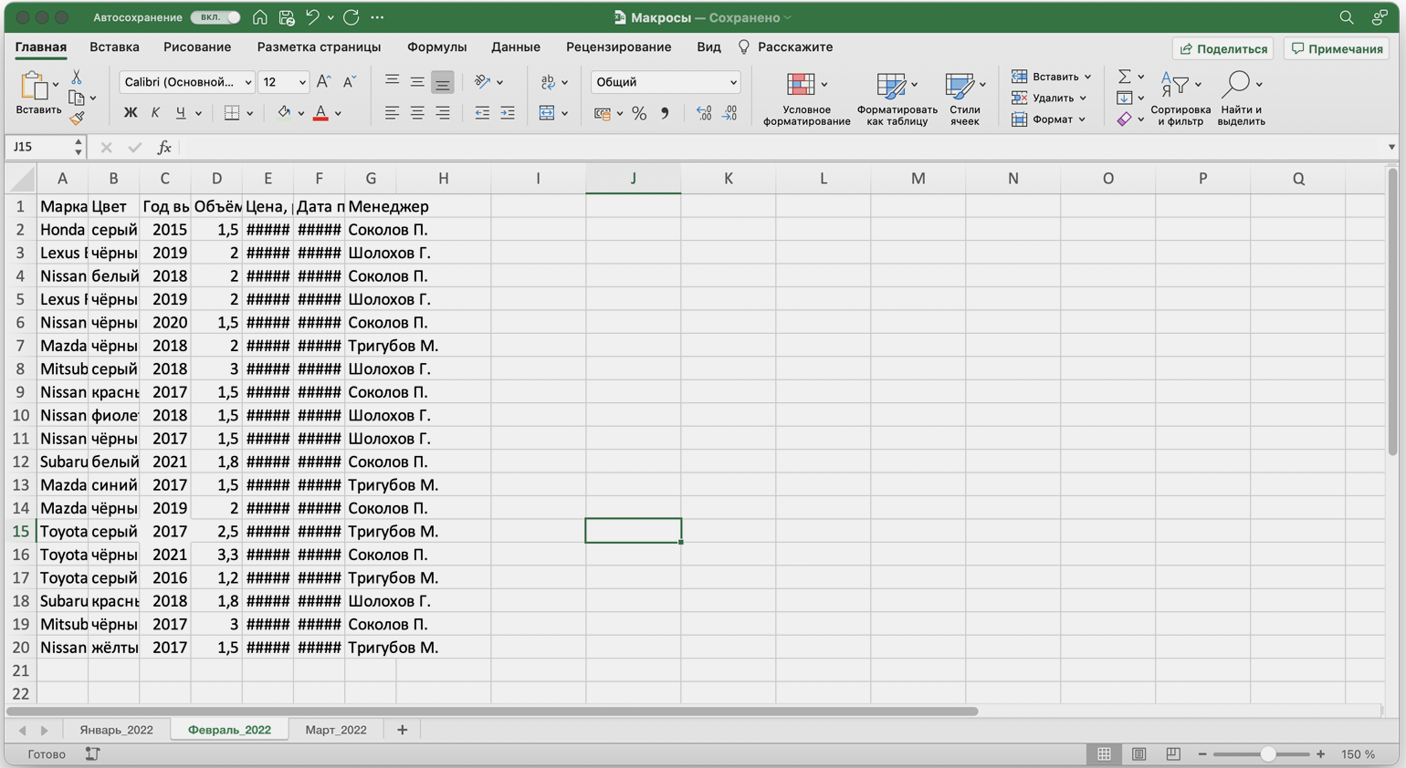
Скриншот: Skillbox Media
Пользоваться таким отчётом неудобно — нужно сделать его наглядным. Запишем макрос при форматировании таблицы с продажами за январь и затем применим его к двум другим таблицам.
Готовимся к записи макроса
Кнопки для работы с макросами в Excel находятся во вкладке «Разработчик». Эта вкладка по умолчанию скрыта, поэтому для начала разблокируем её.
В операционной системе Windows это делается так: переходим во вкладку «Файл» и выбираем пункты «Параметры» → «Настройка ленты». В открывшемся окне в разделе «Основные вкладки» находим пункт «Разработчик», отмечаем его галочкой и нажимаем кнопку «ОК» → в основном меню Excel появляется новая вкладка «Разработчик».
В операционной системе macOS это нужно делать по-другому. В самом верхнем меню нажимаем на вкладку «Excel» и выбираем пункт «Параметры…».
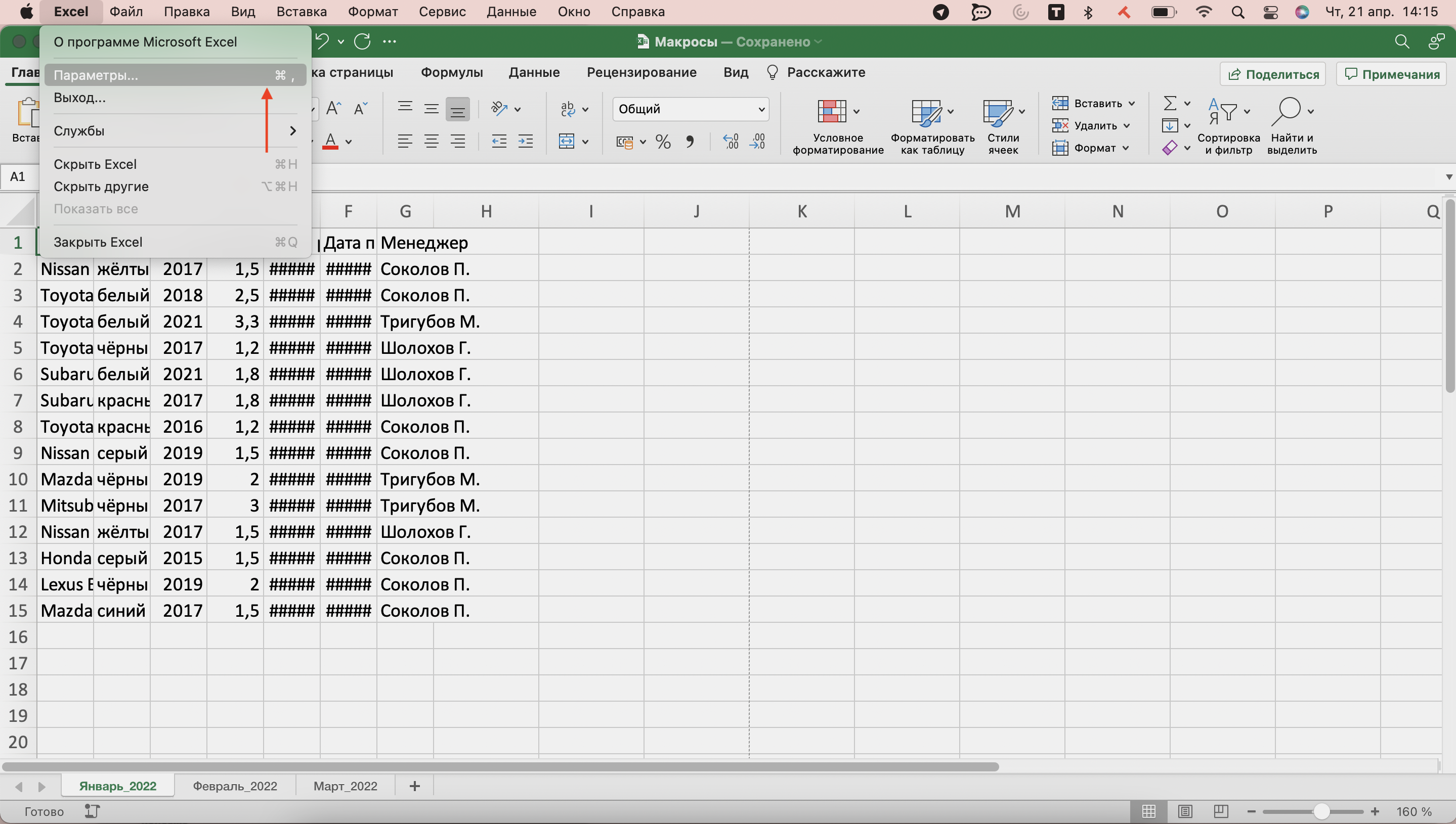
Скриншот: Skillbox Media
В появившемся окне нажимаем кнопку «Лента и панель».
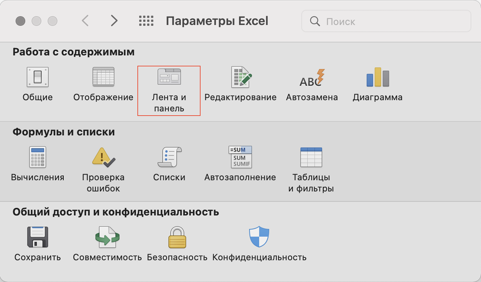
Скриншот: Skillbox Media
Затем в правой панели «Настроить ленту» ищем пункт «Разработчик» и отмечаем его галочкой. Нажимаем «Сохранить».
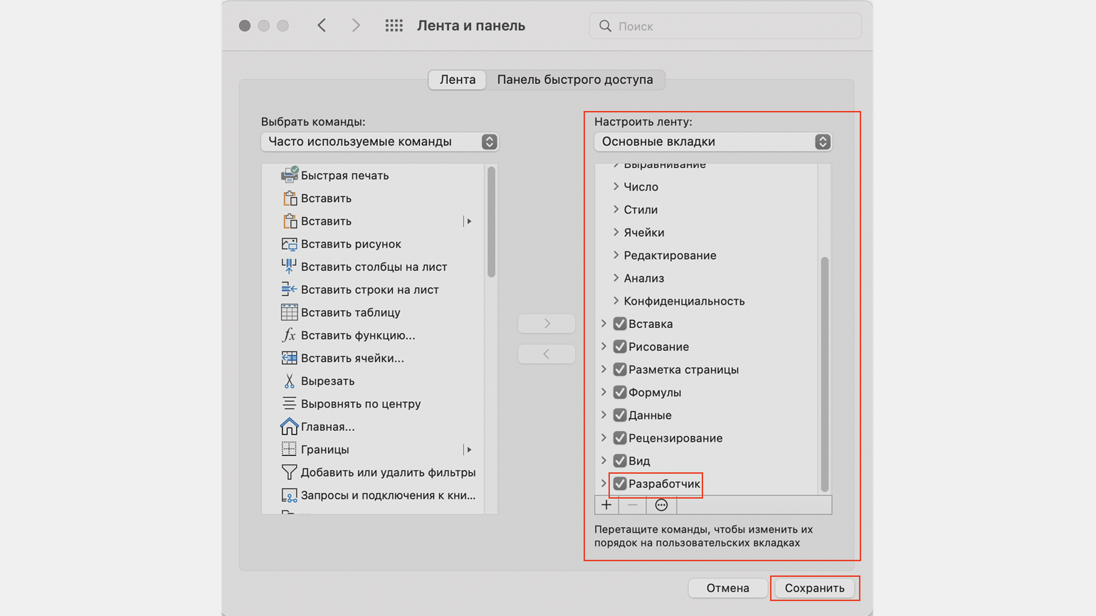
Скриншот: Skillbox Media
Готово — вкладка «Разработчик» появилась на основной панели Excel.
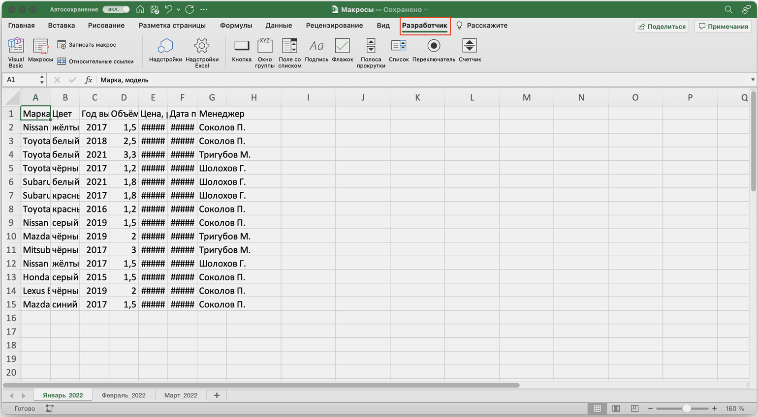
Скриншот: Skillbox Media
Чтобы Excel смог сохранить и в дальнейшем использовать макрос, нужно пересохранить документ в формате, который поддерживает макросы. Это делается через команду «Сохранить как» на главной панели. В появившемся меню нужно выбрать формат «Книга Excel с поддержкой макросов».
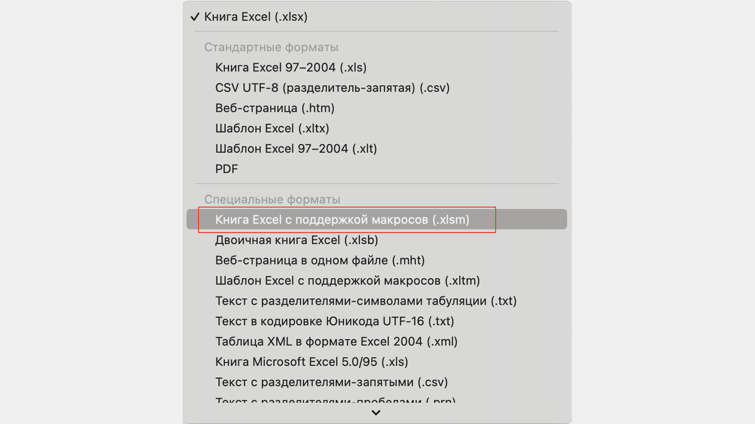
Скриншот: Skillbox Media
Перед началом записи макроса важно знать об особенностях его работы:
- Макрос записывает все действия пользователя.
После старта записи макрос начнёт регистрировать все клики мышки и все нажатия клавиш. Поэтому перед записью последовательности лучше хорошо отработать её, чтобы не добавлять лишних действий и не удлинять код. Если требуется записать длинную последовательность задач — лучше разбить её на несколько коротких и записать несколько макросов.
- Работу макроса нельзя отменить.
Все действия, которые выполняет запущенный макрос, остаются в файле навсегда. Поэтому перед тем, как запускать макрос в первый раз, лучше создать копию всего файла. Если что-то пойдёт не так, можно будет просто закрыть его и переписать макрос в созданной копии.
- Макрос выполняет свой алгоритм только для записанного диапазона таблиц.
Если при записи макроса пользователь выбирал диапазон таблицы, то и при запуске макроса в другом месте он выполнит свой алгоритм только в рамках этого диапазона. Если добавить новую строку, макрос к ней применяться не будет. Поэтому при записи макроса можно сразу выбирать большее количество строк — как это сделать, показываем ниже.
Для начала записи макроса перейдём на вкладку «Разработчик» и нажмём кнопку «Записать макрос».
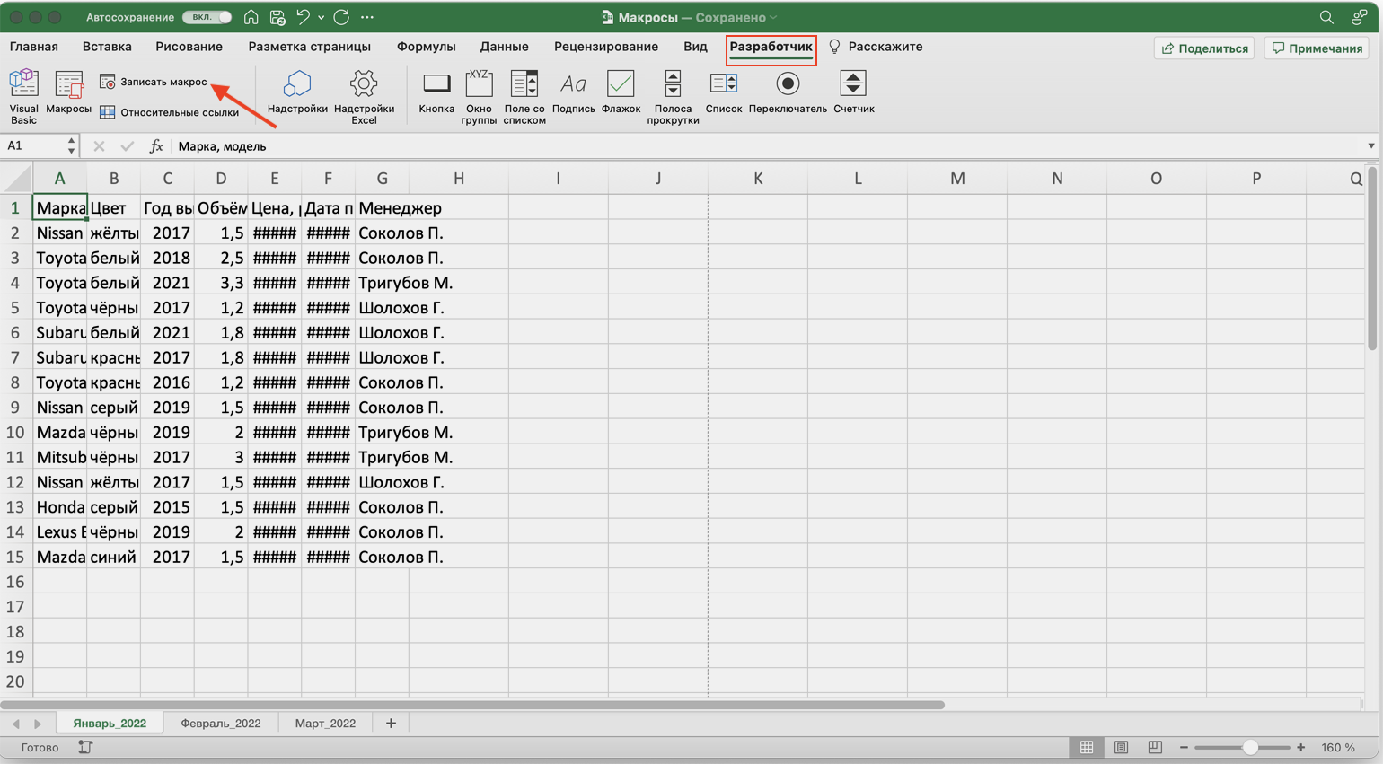
Скриншот: Skillbox Media
Появляется окно для заполнения параметров макроса. Нужно заполнить поля: «Имя макроса», «Сохранить в», «Сочетание клавиш», «Описание».
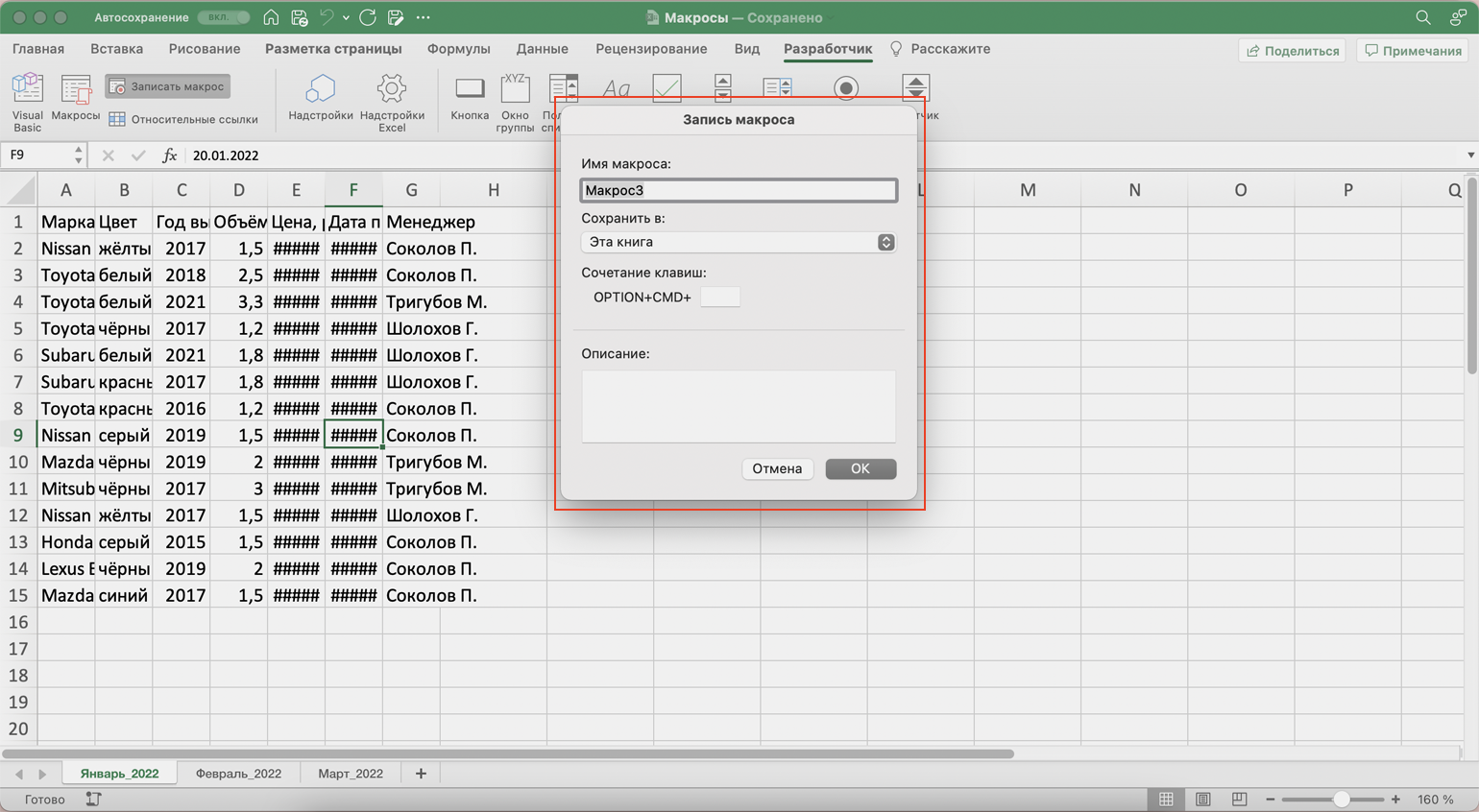
Скриншот: Skillbox Media
«Имя макроса» — здесь нужно придумать и ввести название для макроса. Лучше сделать его логически понятным, чтобы в дальнейшем можно было быстро его найти.
Первым символом в названии обязательно должна быть буква. Другие символы могут быть буквами или цифрами. Важно не использовать пробелы в названии — их можно заменить символом подчёркивания.
«Сохранить в» — здесь нужно выбрать книгу, в которую макрос сохранится после записи.
Если выбрать параметр «Эта книга», макрос будет доступен при работе только в этом файле Excel. Чтобы макрос был доступен всегда, нужно выбрать параметр «Личная книга макросов» — Excel создаст личную книгу макросов и сохранит новый макрос в неё.
«Сочетание клавиш» — здесь к уже выбранным двум клавишам (Ctrl + Shift в системе Windows и Option + Cmd в системе macOS) нужно добавить третью клавишу. Это должна быть строчная или прописная буква, которую ещё не используют в других быстрых командах компьютера или программы Excel.
В дальнейшем при нажатии этих трёх клавиш записанный макрос будет запускаться автоматически.
«Описание» — необязательное поле, но лучше его заполнять. Например, можно ввести туда последовательность действий, которые планируется записать в этом макросе. Так не придётся вспоминать, какие именно команды выполнит этот макрос, если нужно будет запустить его позже. Плюс будет проще ориентироваться среди других макросов.
В нашем случае с форматированием таблицы заполним поля записи макроса следующим образом и нажмём «ОК».
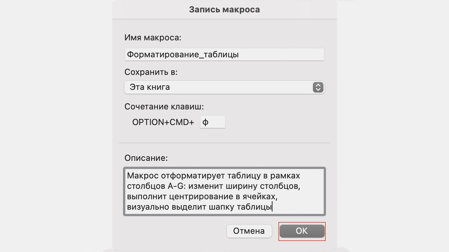
Скриншот: Skillbox Media
После этого начнётся запись макроса — в нижнем левом углу окна Excel появится значок записи.
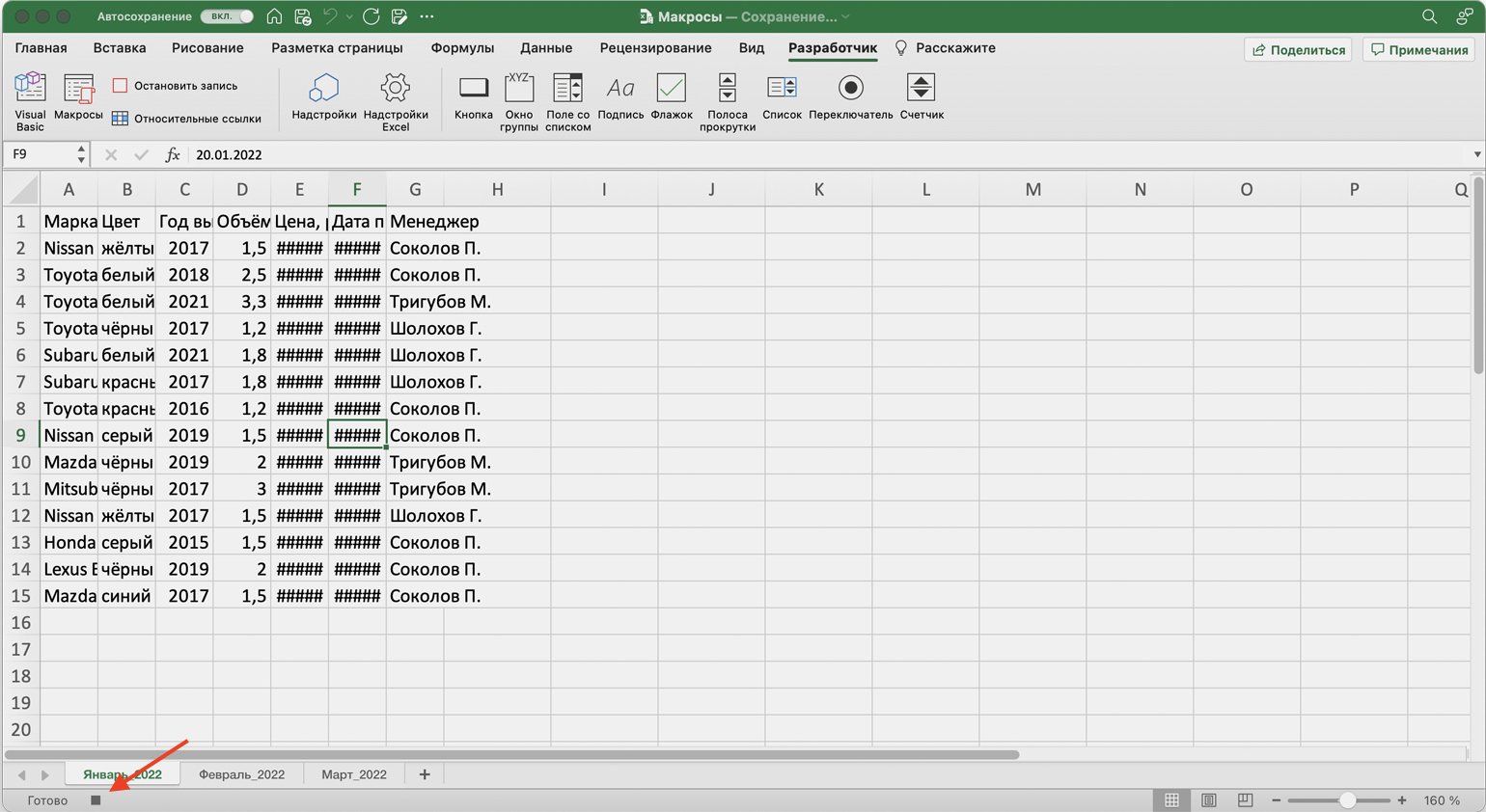
Скриншот: Skillbox Media
Пока идёт запись, форматируем таблицу с продажами за январь: меняем ширину всех столбцов, данные во всех ячейках располагаем по центру, выделяем шапку таблицы цветом и жирным шрифтом, рисуем границы.
Важно: в нашем случае у таблиц продаж за январь, февраль и март одинаковое количество столбцов, но разное количество строк. Чтобы в случае со второй и третьей таблицей макрос сработал корректно, при форматировании выделим диапазон так, чтобы в него попали не только строки самой таблицы, но и строки ниже неё. Для этого нужно выделить столбцы в строке с их буквенным обозначением A–G, как на рисунке ниже.
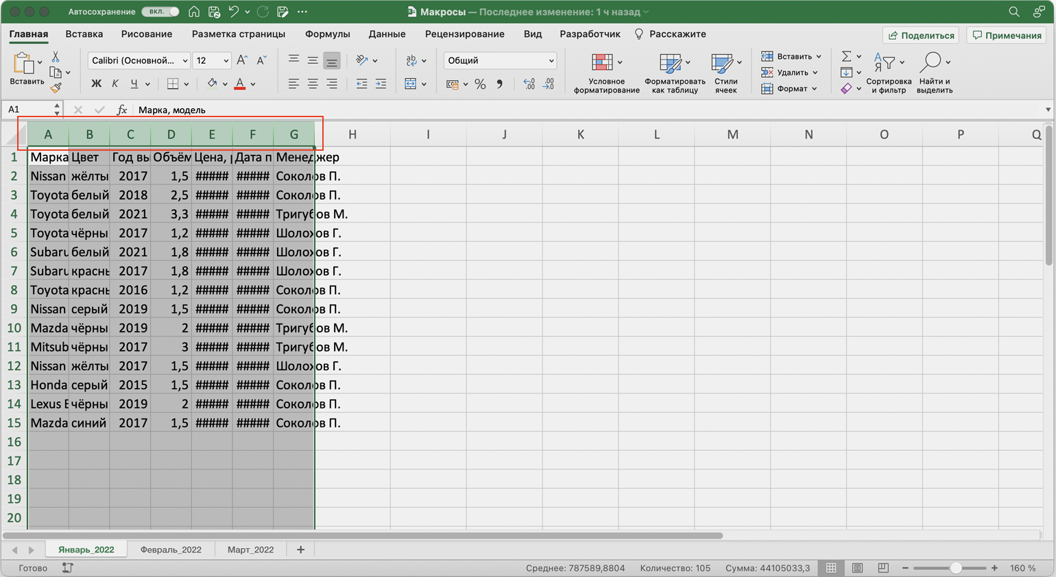
Скриншот: Skillbox Media
Если выбрать диапазон только в рамках первой таблицы, то после запуска макроса в таблице с большим количеством строк она отформатируется только частично.
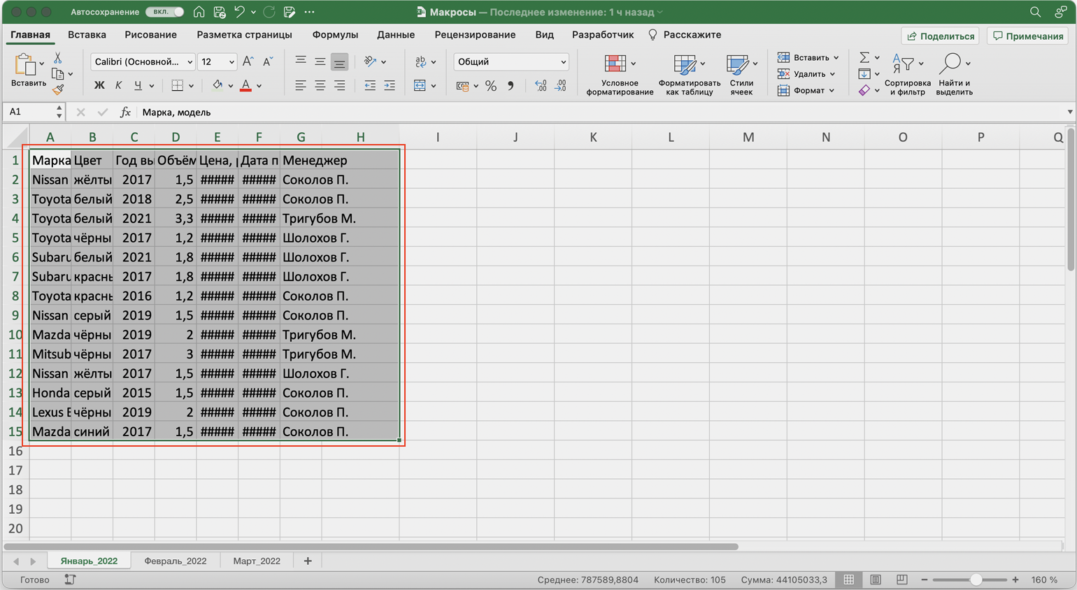
Скриншот: Skillbox Media
После всех манипуляций с оформлением таблица примет такой вид:
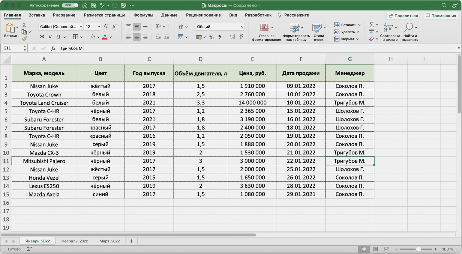
Скриншот: Skillbox Media
Проверяем, все ли действия с таблицей мы выполнили, и останавливаем запись макроса. Сделать это можно двумя способами:
- Нажать на кнопку записи в нижнем левом углу.
- Перейти во вкладку «Разработчик» и нажать кнопку «Остановить запись».
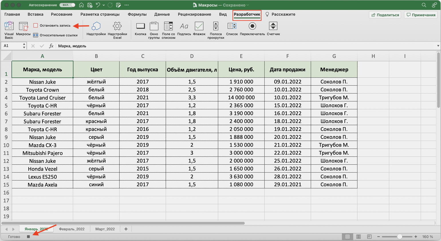
Скриншот: Skillbox Media
Готово — мы создали макрос для форматирования таблиц в границах столбцов A–G. Теперь его можно применить к другим таблицам.
Запускаем макрос
Перейдём в лист со второй таблицей «Февраль_2022». В первоначальном виде она такая же нечитаемая, как и первая таблица до форматирования.
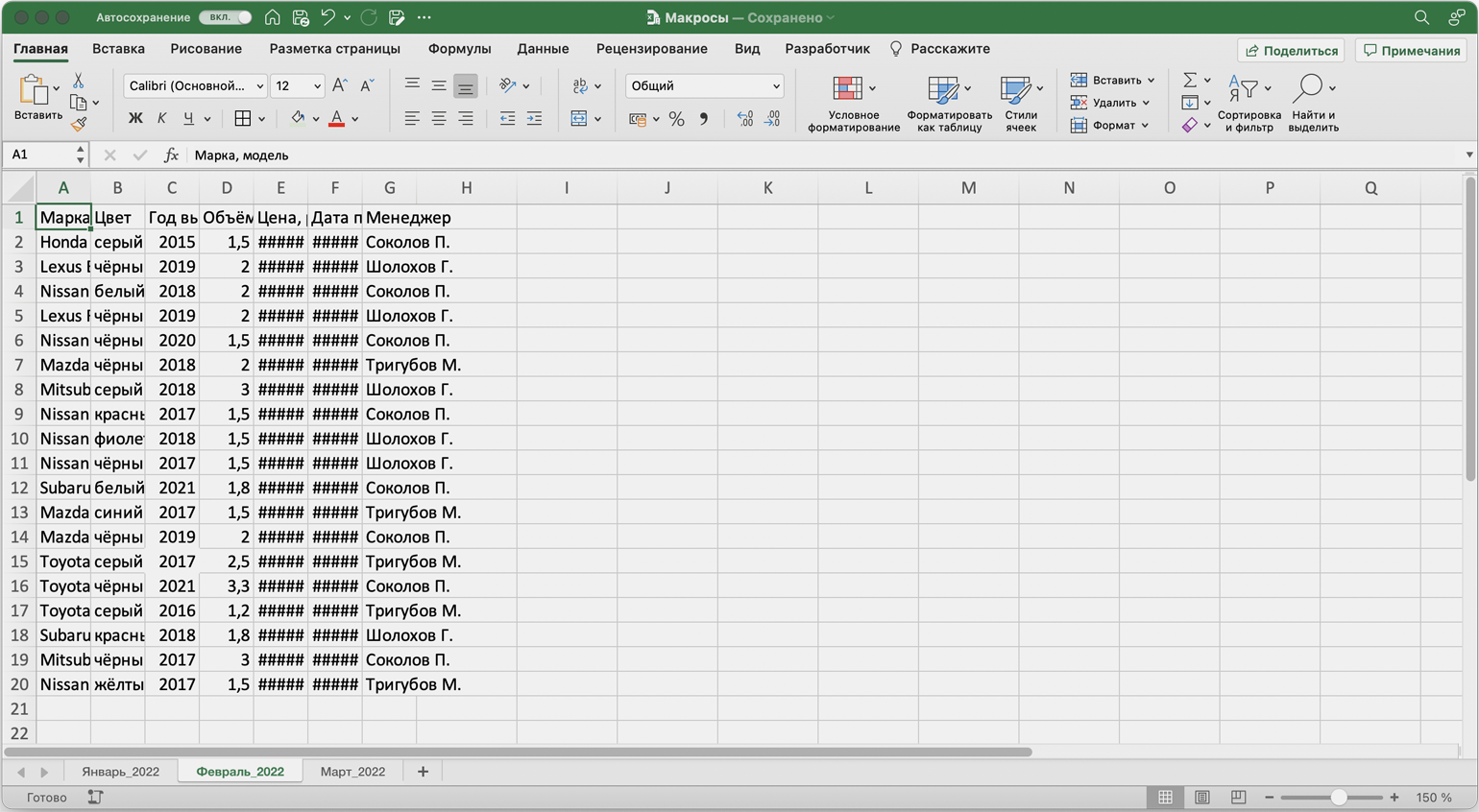
Скриншот: Skillbox Media
Отформатируем её с помощью записанного макроса. Запустить макрос можно двумя способами:
- Нажать комбинацию клавиш, которую выбрали при заполнении параметров макроса — в нашем случае Option + Cmd + Ф.
- Перейти во вкладку «Разработчик» и нажать кнопку «Макросы».
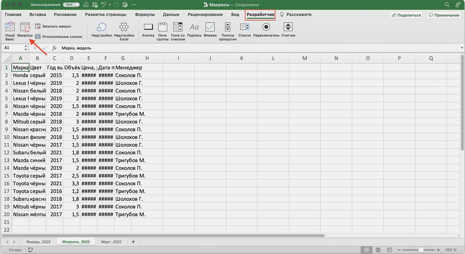
Скриншот: Skillbox Media
Появляется окно — там выбираем макрос, который нужно запустить. В нашем случае он один — «Форматирование_таблицы». Под ним отображается описание того, какие действия он включает. Нажимаем «Выполнить».
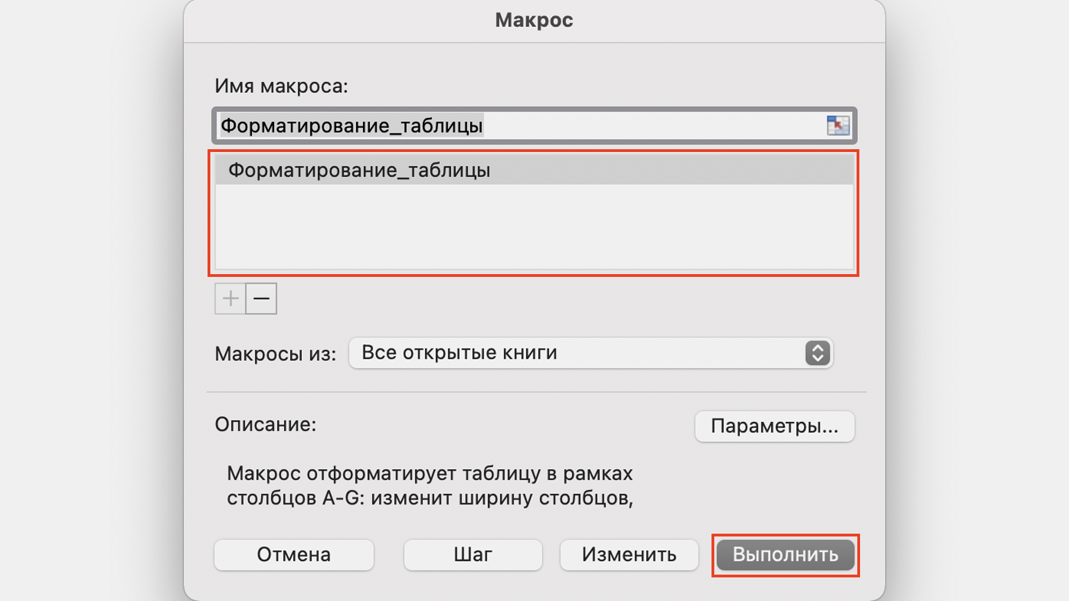
Скриншот: Skillbox Media
Готово — вторая таблица с помощью макроса форматируется так же, как и первая.
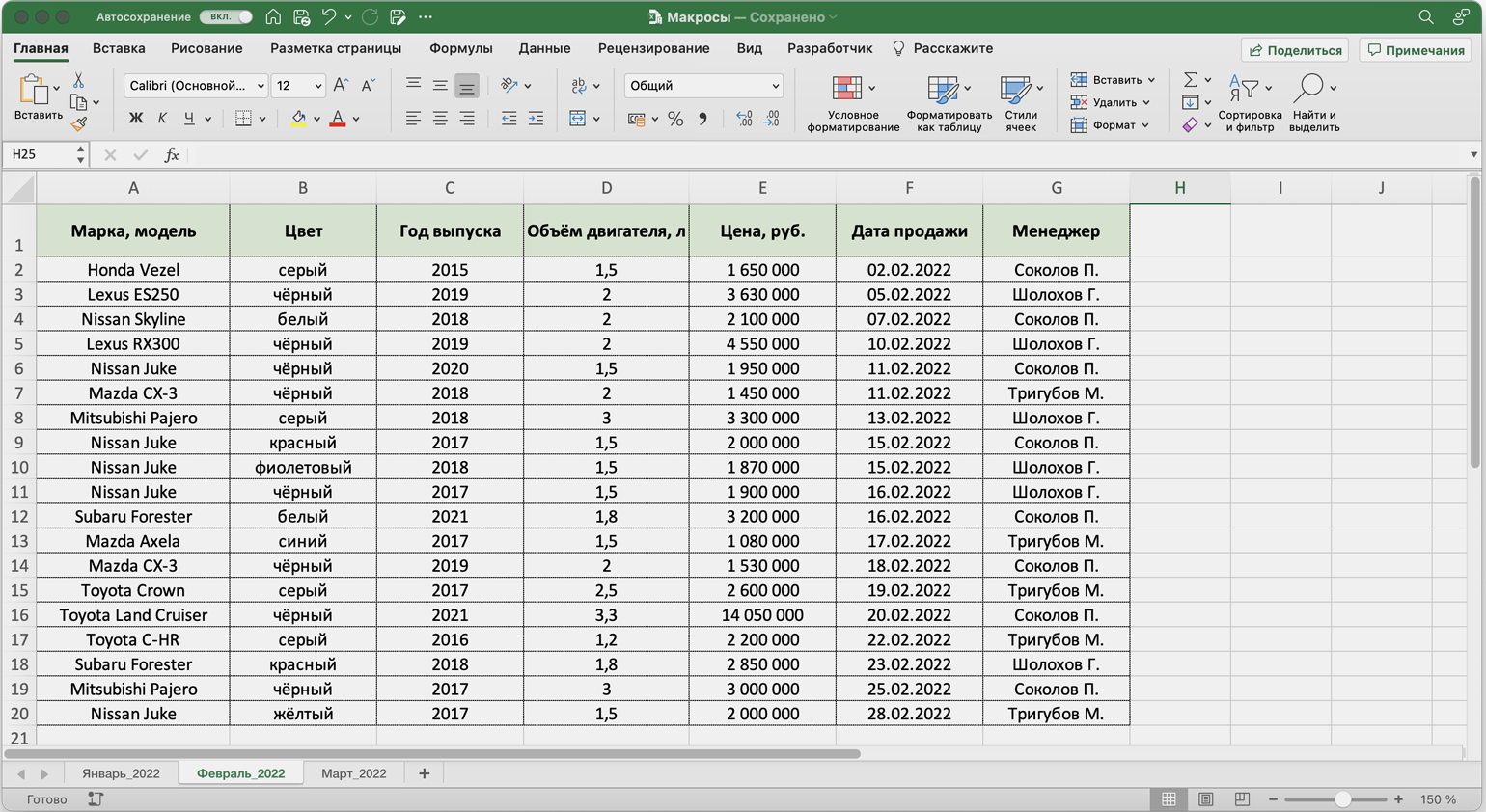
Скриншот: Skillbox Media
То же самое можно сделать и на третьем листе для таблицы продаж за март. Более того, этот же макрос можно будет запустить и в следующем квартале, когда сервис автосалона выгрузит таблицы с новыми данными.

Научитесь: Excel + Google Таблицы с нуля до PRO
Узнать больше