
Excel for Microsoft 365 Excel for Microsoft 365 for Mac Excel for the web Excel 2021 Excel 2021 for Mac Excel 2019 Excel 2019 for Mac Excel 2016 Excel 2016 for Mac Excel 2013 Excel for iPad Excel for iPhone Excel for Android tablets Excel 2010 Excel 2007 Excel for Mac 2011 Excel for Android phones Excel Mobile More…Less
Unlike Microsoft Word, Microsoft Excel doesn’t have a Change Case button for changing capitalization. However, you can use the UPPER, LOWER, or PROPER functions to automatically change the case of existing text to uppercase, lowercase, or proper case. Functions are just built-in formulas that are designed to accomplish specific tasks—in this case, converting text case.
How to Change Case
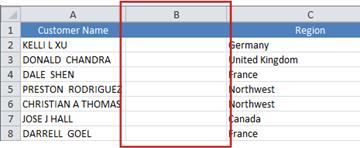
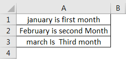
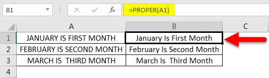
In the example below, the PROPER function is used to convert the uppercase names in column A to proper case, which capitalizes only the first letter in each name.
-
First, insert a temporary column next to the column that contains the text you want to convert. In this case, we’ve added a new column (B) to the right of the Customer Name column.

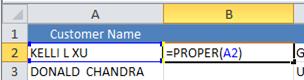
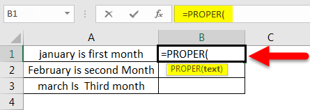
In cell B2, type =PROPER(A2), then press Enter.
This formula converts the name in cell A2 from uppercase to proper case. To convert the text to lowercase, type =LOWER(A2) instead. Use =UPPER(A2) in cases where you need to convert text to uppercase, replacing A2 with the appropriate cell reference.
-
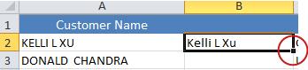
Now, fill down the formula in the new column. The quickest way to do this is by selecting cell B2, and then double-clicking the small black square that appears in the lower-right corner of the cell.
Tip: If your data is in an Excel table, a calculated column is automatically created with values filled down for you when you enter the formula.
-
At this point, the values in the new column (B) should be selected. Press CTRL+C to copy them to the Clipboard.
Right-click cell A2, click Paste, and then click Values. This step enables you to paste just the names and not the underlying formulas, which you don’t need to keep.
-
You can then delete column (B), since it is no longer needed.

Need more help?
You can always ask an expert in the Excel Tech Community or get support in the Answers community.
See Also
Use AutoFill and Flash Fill
Need more help?
You’ve probably come across this situation before.
You have a list of names and it’s all lower case letter. You need to fix them so they are all properly capitalized.
With hundreds of names in your list, it’s going to be a pain to go through and edit first and last names.
Thankfully, there are some easy ways to change the case of any text data in Excel. We can change text to lower case, upper case or proper case where each word is capitalized.
In this post, we’re going to look at using Excel functions, flash fill, power query, DAX and power pivot to change the case of our text data.
Video Tutorial
Using Excel Formulas To Change Text Case
The first option we’re going to look at is regular Excel functions. These are the functions we can use in any worksheet in Excel.
There’s a whole category of Excel functions to deal with text, and these three will help us to change the text case.
LOWER Excel Worksheet Function
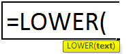
=LOWER(Text)The LOWER function takes one argument which is the bit of Text we want to change into lower case letters. The function will evaluate to text that is all lower case.
UPPER Excel Worksheet Function
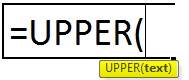
=UPPER(Text)The UPPER function takes one argument which is the bit of Text we want to change into upper case letters. The function will evaluate to text that is all upper case.
PROPER Excel Worksheet Function
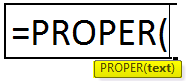
=PROPER(Text)The PROPER function takes one argument which is the bit of Text we want to change into proper case. The function will evaluate to text that is all proper case where each word starts with a capital letter and is followed by lower case letters.
Copy And Paste Formulas As Values
After using the Excel formulas to change the case of our text, we may want to convert these to values.
This can be done by copying the range of formulas and pasting them as values with the paste special command.
Press Ctrl + C to copy the range of cells ➜ press Ctrl + Alt + V to paste special ➜ choose Values from the paste options.
Using Flash Fill To Change Text Case
Flash fill is a tool in Excel that helps with simple data transformations. We only need to provide a couple examples of the results we want, and flash fill will fill in the rest.
Flash fill can only be used directly to the right of the data we’re trying to transform. We need to type out a couple of examples of the results we want. When Excel has enough examples to figure out the pattern, it will show the suggested data in a light grey font. We can accept this suggested filled data by pressing Enter.
We can also access flash fill from the ribbon. Enter the example data ➜ highlight both the examples and cells that need to be filled ➜ go to the Data tab ➜ press the Flash Fill command found in the Data Tools section.
We can also use the keyboard shortcut Ctrl + E for flash fill.
Flash fill will work for many types of simple data transformations including changing text between lower case, upper case and proper case.
Using Power Query To Change Text Case
Power query is all about data transformation, so it’s sure there is a way to change the case of text in this tool.
With power query we can transform the case into lower, upper and proper case.
Select the data we want to transform ➜ go to the Data tab ➜ select From Table/Range. This will open up the power query editor where we can apply our text case transformations.
Text.Lower Power Query Function
Select the column containing the data we want to transform ➜ go to the Add Column tab ➜ select Format ➜ select lowercase from the menu.
= Table.AddColumn(#"Changed Type", "lowercase", each Text.Lower([Name]), type text)This will create a new column with all text converted to lower case letters using the Text.Lower power query function.
Text.Upper Power Query Function
Select the column containing the data we want to transform ➜ go to the Add Column tab ➜ select Format ➜ select UPPERCASE from the menu.
= Table.AddColumn(#"Changed Type", "UPPERCASE", each Text.Upper([Name]), type text)This will create a new column with all text converted to upper case letters using the Text.Upper power query function.
Text.Proper Power Query Function
Select the column containing the data we want to transform ➜ go to the Add Column tab ➜ select Format ➜ select Capitalize Each Word from the menu.
= Table.AddColumn(#"Changed Type", "Capitalize Each Word", each Text.Proper([Name]), type text)This will create a new column with all text converted to proper case lettering, where each word is capitalized, using the Text.Proper power query function.
Using DAX Formulas To Change Text Case
When we think of pivot tables, we generally think of summarizing numeric data. But pivot tables can also summarize text data when we use the data model and DAX formulas. There are even DAX formula to change text case before we summarize it!
First, we need to create a pivot table with our text data. Select the data to be converted ➜ go to the Insert tab ➜ select PivotTable from the tables section.
In the Create PivotTable dialog box menu, check the option to Add this data to the Data Model. This will allow us to use the necessary DAX formula to transform our text case.
Creating a DAX formula in our pivot table can be done by adding a measure. Right click on the table in the PivotTable Fields window and select Add Measure from the menu.
This will open up the Measure dialog box, where we can create our DAX formulas.
LOWER DAX Function
=CONCATENATEX( ChangeCase, LOWER( ChangeCase[Mixed Case] ), ", ")We can enter the above formula into the Measure editor. Just like the Excel worksheet functions, there is a DAX function to convert text to lower case.
However, in order for the expression to be a valid measure, it will need to be wrapped in a text aggregating function like CONCATENATEX. This is because measures need to evaluate to a single value and the LOWER DAX function does not do this on it’s own. The CONCATENATEX function will aggregate the results of the LOWER function into a single value.
We can then add the original column of text into the Rows and the new Lower Case measure into the Values area of the pivot table to produce our transformed text values.
Notice the grand total of the pivot table contains all the names in lower case text separated by a comma and space character. We can hide this part by going to the Table Tools Design tab ➜ Grand Totals ➜ selecting Off for Rows and Columns.
UPPER DAX Function
=CONCATENATEX( ChangeCase, UPPER( ChangeCase[Mixed Case] ), ", ")Similarily, we can enter the above formula into the Measure editor to create our upper case DAX formula. Just like the Excel worksheet functions, there is a DAX function to convert text to upper case.
Creating the pivot table to display the upper case text is the same process as with the lower case measure.
Missing PROPER DAX Function
We might try and create a similar DAX formula to create proper case text. But it turns out there is no function in DAX equivalent to the PROPER worksheet function.
Using Power Pivot Row Level Formulas To Change Text Case
This method will also use pivot tables and the Data Model, but instead of DAX formulas we can create row level calculations using the Power Pivot add-in.
Power pivot formulas can be used to add new calculated columns in our data. Calculations in these columns happen for each row of data similar to our regular Excel worksheet functions.
Not every version of Excel has power pivot available and you will need to enable the add-in before you can use it. To enable the power pivot add-in, go to the File tab ➜ Options ➜ go to the Add-ins tab ➜ Manage COM Add-ins ➜ press Go ➜ check the box for Microsoft Power Pivot for Excel.
We will need to load our data into the data model. Select the data ➜ go to the Power Pivot tab ➜ press the Add to Data Model command.
This is the same data model as creating a pivot table and using the Add this data to the Data Model checkbox option. So if our data is already in the data model we can use the Manage data model option to create our power pivot calculations.
LOWER Power Pivot Function
=LOWER(ChangeCase[Mixed Case])Adding a new calculated column into the data model is easy. Select an empty cell in the column labelled Add Column then type out the above formula into the formula bar. You can even create references in the formula to other columns by clicking on them with the mouse cursor.
Press Enter to accept the new formula.
The formula will appear in each cell of the new column regardless of which cell was selected. This is because each row must use the same calculation within a calculated column.
We can also rename our new column by double clicking on the column heading. Then we can close the power pivot window to use our new calculated column.
When we create a new pivot table with the data model, we will see the calculated column as a new available field in our table and we can add it into the Rows area of the pivot table. This will list out all the names in our data and they will all be lower case text.
UPPER Power Pivot Function
=UPPER(ChangeCase[Mixed Case])We can do the same thing to create a calculated column that converts the text to upper case by adding a new calculated column with the above formula.
Again, we can then use this as a new field in any pivot table created from the data model.
Missing PROPER Power Pivot Function
Unfortunately, there is no power pivot function to convert text to proper case. So just like DAX, we won’t be able to do this in a similar fashion to the lower case and upper case power pivot methods.
Conclusions
There are many ways to change the case of any text data between lower, upper and proper case.
- Excel Formulas are quick, easy and will dynamically update if the inputs ever change.
- Flash fill is great for one-off transformations where you need to quickly fix some text and don’t need to update or change the data after.
- Power query is perfect for fixing data that will be imported regularly into Excel from an outside source.
- DAX and power pivot are can be used for fixing text to display within a pivot table.
Each option has different strengths and weaknesses so it’s best to become familiar will all methods so you can choose the one that will best suit your needs.
About the Author
John is a Microsoft MVP and qualified actuary with over 15 years of experience. He has worked in a variety of industries, including insurance, ad tech, and most recently Power Platform consulting. He is a keen problem solver and has a passion for using technology to make businesses more efficient.
How to Change Case in Excel: Upper, Lower, and More (2023)
Sometimes, you need to change the letter case of a text for proper capitalization of names, places, and things. In Microsoft Word, it’s easy to do that using the Change Case button.
However, there is no Change Case button in Microsoft Excel 🙁 Then how do you change the letter case of texts in Excel? How much more if you need to change the letter case of texts of large data sets? 😱
Good news! Changing the letter case of text is possible in Excel, and you don’t have to manually do it at all!
Excel offers you the UPPER, LOWER, and PROPER functions to automatically change text values to upper case, lower case, or proper case 😊
Let’s do it!
Before you scroll down, make sure to download this free practice workbook we’ve prepared for you to work on.
How to change case to uppercase
To change the case of text into uppercase means to capitalize all lowercase letters in a text string. Simply put, to change them to ALL CAPS.
You can do this in Excel by using the UPPER function. It has the following syntax:
=UPPER(text)
The only argument in this function is the text. It refers to the text that you want to be converted to uppercase. This can be a reference or text string.
It’s time to open your practice workbook and put this function into action 💪
You will see a column named Original Data which contains names, places, and sentences that are written in different text case formats.
You may have encountered this in real life where you have to work with data that do not appear in a format that you want.
Let’s convert text data in the original data column into uppercase using the UPPER function.
- Double-click on cell B2 to put the cell in Edit mode.

- Type the UPPER function:
=UPPER(

- The first and only argument in the UPPER function is the text. You can type in the text string or simply click the cell reference of the text you want to convert to uppercase 😊
In our case, click cell A2. Close the formula with a right parenthesis.
The formula should now look like this:
=UPPER(A2)

- Press Enter.

You have successfully changed the text case to all caps 👍
- Fill in the rest of the rows by dragging down the fill handle or double-clicking it.

All caps in no time!
You don’t have to worry about converting text in large data sets into uppercase. The UPPER function is all you need!
But what if you need to capitalize only the first letter of the text, not all the text characters of the whole text string? 🤔No worries, Excel can help you do that too using the PROPER function!
Capitalize the first letter using the PROPER function
As the name of the function suggests, the PROPER function converts text into proper form or case. It only capitalizes the first letter of each substring of text.
The text could be a single word. It could also be multiple words such as first and last names, cities and states, abbreviations, suffixes, and honorifics/titles.
The PROPER function follows the same syntax and arguments as the UPPER and LOWER functions:
=PROPER(text)
In a new column of our practice workbook, let’s convert the text string to the proper case 😊
- Double-click cell C2.

- Type the PROPER function:
=PROPER(

- Click cell A2 as your text. Then close the formula with a right parenthesis.
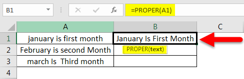
=PROPER(A2)

- Press Enter. Fill in the rest of the rows using the fill handle.

Only the first letter of each of the substrings of the whole text string is capitalized.
As mentioned above, this works best in converting first and last names, cities and states, abbreviations, and more.
You can convert the text in Microsoft Excel into the proper case in no time! 😀
Pro Tip!
Excel automatically suggests formulas as you type.
For example, you can just type “=pro” and the suggestion for “=PROPER” will appear.
Press the Tab key to input the suggested formula.
How to change case to lowercase
If you have a list that comes in all caps, you can convert them all to lowercase using the LOWER function.
This is the syntax of the LOWER function:
=LOWER(text)
Remember Column B in our practice workbook where we placed all converted uppercase text? Let’s convert that to lowercase letters.
Let’s create a new column where we will place the text converted to lowercase 👇

- Start by double-clicking cell D2.

- Type the formula:
=LOWER(B2)

- Press Enter. Fill in the other rows by double-clicking the fill handle or dragging it down.

Now all text is now in lowercase letters 👍
This is how your practice workbook should look overall ✨
Comparing the data in the original column, you can convert any text data into upper case, proper case, or lower case.

For UPPER and LOWER functions, it would just change all the text characters to upper case or lower case.
For the PROPER function, there are a couple of limitations you need to be aware of ✍
As you know, it only capitalizes the first character in a text string. The limitation is that it does not know the difference between an actual word and an abbreviation – like an acronym for instance.
For example, if we apply the PROPER function to something like “FIFA”, it will return “Fifa”.
Another example would be using the suffix “md” for a medical doctor. If we apply the PROPER function to it, it will return “Md”.
This is not the desired outcome and should be kept in mind 💭
That’s it – Now what?
Nice work! Now you know how to convert text into upper, proper, and lower letter cases. You won’t have to worry about changing letter cases of large sets of data, and no more manual typing 🥳
Convert text like a pro, get work done faster, and impress your boss with this advanced skill in Microsoft Excel.
There are still so many functions in Excel that will help you save a lot of work. Learn functions you actually NEED like the IF, the SUMIF, and the most popular Excel function: the VLOOKUP function 🚀
You might be thinking 🤔 if there is an easy and quick way to learn these.
Of course! Join my FREE Excel Intermediate Training where I send you free lessons about the IF, SUMIF, and VLOOKUP function. Plus, you’ll learn how to effectively clean your data in Excel too.
Click here to join 😀
Other resources
Do you want to extract text substrings in Excel instead? Learn exactly with LEFT, RIGHT, and MID Functions in Excel. Read more here.
You can also learn how to convert numbers or dates to text to increase their readability or to bring them to a certain format. You can do that using the TEXT function in Excel! Read about Excel’s TEXT function here.
I hope this was a helpful read 👋
Frequently asked questions
You can use the UPPER function to convert small letters to capital letters.
- In a cell, type “=UPPER(“
- Click the cell reference of the text you want to convert to capital letters, then close the formula with a right parenthesis.
- Press Enter.
Kasper Langmann2023-02-23T14:55:02+00:00
Page load link
Changing Case of Text in Excel
Excel provided a set of options to deal with text. But, there is a problem with Excel. It does not have the option to change the case of the text in Excel worksheets. Instead, it provides three major functions to convert the text to lower, upper, and proper cases. It helps to minimize the problems in changing the cases. This article will teach how to change text cases in Excel.
Table of contents
- Changing Case of Text in Excel
- Functions used to Change Case in Excel
- #1 – Lowercase in Excel
- #2 – Uppercase in Excel
- #3 – Proper Case in Excel
- How to Change Case in Excel? (with Examples)
- Example#1: Change Text to Lowercase using the LOWER function
- Example#2: Converting Text to Uppercase Using UPPER function
- Example#3: Converting Text to Title case Using the PROPER function
- Example#4: Changing the Text Using the Flash Fill Method
- Things to Remember
- Recommended Articles
- Functions used to Change Case in Excel
Functions used to Change Case in Excel
The following are the functions used to change text case in Excel:
#1 – Lowercase in Excel
Use the LOWER function to convert all the text presented in a cell to lowercase. Use the following formula:
#2 – Uppercase in Excel
Use the UPPER function to convert all the text presented in a cell to uppercase. Use the following formula:
#3 – Proper Case in Excel
Use the PROPER function to convert all the text presented in a cell to the title case. Use the following formula:
WE should select only one cell to apply the change case functions. When a formula is entered, the hover is displayed by mentioning the purpose of the function. After entering a formula, we should press the “ENTER” key on the keyboard to have the desired result.
How to Change Case in Excel? (with Examples)
The change case functions are used in two ways in Excel:
- First method: Directly enter the function name in a cell.
- Second method: Insert the functions from the “Formula” tab.
The following are some examples to understand how to change the case.
Example#1: Change Text to Lowercase using the LOWER function
The following example is considered to explain the use of the LOWER function. Several steps are required to display the text in the required format.
- Step 1: We must select the cell where you want to converts the text case in Excel into lowercase There are six methods to change lowercase in excel — Using the lower function to change case in excel, Using the VBA command button, VBA shortcut key, Using Flash Fill, Enter text in lower case only, Using Microsoft word.
read more.
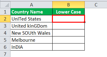
The above figure shows the sample data converted into a lower case. We should enter the formula of the lower function into the highlighted cell.
- Step 2: First, we must go to the top of the ribbon and click on the “Formula” tab to select the function, as shown in the image. The LOWER (text) description is displayed by hovering on the function.
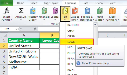
- Step 3: Once we click on a LOWER function, the function argument window will open.
- Step 4: The cell address should be entered into the function arguments box, and the results should be displayed in the figure.
Now, press the “Enter” key to see the change in the text case.
- Step 5: Now, we will drag the formula to apply to the remaining cells to convert the data presented in the next rows.

Example#2: Converting Text to Uppercase Using UPPER function
The following example is considered to explain the use of the UPPER function. Several steps are required to display the text in the capitalized format.
- Step 1: We must select the cell we want to convert into the upper case.

The above figure shows the sample data to convert into the upper case. But, first, we should enter the basic Excel formulasThe term «basic excel formula» refers to the general functions used in Microsoft Excel to do simple calculations such as addition, average, and comparison. SUM, COUNT, COUNTA, COUNTBLANK, AVERAGE, MIN Excel, MAX Excel, LEN Excel, TRIM Excel, IF Excel are the top ten excel formulas and functions.read more of the upper function into the highlighted cell.
- Step 2: We must go to the top of the ribbon and click on the “Formula” tab to select the function, as shown in the image. The UPPER (text) description is displayed by hovering on the function.
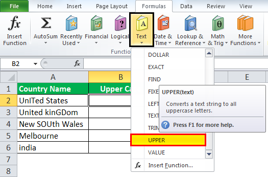
- Step 3: Once we click on an UPPER function, the “Function Arguments” window will open. The UPPER function is found among the several functions available.
- Step 4: The cell address should be entered into the “Function Arguments” box, and the result should be displayed in the figure.
Now, press the “Enter” key to see the change in the text case.
- Step 5: We will drag the formula to apply to the remaining cells to convert the data presented in the next rows.
Example#3: Converting Text to Title case Using the PROPER function
The following example is considered to explain the use of the PROPER in the ExcelThe Proper Excel function converts the given input to proper case, which means that the first character in a word is in uppercase and the rest of the characters are in lower case. To use this function type =PROPER( and provide string as input).read more function. Several steps are required to display the text in the title case.
- Step 1: We must select the cell we want to convert into a title case.
The above figure shows the sample data to convert into a title case. We should enter the formula of the title function into the highlighted cell.
- Step 2: We must go to the top of the ribbon and click on the “Formula” tab to select the function, as shown in the image. The description for the PROPER (text) is displayed by hovering on the function.
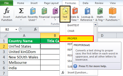
- Step 3: Once we click on a PROPER function, the “Function Arguments” window will open. The PROPER function is found among the several functions available.
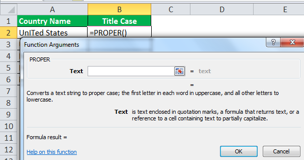
- Step 4: We must insert the cell address into the “Function Arguments” box, and the result is displayed in the figure.

Now, press the “Enter” key to see the change in the text case.
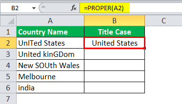
- Step 5: Next, we will drag the formula to apply to the remaining cells to convert the data presented in the next rows.
Example#4: Changing the Text Using the Flash Fill Method
- Step 1: We must type the data in lower case to convert it into upper case.

- Step 2: Now, type the same data in a highlighted cell in the UPPER case and press the “ENTER” key to move the cursor to the below cell.
- Step 3:
- Go to the “Data” tab and click on the ‘Flash Fill’ option in Excel under the “Data Tools” group. The remaining data is automatically typed by converting it into the UPPER case, as shown in the below figure.
Things to Remember
- The change case functions such as LOWER, UPPER, and PROPER do not work on the numerical data, special characters, and punctuation.
- While using a PROPER function, the “S” letter after the apostrophe is converted into the uppercase. So here, we should convert letters manually into lowercase.
- The change case functions accept only one input at a time. Therefore, it is hard to change the case of text presented in all cells.
- There is no option to select only the particular text to change the case.
Recommended Articles
This article is a guide to Change Case in Excel. We discuss how to change text case in Excel using LOWER, UPPER, PROPER, and FLASH FILL functions with examples. You may also look at these useful functions in Excel: –
- Insert Delta Symbol in ExcelIn Excel, Delta symbol is used over time to show change. This is used to create dashboards with eye-catching colors. There are two types of delta symbols like the Filled delta symbol and the empty delta symbol. Auto-correction is the best option if the delta symbol is using continuously. The user can insert the Delta symbol (Δ) in excel using the Insert option, ALT + 30 shortcut key, changing the font name, CHAR formula, excel AutoCorrect feature or custom number formatting with Delta symbol.read more
- $ Symbol in Excel
- Chi-Square Test in ExcelIn Excel, the Chi-Square test is the most commonly used non-parametric test for comparing two or more variables for randomly selected data. It is a test that is used to determine the relationship between two or more variables.read more
- Excel The toolbar, also known as the quick access toolbar, is located on the left top-most side of the excel window and has only a few options by default, such as save, redo, and undo. Users can, however, customize it to their liking and add any option or button to make it easier to access the commands.read moreToolBarThe toolbar, also known as the quick access toolbar, is located on the left top-most side of the excel window and has only a few options by default, such as save, redo, and undo. Users can, however, customize it to their liking and add any option or button to make it easier to access the commands.read more
![]()
Download Article
![]()
Download Article
When you’re working with improperly-capitalized data in Microsoft Excel, there’s no need to make manual corrections! Excel comes with two text-specific functions that can really be helpful when your data is in the wrong case. To make all characters appear in uppercase letters, you can use a simple function called UPPERCASE to convert one or more cells at a time. If you need your text to be in proper capitalization (first letter of each name or word is capitalized while the rest is lowercase), you can use the PROPER function the same way you’d use UPPERCASE. This wikiHow teaches you how to use the UPPERCASE and PROPER functions to capitalize your Excel data.
Steps
-
1
Type a series of text in a column. For example, you could enter a list of names, artists, food items—anything. The text you enter can be in any case, as the UPPERCASE or PROPER function will correct it later.[1]
-
2
Insert a column to the right of your data. If there’s already a blank column next to the column that contains your data, you can skip this step. Otherwise, right-click the column letter above your data column and select Insert.
- You can always remove this column later, so don’t worry if it messes up the rest of your spreadsheet right now.
Advertisement
-
3
Click the first cell in your new column. This is the cell to the right of the first cell you want to capitalize.
-
4
Click fx. This is the function button just above your data. The Insert Function window will expand.
-
5
Select the Text category from the menu. This displays Excel functions that pertain to handling text.
-
6
Select UPPER from the list. This function converts all letters to uppercase.
- If you’d rather just capitalize the first character of each part of a name (or the first character of each word, if you’re working with words), select PROPER instead.
- You could also use the LOWER function to convert all characters to lowercase.
-
7
Click OK. Now you’ll see «UPPER()» appear in the cell you clicked earlier. The Function Arguments window will also appear.
-
8
Highlight the cells you want to make uppercase. If you want to make everything in the column uppercase, just click the column letter above your data. A dotted line will surround the selected cells, and you’ll also see the range appear in the Function Arguments window.
- If you’re using PROPER, select all of the cells you want to make proper case—the steps are the same no matter which function you’re using.
-
9
Click OK. Now you’ll see the uppercase version of the first cell in your data appear at the first cell of your new column.
-
10
Double-click the bottom-right corner of the cell that contains your formula. This is the cell at the top of the column you inserted. Once you double-click the dot at the bottom of this cell, the formula will propagate to the remaining cells in the column, displaying the uppercase versions of your original column data.
- If you have trouble double-clicking that bottom-right corner, you can also drag that corner all the way down the column until you’ve reached the end of your data.
-
11
Copy the contents of your new column. For example, if your new column (the one that contains the now-uppercase versions of your original data) is column B, you’ll right-click the B above the column and select Copy.
-
12
Paste the values of the copied column over your original data. You’ll need to use a feature called Paste Values, which is different than traditional pasting. This option will replace your original data with just the uppercase versions of each entry (not the formulas). Here’s how to do it:
- Right-click the first cell in your original data. For example, if you started typing names or words into A1, you’d right-click A1.
- The Paste Values option might be in a different place, depending on your version of Excel. If you see a Paste Special menu, click that, select Values, and then click OK.
- If you see an icon with a clipboard that says «123,» click that to paste the values.
- If you see a Paste menu, select that and click Values.
-
13
Delete the column you inserted. Now that you’ve pasted the uppercase versions of your original data over that data, you can delete the formula column without harm. To do so, right-click the letter above the column and click Delete.


Advertisement

Add New Question
-
Question
Can I change to uppercase for an entire working sheet at one time?

Yes, you can do this by selecting the entire sheet then specifying you want it to be uppercase.
-
Question
How do I do uppercase when putting in a password?
You can’t use caps lock on some operating systems; try using the uppercase button
Ask a Question
200 characters left
Include your email address to get a message when this question is answered.
Submit
Advertisement
Thanks for submitting a tip for review!
About This Article
Article SummaryX
You can use the «UPPER» function in Microsoft Excel to transform lower-case letters to capitals. Start by inserting a blank column to the right of the column that contains your data. Click the first blank cell of the new column. Then, click the formula bar at the top of your worksheet—it’s the typing area that has an «fx» on its left side. Type an equal (=) sign, followed by the word «UPPER» in all capital letters. To tell the «UPPER» function which data to convert, click the first cell in your original data column. Press the Enter or Return key on your keyboard to apply the formula. The first cell of your original data column is now converted to uppercase letters. To apply this change to the entire column, click the cell containing the uppercase letters to select it. Then, drag the small square at the bottom-right corner of the cell down to the final row.
Did this summary help you?
Thanks to all authors for creating a page that has been read 1,463,548 times.
Is this article up to date?
Method #1: Using Formulas
The main advantage to using formulas is that if the source data changes, the updated formula version automatically updates.
In our data set, we have a list of names with a variety of issues. Some names are lower case, some are upper case, some are proper case, and some are mixed up beyond all reason.

We will create a version of each name in the list to upper case, lower case, and proper case using formulas. Each of these methods are incredibly simple.
Upper Case
The function to convert any cell’s text to upper case is known as the UPPER function. The syntax for the UPPER function is as follows:
=UPPER(text)The variable “text” can refer to a cell address or to a statically declared string.
=UPPER(A1)or
=UPPER(“This is a test of the upper function”)In most cases, the cell reference version is the most useful option of the two.
In our sample file, we will select cell B5 and enter the following formula:
=UPPER(A5)
Fill the formula down column B to finish converting the list in column A.

If you don’t want the formulas in the resultant cells, you just want the new upper-cased versions of the names as if they had been hand-typed, you can select the names and perform a Copy -> Past Values operation on them.

A lesser-know technique to converting formulas to the formula’s results is to do the following:
- highlight the desired cells to be converted
- using your RIGHT mouse button, right-click on the thick, green border surrounding the selection
- drag a small amount away form the selection and then immediately return to the original selection location
- release your right mouse button
This presents you with a menu of choices. The choice we want is labeled “Copy Here as Values Only”.

Lower Case
The function to convert any cell’s text to upper case is known as the LOWER function. The syntax for the LOWER function is as follows:
=LOWER(text)The variable “text” can refer to a cell address or to a statically declared string.
=LOWER(A1)or
=LOWER(“THIS IS A TEST OF THE LOWER FUNCTION”)As with the UPPER function, the cell reference version is the most useful option of the two.
In our sample file, we will select cell C5 and enter the following formula:
=LOWER(A5)
Fill the formula down column C to finish converting the list in column A.

Proper Case
The function to convert any cell’s text to upper case is known as the PROPER function. The syntax for the PROPER function is as follows:
=PROPER(text)The variable “text” can refer to a cell address or to a statically declared string.
=PROPER(A1)or
=PROPER(“THIS IS A TEST OF THE PROPER FUNCTION”)In our sample file, we will select cell D5 and enter the following formula:
=PROPER(A5)
Fill the formula down column D to finish converting the list in column A.

Bonus Problem to Solve
Notice in our solution columns (B:D), “James Willard” has an extra space between his first and last names.

A less obvious issue is that “Gary Miller” has an extra space at the end of his name.

If you need to remove any unnecessary leading spaces, trailing spaces, or multiple spaces in between words, you can use the TRIM function. The syntax for the TRIM function is as follows:
=TRIM(text)The variable “text” can refer to a cell address or to a statically declared string.
=TRIM(A1)or
= TRIM(“ This is a test of the TRIM function ”)In our sample file, we will select cell E5 and enter the following formula:
=TRIM(A5)
Fill the formula down column E to finish converting the list in column A.
We can combine these functions to both trim and fix text casing. Suppose we wish to convert the text to upper case and trim all the extraneous spaces. We can write the formula two different ways.
=UPPER(TRIM(A3))or
=TRIM(UPPER(A3))Either version produces the desired results. Pick the one that makes the most sense to your brain.
Method #2: Flash Fill
The advantage of Flash Fill is that it doesn’t require the use of functions and the result is like the Copy -> Paste Values action in that the result cells contain the text, not formulas.
The disadvantage is that there is no dynamic connection back to the original list of text. If the original list changes, the “fixed” version of the list does not update. This is okay if you have a static list or you only need to perform the conversion one time and you don’t require updates.
There are many ways to use Flash Fill, but a simple way is to type on the same row as the data a version of the data as you WISH it were formatted.

After you press ENTER to commit the new version to a cell, press the keyboard combination CTRL-E.

The system will look for patterns in what you typed against other text on the same row. If a pattern exists, such as “I see the text you typed, but you typed it in upper case letters”, the system will repeat the pattern for the remainder of the rows in the table.
The Flash Fill tool can also be activated by selecting Home (tab) -> Editing (group) -> Fill (button) -> Flash Fill.

Another way to activate the Flash Fill tool is to select Data (tab) -> Data Tools (group) -> Flash Fill.

If we use the Flash Fill technique to convert the names in column A to upper case version in column B, notice that “James Willard” still has the extra space between his names.
Flash Fill can fix that problem as well. Flash Fill can perform the TRIM and the UPPER functions simultaneously. The trick is to select a name that contains extra spaces before, after, or within itself. In this case, we will use “james willard”.
In cell B4, type “JAMES WILLARD” with only a single space separating the first from the last name.

After you press ENTER, press the keyboard combination CTRL-E.
Flash Fill will fix the names in BOTH directions of the list. Not only will it create upper case versions of the names, but it is smart enough to detect that you only placed a single space between the names and that it should do the same thing. Also, because you didn’t add any additional leading or training spaces, Flash Fill doesn’t place any in the results list of names.
Although Flash Fill is a fantastic tool that can quickly correct may data entry mishaps, it isn’t perfect. If there isn’t a recognizable pattern, or if it perceives multiple patterns, it may produce unexpected results. It’s always a good idea to double-check the output of Flash Fill for accuracy.
Method #3: ALL CAPS FONT
The advantage of this method is lack of composing any formulas or using Flash Fill.
Imagine a scenario where you always want a page title to be in upper case, but you don’t want to worry about how the user type the title. If the user enters the title in lower case, proper case, or sentence case, we want the typed text to automatically convert to upper case.
We can accomplish this by using a font that contains no lower case version of the letters.
When you are browsing through your list of fonts, you can tell if a font is upper case only because the font name will be in all upper case letters.

Some of the supplied fonts in Microsoft Windows/Office that contain only upper case letters are:
- Copperplate Gothic
- Engravers
- Felix Tilting
- Stencil
You are not restricted to fonts that came with Windows or Office. Many websites exist that provide both free and “pay-to-play” fonts.
- WebsitePlant.com
- 1001freefonts.com
- dafont.com
- fontsquirrel.com
When you are downloading a font from one of these sites, or other font supplier’s sites, be mindful that some fonts are free for personal use, but other fonts may require a fee when used in a business capacity.
When you download and install the font based on the website’s installation instructions, the font will be available to all your Windows and Office applications, not just Excel.
Using the Newly Installed Font
With the font installed, we return to Excel and select a cell where we will enter our title.
From the font dropdown list, select the desired font that contains all upper case letters.

It doesn’t matter weather you type your title in upper case, lower case, or mixed case, the result will always be in an upper case format.

Using Cell Styles to Expedite Font Assignment
Locating a specific font for all for all your titles can be time consuming, especially if you must repeatedly scroll through long list of font choices.
A timesaving way to apply an ALL CAPS font to a cell is to utilize Cell Styles.
Cell Styles are located on the Home tab in the Styles group.

You have the option to use an existing style, create your own style and add it to the library, or modify an existing style.
If we wish to use the Heading 1 style, but we wish it to be in all upper case letters, right-click on the Heading 1 style and select Modify.

In the Style dialog box, click the Format button.

In the Format Cells dialog box, select the Font tab and set the font to the desired ALL CAPS font. You can also use this opportunity to set the font color, underline color, border color, etc…

We can now select a cell and type in our new title. Once entered, with the title cell selected, click the Heading 1 style from the Cell Styles list.

Practice Workbook
Feel free to Download the Workbook HERE.
![]()
Published on: April 5, 2019
Last modified: March 2, 2023


Leila Gharani
I’m a 5x Microsoft MVP with over 15 years of experience implementing and professionals on Management Information Systems of different sizes and nature.
My background is Masters in Economics, Economist, Consultant, Oracle HFM Accounting Systems Expert, SAP BW Project Manager. My passion is teaching, experimenting and sharing. I am also addicted to learning and enjoy taking online courses on a variety of topics.
В этой статье я хочу рассказать Вам о нескольких способах как изменить регистр символов в Excel с верхнего на нижний или как сделать каждое слово с прописной буквы. Вы научитесь справляться с такими задачами при помощи функций ПРОПИСН и СТРОЧН, при помощи макросов VBA, а также используя Microsoft Word.
Проблема в том, что в Excel не предусмотрен специальный инструмент для изменения регистра текста на рабочем листе. Остаётся загадкой, почему корпорация Microsoft снабдила Word такой мощной функцией и не добавила её в Excel. Это упростило бы решение многих задач для большинства пользователей. Но не торопитесь лихорадочно перенабирать вручную все текстовые данные Вашей таблицы! К счастью, есть несколько хороших способов преобразовать текстовые значения в ячейках в верхний или нижний регистр, или же сделать каждое слово с прописной буквы. Позвольте мне поделиться с Вами этими способами.
- Функции Excel для изменения регистра текста
- Изменение регистра текста при помощи Microsoft Word
- Изменяем регистр при помощи макроса VBA
Содержание
- Функции Excel для изменения регистра текста
- Вводим формулу в Excel
- Копируем формулу вниз по столбцу
- Удаляем вспомогательный столбец
- Изменяем регистр текста в Excel при помощи Microsoft Word
- Изменяем регистр текста при помощи макроса VBA
Функции Excel для изменения регистра текста
В Microsoft Excel есть три замечательных функции, при помощи которых Вы можете изменять регистр текста. Это UPPER (ПРОПИСН), LOWER (СТРОЧН) и PROPER (ПРОПНАЧ).
- Функция UPPER (ПРОПИСН) преобразовывает все символы нижнего регистра в верхний регистр.
- Функция LOWER (СТРОЧН) делает все прописные буквы строчными.
- Функция PROPER (ПРОПНАЧ) делает в каждом слове первую букву прописной, а все остальные – строчными.
Все эти три функции работают по одинаковому принципу, поэтому я покажу Вам, как работает одна из них. Давайте в качестве примера рассмотрим функцию UPPER (ПРОПИСН):
Вводим формулу в Excel
- Вставьте новый (вспомогательный) столбец рядом с тем, в котором содержится текст, который Вы хотите преобразовать.
Замечание: Этот шаг не обязателен. Если таблица не большая, Вы можете просто использовать любой смежный пустой столбец.
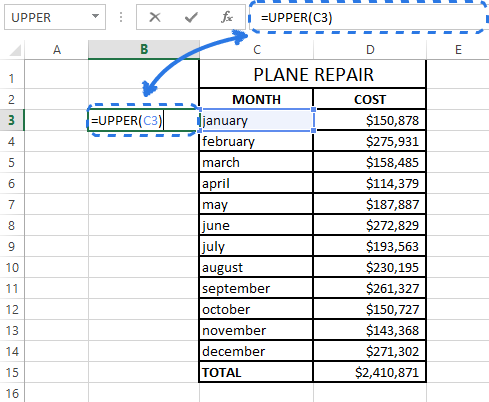
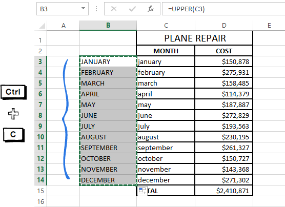
- Введите знак равенства (=) и имя функции UPPER (ПРОПИСН) в смежную ячейку нового столбца (B3).
- В скобках после имени функции введите соответствующую ссылку на ячейку (C3). Ваша формула должна выглядеть вот так:
=UPPER(C3)
=ПРОПИСН(C3)где C3 – это ячейка с текстом, который нужно преобразовать.
- Нажмите Enter.На рисунке выше видно, что в ячейке B3 содержится текст точно такой же, как в C3, только прописными буквами.
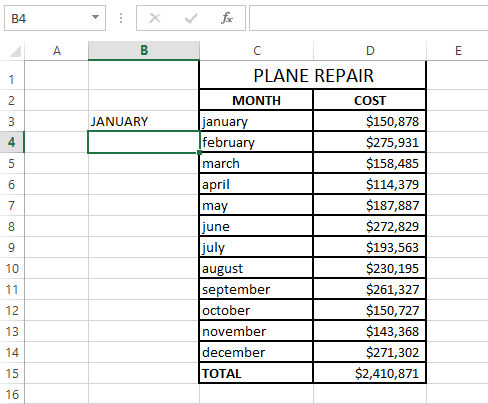 На рисунке выше видно, что в ячейке B3 содержится текст точно такой же, как в C3, только прописными буквами.
Копируем формулу вниз по столбцу
Теперь Вам нужно скопировать формулу в остальные ячейки вспомогательного столбца:
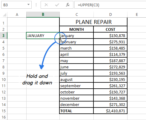
- Выделите ячейку с формулой.
- Наведите указатель мыши на маленький квадрат (маркер автозаполнения) в нижнем правом углу выделенной ячейки, чтобы указатель превратился в маленький черный крест.
- Нажмите и, удерживая левую кнопку мыши, протяните формулу вниз по всем ячейкам, в которые нужно её скопировать.
- Отпустите кнопку мыши.
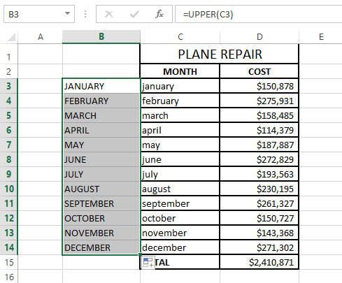
Замечание: Если Вам нужно полностью заполнить новый столбец (на всю высоту таблицы), то Вы можете пропустить шаги 5-7 и просто дважды кликнуть по маркеру автозаполнения.
Удаляем вспомогательный столбец
Итак, у Вас есть два столбца с одинаковыми текстовыми данными, отличающимися только регистром. Предполагаю, что Вы хотите оставить столбец только с нужным вариантом. Давайте скопируем значения из вспомогательного столбца и избавимся от него.
- Выделите ячейки, содержащие формулу, и нажмите Ctrl+C, чтобы скопировать их.
- Кликните правой кнопкой мыши по первой ячейке исходного столбца.
- В контекстном меню в разделе Paste Options (Параметры вставки) выберите Values (Значения).Поскольку нам нужны только текстовые значения, мы выберем именно этот вариант, чтобы в будущем избежать ошибок в формулах.
- Кликните правой кнопкой мыши по любой ячейке вспомогательного столбца и в контекстном меню выберите команду Delete (Удалить).
- В диалоговом окне Delete (Удаление ячеек) выберите вариант Entire column (Столбец) и нажмите ОК.
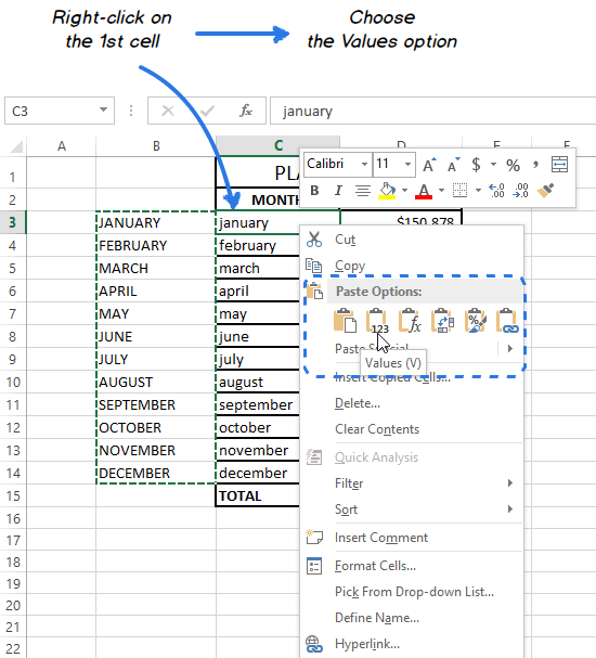 Поскольку нам нужны только текстовые значения, мы выберем именно этот вариант, чтобы в будущем избежать ошибок в формулах.
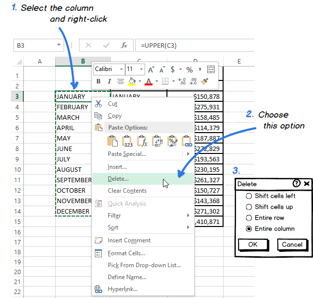
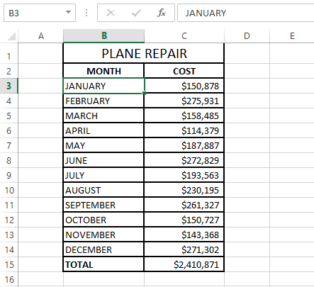
Готово!
В теории это может показаться слишком сложным. Расслабьтесь и попробуйте проделать все эти шаги самостоятельно. Вы увидите, что изменение регистра при помощи функций Excel – это совсем не трудно.
Изменяем регистр текста в Excel при помощи Microsoft Word
Если Вы не хотите возиться с формулами в Excel, Вы можете изменить регистр в Word. Далее Вы узнаете, как работает этот метод:
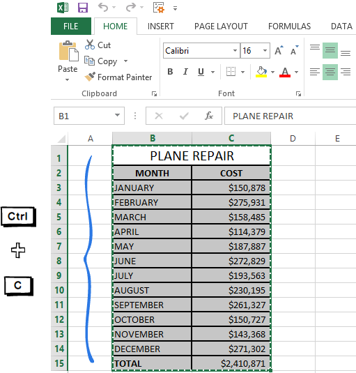
- Выделите диапазон на листе Excel, в котором необходимо изменить регистр текста.
- Нажмите Ctrl+C или кликните правой кнопкой мыши и в контекстном меню выберите команду Copy (Копировать).
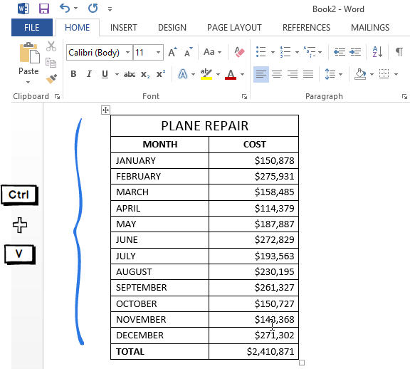
- Создайте новый документ Word.
- Нажмите Ctrl+V или щелкните правой кнопкой мыши по пустой странице и в контекстном меню выберите команду Paste (Вставить). Таблица Excel будет скопирована в Word.
- Выделите текст, у которого нужно изменить регистр.
- На вкладке Home (Главная) в разделе Font (Шрифт) нажмите иконку Change Case (Регистр).
- В раскрывающемся списке выберите один из 5 вариантов регистра.
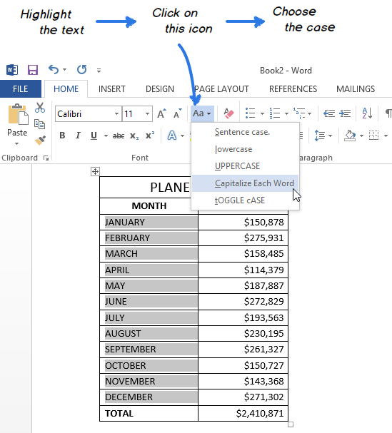
Замечание: Кроме этого, Вы можете нажимать сочетание Shift+F3, пока не будет установлен нужный стиль. При помощи этих клавиш можно выбрать только верхний и нижний регистр, а также регистр как в предложениях.
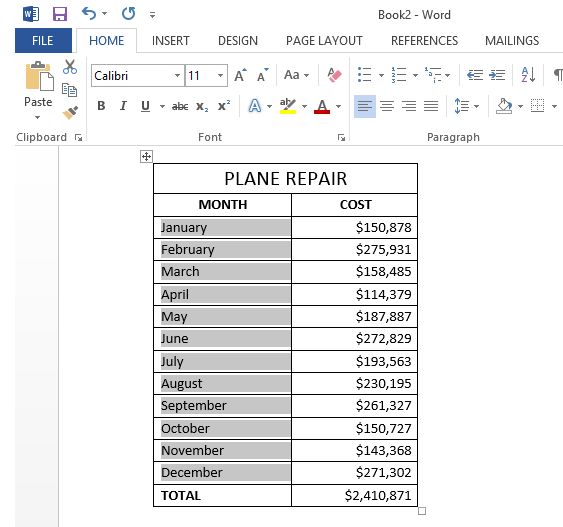
Теперь у Вас есть таблица в Word с изменённым регистром текста. Просто скопируйте её и вставьте на прежнее место в Excel.
Изменяем регистр текста при помощи макроса VBA
Вы также можете использовать макросы VBA в Excel 2010 и 2013. Не переживайте, если Ваши знания VBA оставляют желать лучшего. Какое-то время назад я тоже мало что знал об этом, а теперь могу поделиться тремя простыми макросами, которые изменяют регистр текста на верхний, нижний или делают каждое слово с прописной буквы.
Я не буду отвлекаться от темы и рассказывать Вам, как вставить и запустить код VBA в Excel, поскольку об этом замечательно рассказано в других статьях нашего сайта. Я просто покажу макросы, которые Вы можете скопировать и вставить в свою книгу.
- Если Вы хотите преобразовать текст в верхний регистр, используйте следующий макрос VBA:
Sub Uppercase()
    For Each Cell In Selection
        If Not Cell.HasFormula Then
            Cell.Value = UCase(Cell.Value)
        End If
    Next Cell
End Sub
- Чтобы применить нижний регистр к своим данным, используйте код, показанный ниже:
Sub Lowercase()
    For Each Cell In Selection
        If Not Cell.HasFormula Then
            Cell.Value = LCase(Cell.Value)
        End If
    Next Cell
End Sub
- Вот такой макрос сделает все слова в тексте, начинающимися с большой буквы:
Sub Propercase()
    For Each Cell In Selection
        If Not Cell.HasFormula Then
            Cell.Value = _
            Application _
            .WorksheetFunction _
            .Proper(Cell.Value)
        End If
    Next Cell
End Sub
Я надеюсь, что теперь, когда Вы знаете пару отличных приёмов изменения регистра в Excel, эта задача не вызовет у Вас затруднений. Функции Excel, Microsoft Word, макросы VBA – всегда к Вашим услугам. Вам осталось сделать совсем немного – определиться, какой из этих инструментов Вам больше нравится.
Оцените качество статьи. Нам важно ваше мнение:
Excel Change Case (Table of Contents)
- Introduction to Change Case in Excel
- How to Change Case in Excel?
Introduction to Change Case in Excel
As we know from childhood, we mostly use two kinds of cases: upper case and lower case. While we are working on a word document, it will warn us to adjust or will adjust in case if we wrongly give lowercase after a full stop or at the beginning of the statement, but this feature is not available in Excel. There are multiple ways to convert one case to another case in Excel and convert to correct the case.
How to Change Case in Excel?
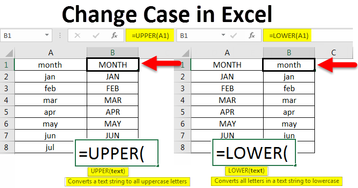
One way to convert the text from one case to another case is to use functions in excel. We have functions like “Upper,” “Lower,” and “Proper.” We will see one by one how to change cases in Excel and the impact of each because each one has its own features. First, let’s understand How to Change the Case in Excel with some examples.
You can download this Change Case Excel Template here – Change Case Excel Template
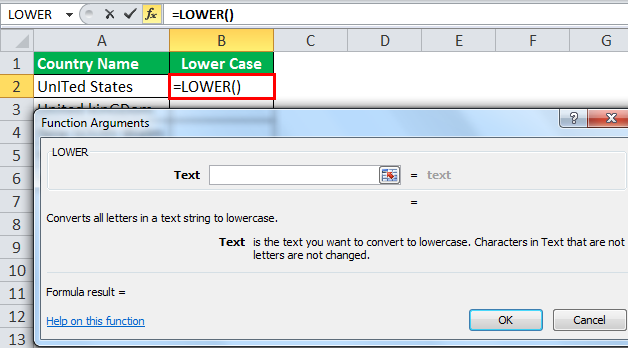
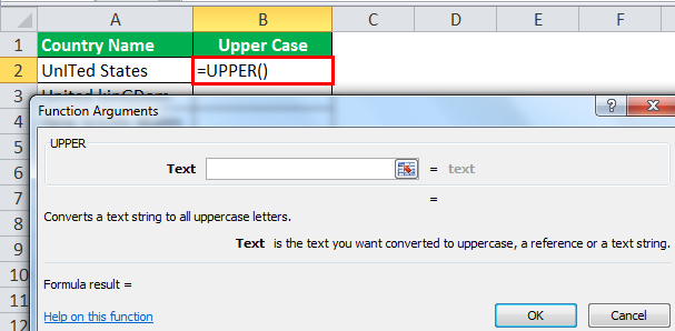
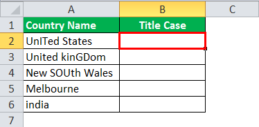
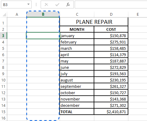
Example #1 – Change Case to Upper Case
This function helps to convert the text from any case to upper case. It is very easy to convert to upper case using this function. Try to input a small data table with all small cases.
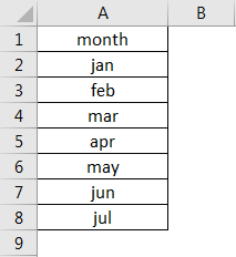
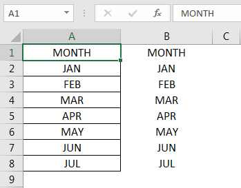
Observe the above screenshot; I have input January to July months in small case letters. Now our task is to convert them to upper case using the UPPER function. The data is in column A; hence input the function in column B.
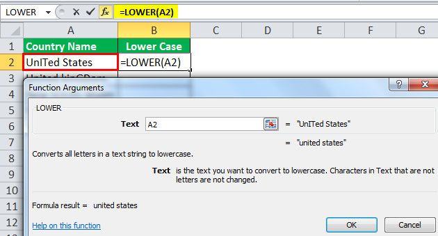
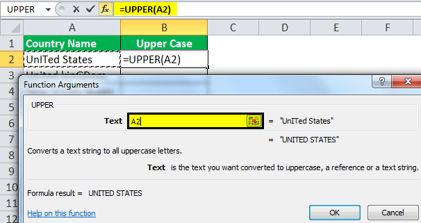
Syntax of the function is =UPPER(text). Observe the below screenshot for reference.
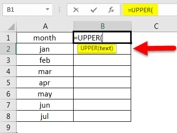
Here instead of text, give the cell address which we want to convert to uppercase. Here the cell address is A1.
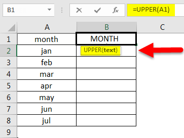
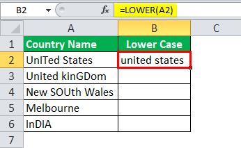
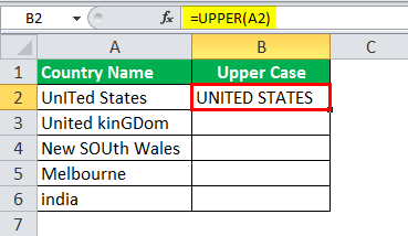
Observe the above screenshot, the month in cell A1 is converted into uppercase in B1. Now apply this to all other cells by dragging the formula until data is available or selecting the cell B1.
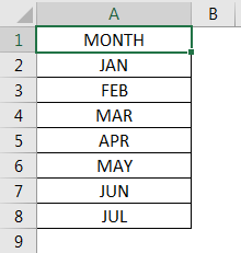
Then double click on the right bottom corner of the square.
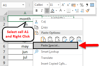
Now data is converted to Upper case, but it is not in the required place of a spreadsheet. So, copy the data that is converted in uppercase and select cell A1 and right click then, the below pop up menu will appear.
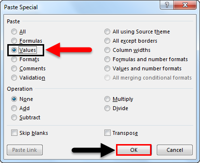
Choose the Paste Special option and select Values. Then click on OK.
Then the text will paste like below.
After deleting the column with formulas, we will get results as shown below.
Example #2 – Change Case to Lower Case
Up to now, we have seen how to convert small case to upper case. Now we will see how to convert an upper-case text into lower case text. This is also quite similar to the upper case function still; we will see one example of how to convert to lower case.
Consider the example which we already converted to upper case. Now we will convert the same months to lower case.
The syntax of lower is also similar to upper that is =LOWER(Text). Observe the below screenshot for reference.
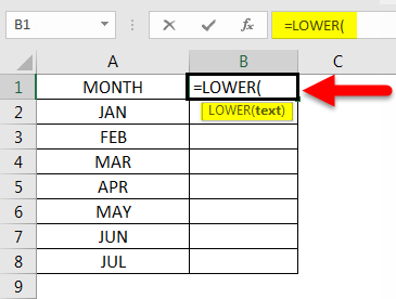
In place of text, we will input the Cell Address of text that we want to convert to lower. And press Enter. Then apply this to all other cells by dragging the formula until data is available.
As the text is converted to lower case, copy text and paste the data as similar to how we did in the upper case and delete the formula cells.
With this, we covered how to convert data a lower-case text to upper case and upper-case text to lower case. We have one more function called proper, which we have to discuss.
Example #3 – Change any case to a Proper Case
One more function is available to convert from one case to another case, but it is quite different from upper and lower functions. Because “UPPER” will convert everything to upper case and “LOWER” will convert everything to lower case, but “PROPER” will convert every first letter of the word to upper case and the remaining into lowercase.
Consider the below text, which is in a mixed-format; some letters are in the upper case and some lowercase letters. Now we will apply a proper function to these texts and will check how it converts.
The syntax for proper is similar as upper and lower =PROPER(text); find the below screenshot for reference.
Now select the cell address in place of text.
Now apply this to all other cells also by dragging the formula until data is available.
Observe text ‘J’ is capital in January ‘, I’ is capital in Is ‘F’ is capital in First ‘M’ is capital in Month. If we compare both texts, all the first letters of the word are uppercase.
Now we will see how it will convert if the entire text is in the upper case.
Even if all the texts are in the upper case, they will be converted in the same way. Hence it is not a concern what case we are using; whatever case, maybe it will convert into its own pattern (the first letter is the upper case in every word).
Up till now, we seen how to convert using function now will see how to change case with Flash fill in excel.
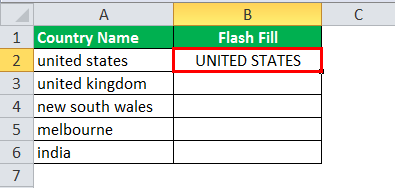
Example #4 – Flash Fill
Flash fill helps in a few cases when we want to convert the text into a particular pattern. Here we will discuss the names, but you can use this depending on the situation. Consider the below list of names.
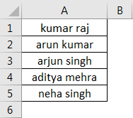
If we want only the first letter as upper case, give the next column pattern. Now select the next empty cell and select the option Flash Fill. Flash fill is available under the Data menu; please find the below screenshot for reference.
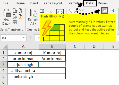
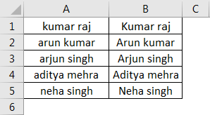
Once we click on the flash fill, it will fill the similar pattern as the above two names.
If we want to convert the first part of the name alone to the upper case, we have to use the combination of upper and left functions together.
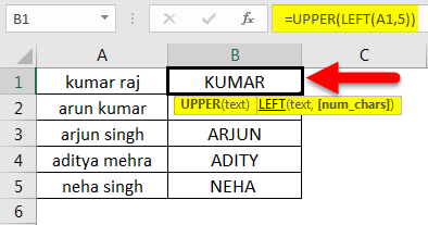
If we observe the formula, the result of a left function is “Kumar”, and the upper function converts that Kumar name to the upper case; hence the result is “KUMAR” similarly for the other cells too.
Things to Remember about Change Case in Excel
- Three functions help to convert the text from one case to another case.
- Upper converts any case text into upper case.
- Lower converts any case text into lower case.
- Proper convert any case text into a format of the first letter of the word will be upper case.
- If we want to take the help of a word document, we can copy the text from excel and paste the text into a word document and use the shortcut Shift + F3 to convert the text to upper, lower, and first letter upper formats. Now copy from word and paste it into excel.
Recommended Articles
This is a guide to Change Case in Excel. Here we discuss how to change case in excel along with practical examples and a downloadable excel template. You can also go through our other suggested articles –
- AVERAGE in Excel
- Count in Excel
- COUNTIF Function in Excel
- Excel MAX IF Function