
Look up values in a list of data
Excel for Microsoft 365 Excel for the web Excel 2021 Excel 2019 Excel 2016 Excel 2013 Excel 2010 Excel 2007 More…Less
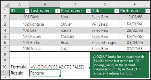
Let’s say that you want to look up an employee’s phone extension by using their badge number, or the correct rate of a commission for a sales amount. You look up data to quickly and efficiently find specific data in a list and to automatically verify that you are using correct data. After you look up the data, you can perform calculations or display results with the values returned. There are several ways to look up values in a list of data and to display the results.
What do you want to do?
-
Look up values vertically in a list by using an exact match
-
Look up values vertically in a list by using an approximate match
-
Look up values vertically in a list of unknown size by using an exact match
-
Look up values horizontally in a list by using an exact match
-
Look up values horizontally in a list by using an approximate match
-
Create a lookup formula with the Lookup Wizard (Excel 2007 only)
Look up values vertically in a list by using an exact match
To do this task, you can use the VLOOKUP function, or a combination of the INDEX and MATCH functions.
VLOOKUP examples

For more information, see VLOOKUP function.
INDEX and MATCH examples
In simple English it means:
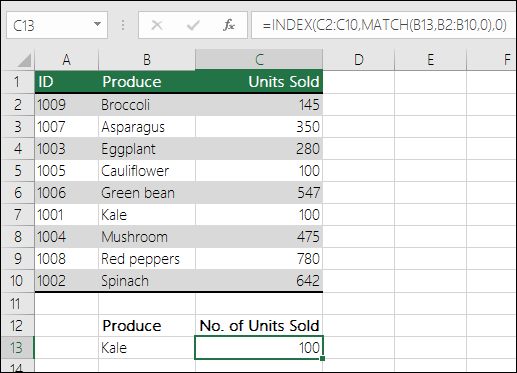
=INDEX(I want the return value from C2:C10, that will MATCH(Kale, which is somewhere in the B2:B10 array, where the return value is the first value corresponding to Kale))
The formula looks for the first value in C2:C10 that corresponds to Kale (in B7) and returns the value in C7 (100), which is the first value that matches Kale.
For more information, see INDEX function and MATCH function.
Top of Page
Look up values vertically in a list by using an approximate match
To do this, use the VLOOKUP function.
Important: Make sure the values in the first row have been sorted in an ascending order.
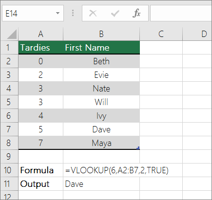
In the above example, VLOOKUP looks for the first name of the student who has 6 tardies in the A2:B7 range. There is no entry for 6 tardies in the table, so VLOOKUP looks for the next highest match lower than 6, and finds the value 5, associated to the first name Dave, and thus returns Dave.
For more information, see VLOOKUP function.
Top of Page
Look up values vertically in a list of unknown size by using an exact match
To do this task, use the OFFSET and MATCH functions.
Note: Use this approach when your data is in an external data range that you refresh each day. You know the price is in column B, but you don’t know how many rows of data the server will return, and the first column isn’t sorted alphabetically.
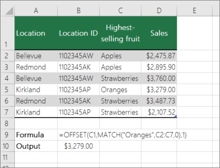
C1 is the upper left cells of the range (also called the starting cell).
MATCH(«Oranges»,C2:C7,0) looks for Oranges in the C2:C7 range. You should not include the starting cell in the range.
1 is the number of columns to the right of the starting cell where the return value should be from. In our example, the return value is from column D, Sales.
Top of Page
Look up values horizontally in a list by using an exact match
To do this task, use the HLOOKUP function. See an example below:
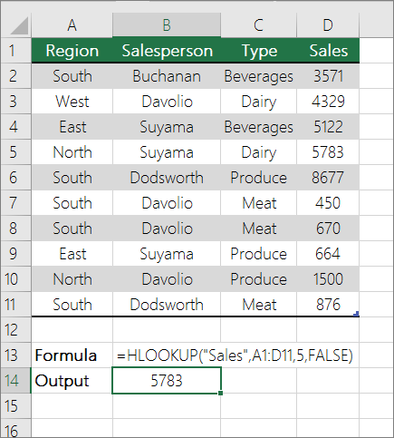
HLOOKUP looks up the Sales column, and returns the value from row 5 in the specified range.
For more information, see HLOOKUP function.
Top of Page
Look up values horizontally in a list by using an approximate match
To do this task, use the HLOOKUP function.
Important: Make sure the values in the first row have been sorted in an ascending order.
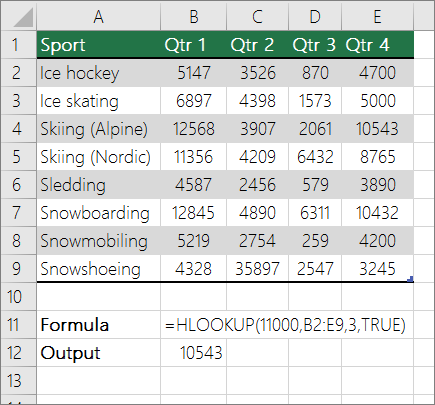
In the above example, HLOOKUP looks for the value 11000 in row 3 in the specified range. It does not find 11000 and hence looks for the next largest value less than 1100 and returns 10543.
For more information, see HLOOKUP function.
Top of Page
Create a lookup formula with the Lookup Wizard (Excel 2007 only)
Note: The Lookup Wizard add-in was discontinued in Excel 2010. This functionality has been replaced by the function wizard and the available Lookup and reference functions (reference).
In Excel 2007, the Lookup Wizard creates the lookup formula based on a worksheet data that has row and column labels. The Lookup Wizard helps you find other values in a row when you know the value in one column, and vice versa. The Lookup Wizard uses INDEX and MATCH in the formulas that it creates.
-
Click a cell in the range.
-
On the Formulas tab, in the Solutions group, click Lookup.
-
If the Lookup command is not available, then you need to load the Lookup Wizard add-in program.
How to load the Lookup Wizard Add-in program
-
Click the Microsoft Office Button
 , click Excel Options, and then click the Add-ins category.
 -
In the Manage box, click Excel Add-ins, and then click Go.
-
In the Add-Ins available dialog box, select the check box next to Lookup Wizard, and then click OK.
-
Follow the instructions in the wizard.
Top of Page
Need more help?
Table of Contents
- INTRODUCTION
- USE XLOOKUP IN EXCEL 2016,2013,2007,2019 OR ANY OTHER VERSION
- WHAT IS GKXLOOKUP ?
- WHEN TO USE GKXLOOKUP ?
- DOWNLOAD THE ADDIN FOR XLOOKUP IN EXCEL 2016,2019,2007,2010,2013
- INSTALLING THE XLOOKUP ADDIN [GKXLOOKUP]
- GKXLOOKUP: GENERAL INFORMATION
- GKXLOOKUP: EXAMPLE
- FAQs
- Is XLOOKUP available for Excel 2016?
- Is XLOOKUP available for Excel 2019?
- XLOOKUP is not working in my Excel.
- Is XLOOKUP case sensitive?
- Which Versions of Excel support XLOOKUP?
- Where can I find case sensitive XLOOKUP?
INTRODUCTION
XLOOKUP is a newly flavored lookup function provided in OFFICE 365.
The XLOOKUP is very much advanced and versatile when compared with the previous versions of lookup functions like
VLOOKUP , HLOOKUP or INDEX-MATCH etc.
XLOOKUP function lets us lookup in any column in the table whether it is to the extreme left of the lookup table or right or anywhere in the middle.It returns the value or the complete array at once as per the selection.Both of these functionalities were not available in the previous versions.
But, the biggest problem is that this function is not available for any of the versions except OFFICE 365 which means no version earlier to OFFICE 365 like Excel 2019, 2016, 2013,2010 or 2007 have this function.
So, Gyankosh.net created a version of this using VBA for our readers so that they don’t miss this opportunity for using this awesome function.
This article provides you an ADD IN and tells its usage which can be used in place of the XLOOKUP FUNCTION.
THE ADD-IN IS CREATED IN THE FORM OF A UTILITY FOR EASY USE.
USE XLOOKUP IN EXCEL 2016,2013,2007,2019 OR ANY OTHER VERSION
You can make use of Xlookup in Excel 2016, 2019 or any other version mentioned above using a custom function or any macro utility which is being discussed here.
Follow the article to get the free addin and use Xlookup in Excel 2016, 2019 or other versions.
WHAT IS GKXLOOKUP ?
GKXLOOKUP [ Gyankosh XLOOKUP] is a simple utility that acts like the XLOOKUP FUNCTION but it is available to all versions of EXCEL whether it is EXCEL 2019, or Excel 2016 or any previous versions.
WHEN TO USE GKXLOOKUP ?
The function [Utility] is very specifically meant for the situations such as:
- When you want to retrieve the information from a table by looking up any value and return a single value or a complete array. It gives CASE SENSITIVE INFORMATION such as two values differing only in the case. [ Easy and easy, cat and Cat and so on].
- Any column can be looked up and any column can be retrieved.
- Complete look up can be done in one go.
- Use this function when the built-in functions don’t work for you as VBA functions are a bit slower inherently.
DOWNLOAD THE ADDIN FOR XLOOKUP IN EXCEL 2016,2019,2007,2010,2013
ADDIN is like a small installation to your MICROSOFT EXCEL software which adds to the capabilities of the EXCEL.
CLICK ON THE BUTTON BELOW TO DOWNLOAD THE ADDIN FOR GKXLOOKUP FUNCTION and its executing macro.
Download both the files.
AFTER CLICKING THE BUTTON ABOVE, a file named gkxlookup_addin.xlam and gkxlookup_admin.xlam will ask your approval to save. Save both the files in the desired location.
SOMETIMES, DUE TO SETTINGS ISSUES IF THE BROWSER TRIES TO OPEN THIS FILE AND SHOW YOU ABSURD CHARACTERS, RIGHT-CLICK ON THE BUTTON>SAVE LINK AS>CHOOSE LOCATION AND SAVE THE FILE.
*DON'T WORRY ABOUT THE SECURITY WHEN DOWNLOADING AND INSTALLING THESE ADDINS . WE ARE A GROUP OF TECHNOLOGY ENTHUSIASTS AND HAVE CREATED THIS RESOURCE FOR HELPING OTHERS.
INSTALLING THE XLOOKUP ADDIN [GKXLOOKUP]
ADDIN is in the form of a simple excel file with a .xlam extension. Follow the steps to install the ADDIN in Excel.
THE FOLLOWING PROCESS OF INSTALLATION OF THE ADDIN IS BRIEF. IF YOU DON'T FIND IT COMFORTABLE USING THE BRIEF PROCESS, A COMPLETE DESCRIPTIVE PROCESS IS PRESENT HERE.
- OPEN EXCEL.
- Go to OPTIONS>ADDINS
- Select EXCEL ADD-INS
- Click GO.
- A new dialog box will open as shown in the picture containing all the EXCEL ADD-INS list.
- We can select the Addins we want to activate.
- In our case we want to install the add in , so click BROWSE.
- An OPEN FILE DIALOG BOX will open.
- Choose the ADD-IN file and click OK.
- The Add in will show in the list.
- Select it and click ok.
- Add in is installed.
For ADDING THE GKXLOOKUP TO TAB CLICK HERE. The process is shown in the picture below.

After adding the gkxlookup_addin.xlam Addin, repeat the process to add gkxlookup_admin.xlam in the same way.
GKXLOOKUP: GENERAL INFORMATION
As ARRAY functions are used using the CONTROL SHIFT ENTER, gyankosh.net created GKXLOOKUP in a simpler way in the form of a MACRO.
LET US UNDERSTAND THE STEPS TO USE THE GKXLOOKUP UTILITY.
STEP 1:
Create a button temporarily to assign the MACRO GKXLOOKUP or ADD IT IN A CUSTOM TAB for future use too.
For CREATING A BUTTON
- Go to DEVELOPER TAB.
- Click the Button option.
- Draw a button anywhere in the sheet.
- Right Click the button > Assign.
- The macro list will open.
- Choose GKXLOOKUP.
- Click OK.
For ADDING THE GKXLOOKUP TO TAB CLICK HERE.
STEP 2:
Select the cell where you want the result.
STEP 3:
Click the custom-created button or select the button from the new tab.

The field asks for the value or values to be looked up.

The following ways can be used to enter the value.
- Type the value in the field.
- Select all the values from the sheet itself directly and the range will be filled in the field given.
STEP 5:
After entering the LOOKUP VALUES, the next input field asks for the lookup array that is, the array from which we want to lookup the value.
We can select it on the sheet itself.
STEP 6:
The next option is select the Range for the return array or table. It can be a column or a range.

STEP 7:
The last option is to put the TEXT or MESSAGE which must be displayed if the values are not found.

GKXLOOKUP: EXAMPLE
FIND OUT THE VALUES AGAINST THE CODES FROM THE GIVEN TABLES.
Let us take the example of a coded language with the following codes.
We have two tables with some information about the different employees.
Table 1 contains the details like Employee id, employee name and employee location.
We got some additional information about the employees which is given in Table 2 shown below.
Table 2 contains additional employee details like Employee age and employee overtime.
We need to create a final table in which Table 1 contains all the information in a single table.
TABLE 1
| EMP ID | EMP NAME | EMP LOCATION |
| 1011 | DENIS | PARIS |
| 1021 | LEANDER | NEWYORK |
| 1030 | FRIDRICK | LONDON |
| 3021 | JOJO | PARIS |
| 4520 | JJ | LONDON |
| 8745 | KEVIN | PARIS |
| 6541 | CHUCK | DELHI |
| 3254 | CASPER | MOSCOW |
Few more information came through an email and contained the following table.
TABLE 2
| EMP ID | EMP AGE | OVERTIME |
| 1030 | 25 | 12 |
| 3021 | 23 | NA |
| 4520 | 26 | 13 |
| 8745 | 27 | 15 |
| 3254 | 29 | 17 |
| 6541 | 25 | NA |
| 1011 | 24 | 42 |
| 1021 | 25 | 12 |

STEPS TO SOLUTION
The first step to solve the problem is to create two more columns EMP AGE and OVERTIME in the first table i.e. TABLE 1 as shown in the picture below.

Enter the column name as EMP AGE and OVERTIME in the first table as shown in the picture above.
- Click the GKXLOOKUP UTILITY from the Gyankosh.net Tab. [ or any other name as per your choice ].
- The first input will be for the values to be looked up.
- Select the EMP ID COMPLETE COLUMN in the table 1 which we’ll be looking for in the Table 2.
- After selecting the lookup values, click ok.
- Second screen will be asking for LOOKUP ARRAY.
- Select EMP ID COLUMN FROM TABLE 2, the lookup array from which we need to fetch the values and click OK.
- The next value to be started is to select the RETURNING ARRAY.
- SELECT THE COMPLETE TABLE WHICH YOU WANT TO RETURN AGAINST THE LOOKED UP VALUES. For our values, select the columns EMP AGE and OVERTIME and click OK.
- The last value is the ERROR TEXT or value which will be placed if the value is not found.
- Click OK.
- The values will be looked up, fetched, and filled in the selected Cell in the same pattern as selected in the RETURN ARRAY OR TABLE.
FAQs
Is XLOOKUP available for Excel 2016?
No, XLOOKUP is not available for EXCEL 2016.
Is XLOOKUP available for Excel 2019?
No, XLOOKUP is not available for Excel 2019.
XLOOKUP is not working in my Excel.
XLOOKUP is not availble for all the versions of Excel but only Excel 365. You can use the utility discussed in this article to use XLOOKUP in other versions like EXCEL 2016, 2019 or others.
Is XLOOKUP case sensitive?
No Xlookup is not case sensitive. It’ll return all the matching cases.
Which Versions of Excel support XLOOKUP?
Only Excel 365 [ Excel for Office 365 ],supports built in Xlookup. No other version of Excel have XLOOKUP.
Where can I find case sensitive XLOOKUP?
The addin discussed in this article gives you case sensitive results. You can use that.
Содержание
- Поиск данных в таблице или диапазоне ячеек с помощью встроенных функций Excel
- Описание
- Создание образца листа
- Определения терминов
- Функции
- LOOKUP ()
- INDEX () и MATCH ()
- СМЕЩ () и MATCH ()
- Finding of the value in the column and the row of the Excel table
- Finding values in the Excel table
- Search of the value in the Excel ROW
- The principle of the formula for finding the value in the Excel ROW:
- How can I get to the column headings from a single cell value?
- Search the value in the Excel column
- The principle of the formula for finding the value in the Excel column
- Look up values in a list of data
- What do you want to do?
- Look up values vertically in a list by using an exact match
- VLOOKUP examples
- INDEX and MATCH examples
- Look up values vertically in a list by using an approximate match
- Look up values vertically in a list of unknown size by using an exact match
- Look up values horizontally in a list by using an exact match
- Look up values horizontally in a list by using an approximate match
- Create a lookup formula with the Lookup Wizard (Excel 2007 only)
Поиск данных в таблице или диапазоне ячеек с помощью встроенных функций Excel
Примечание: Мы стараемся как можно оперативнее обеспечивать вас актуальными справочными материалами на вашем языке. Эта страница переведена автоматически, поэтому ее текст может содержать неточности и грамматические ошибки. Для нас важно, чтобы эта статья была вам полезна. Просим вас уделить пару секунд и сообщить, помогла ли она вам, с помощью кнопок внизу страницы. Для удобства также приводим ссылку на оригинал (на английском языке).
Описание
В этой статье приведены пошаговые инструкции по поиску данных в таблице (или диапазоне ячеек) с помощью различных встроенных функций Microsoft Excel. Для получения одного и того же результата можно использовать разные формулы.
Создание образца листа
В этой статье используется образец листа для иллюстрации встроенных функций Excel. Рассматривайте пример ссылки на имя из столбца A и возвращает возраст этого человека из столбца C. Чтобы создать этот лист, введите указанные ниже данные в пустой лист Excel.
Введите значение, которое вы хотите найти, в ячейку E2. Вы можете ввести формулу в любую пустую ячейку на том же листе.
Определения терминов
В этой статье для описания встроенных функций Excel используются указанные ниже условия.
Вся таблица подстановки
Значение, которое будет найдено в первом столбце аргумента «инфо_таблица».
Просматриваемый_массив
-или-
Лукуп_вектор
Диапазон ячеек, которые содержат возможные значения подстановки.
Номер столбца в аргументе инфо_таблица, для которого должно быть возвращено совпадающее значение.
3 (третий столбец в инфо_таблица)
Ресулт_аррай
-или-
Ресулт_вектор
Диапазон, содержащий только одну строку или один столбец. Он должен быть такого же размера, что и просматриваемый_массив или Лукуп_вектор.
Логическое значение (истина или ложь). Если указано значение истина или опущено, возвращается приближенное соответствие. Если задано значение FALSE, оно будет искать точное совпадение.
Это ссылка, на основе которой вы хотите основать смещение. Топ_целл должен ссылаться на ячейку или диапазон смежных ячеек. В противном случае функция СМЕЩ возвращает #VALUE! значение ошибки #ИМЯ?.
Число столбцов, находящегося слева или справа от которых должна указываться верхняя левая ячейка результата. Например, значение «5» в качестве аргумента Оффсет_кол указывает на то, что верхняя левая ячейка ссылки состоит из пяти столбцов справа от ссылки. Оффсет_кол может быть положительным (то есть справа от начальной ссылки) или отрицательным (то есть слева от начальной ссылки).
Функции
LOOKUP ()
Функция Просмотр находит значение в одной строке или столбце и сопоставляет его со значением в той же позицией в другой строке или столбце.
Ниже приведен пример синтаксиса формулы подСТАНОВКи.
= Просмотр (искомое_значение; Лукуп_вектор; Ресулт_вектор)
Следующая формула находит возраст Марии на листе «образец».
= ПРОСМОТР (E2; A2: A5; C2: C5)
Формула использует значение «Мария» в ячейке E2 и находит слово «Мария» в векторе подстановки (столбец A). Формула затем соответствует значению в той же строке в векторе результатов (столбец C). Так как «Мария» находится в строке 4, функция Просмотр возвращает значение из строки 4 в столбце C (22).
Примечание. Для функции Просмотр необходимо, чтобы таблица была отсортирована.
Чтобы получить дополнительные сведения о функции Просмотр , щелкните следующий номер статьи базы знаний Майкрософт:
Функция ВПР или вертикальный просмотр используется, если данные указаны в столбцах. Эта функция выполняет поиск значения в левом столбце и сопоставляет его с данными в указанном столбце в той же строке. Функцию ВПР можно использовать для поиска данных в отсортированных или несортированных таблицах. В следующем примере используется таблица с несортированными данными.
Ниже приведен пример синтаксиса формулы ВПР :
= ВПР (искомое_значение; инфо_таблица; номер_столбца; интервальный_просмотр)
Следующая формула находит возраст Марии на листе «образец».
= ВПР (E2; A2: C5; 3; ЛОЖЬ)
Формула использует значение «Мария» в ячейке E2 и находит слово «Мария» в левом столбце (столбец A). Формула затем совпадет со значением в той же строке в Колумн_индекс. В этом примере используется «3» в качестве Колумн_индекс (столбец C). Так как «Мария» находится в строке 4, функция ВПР возвращает значение из строки 4 В столбце C (22).
Чтобы получить дополнительные сведения о функции ВПР , щелкните следующий номер статьи базы знаний Майкрософт:
INDEX () и MATCH ()
Вы можете использовать функции индекс и ПОИСКПОЗ вместе, чтобы получить те же результаты, что и при использовании поиска или функции ВПР.
Ниже приведен пример синтаксиса, объединяющего индекс и Match для получения одинаковых результатов поиска и ВПР в предыдущих примерах:
= Индекс (инфо_таблица; MATCH (искомое_значение; просматриваемый_массив; 0); номер_столбца)
Следующая формула находит возраст Марии на листе «образец».
= ИНДЕКС (A2: C5; MATCH (E2; A2: A5; 0); 3)
Формула использует значение «Мария» в ячейке E2 и находит слово «Мария» в столбце A. Затем он будет соответствовать значению в той же строке в столбце C. Так как «Мария» находится в строке 4, формула возвращает значение из строки 4 в столбце C (22).
Обратите внимание Если ни одна из ячеек в аргументе «число» не соответствует искомому значению («Мария»), эта формула будет возвращать #N/А.
Чтобы получить дополнительные сведения о функции индекс , щелкните следующий номер статьи базы знаний Майкрософт:
СМЕЩ () и MATCH ()
Функции СМЕЩ и ПОИСКПОЗ можно использовать вместе, чтобы получить те же результаты, что и функции в предыдущем примере.
Ниже приведен пример синтаксиса, объединяющего смещение и сопоставление для достижения того же результата, что и функция Просмотр и ВПР.
= СМЕЩЕНИЕ (топ_целл, MATCH (искомое_значение; просматриваемый_массив; 0); Оффсет_кол)
Эта формула находит возраст Марии на листе «образец».
= СМЕЩЕНИЕ (A1; MATCH (E2; A2: A5; 0); 2)
Формула использует значение «Мария» в ячейке E2 и находит слово «Мария» в столбце A. Формула затем соответствует значению в той же строке, но двум столбцам справа (столбец C). Так как «Мария» находится в столбце A, формула возвращает значение в строке 4 в столбце C (22).
Чтобы получить дополнительные сведения о функции СМЕЩ , щелкните следующий номер статьи базы знаний Майкрософт:
Источник
Finding of the value in the column and the row of the Excel table
We have the table in which the sales volumes of certain products are recorded in different months. It is necessary to find the data in the table, and the search criteria will be the headings of rows and columns. But the search must be performed separately by the range of the row or column. That is, only one of the criteria will be used. Therefore, you can`t apply the INDEX function here, but you need a special formula.
Finding values in the Excel table
To solve this problem, let us illustrate the example in the schematic table that corresponds to the conditions are described above.
The sheet with the table to search for values vertically and horizontally:
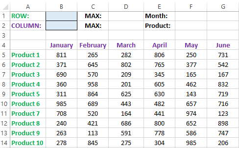
Above this table we can see the row with results. In the cell B1 we introduce the criterion for the search query, that is, the column header or the ROW name. And in the cell D1, to a search formula should return to the result of the calculation of the corresponding value. Then the second formula will work in the cell F1. She will already use the values of the cells B1 and D1 as the criteria for searching of the corresponding month.
Search of the value in the Excel ROW
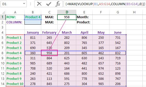
Now we are learning, in what maximum volume and in what month has been the maximum sale of the Product 4.
To search by columns:
- In the cell B1 you need to enter the value of the Product 4 — the name of the row, that will act as the criterion.
- In the cell D1 you need to enter the following:
- To confirm after entering the formula, you need to press the CTRL + SHIFT + Enter hotkey combination, because she must be executed in the array. If everything is done correctly, the curly braces will appear in the formula ROW.
- In the cell F1 you need to enter the second:
- For confirmation, to press the key combination CTRL + SHIFT + Enter again.
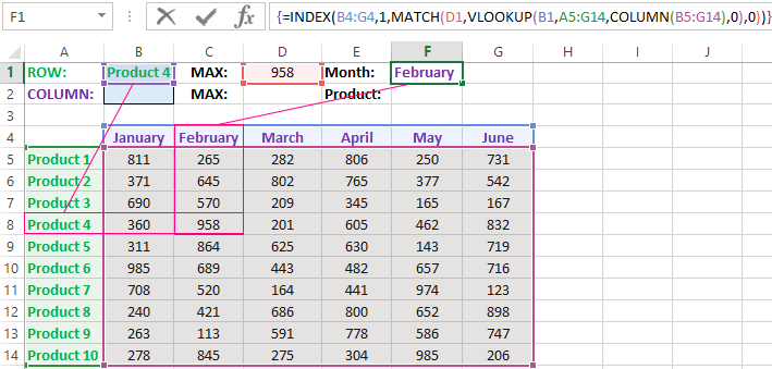
So we have found, in what month and what was the largest sale of the Product 4 for two quarters.
The principle of the formula for finding the value in the Excel ROW:
In the first argument of the VLOOKUP function (Vertical Look Up), indicates to the reference to the cell, where the search criterion is located. In the second argument indicates to the range of the cells for viewing during in the process of searching.
In the third argument of the VLOOKUP function should be indicated the number of the column from which you should to take the value against of the row named the Item 4. But since we do not previously know this number, we use the COLUMN function for creating the array of column numbers for the range B4:G15.
This allows the VLOOKUP function to collect the whole array of values. As a result, all relevant values are stored in memory for each column in the row Product 4 (namely: 360; 958; 201; 605; 462; 832). After that, the MAX function will only take the maximum number from this array and return it as the value for the cell D1, as the result of calculating.
As you can see, the construction of the formula is simple and concise. On its basis, it is possible in a similar way to find other indicators for a certain product. For example, the minimum or an average value of sales volume you need to find using for this purpose MIN or AVERAGE functions. Nothing hinders you from applying this skeleton of the formula to apply with more complex functions for implementation the most comfortable analysis of the sales report.
How can I get to the column headings from a single cell value?
For example, how effectively we displayed the month with the maximum sale, using of the second. It’s not difficult to notice that in the second formula we used the skeleton of the first formula without the MAX function. The main structure of the function is: VLOOKUP. We replaced the MAX on the MATCH, which in the first argument uses the value obtained by the previous formula. It acts as the criterion for searching for the month now.
And as a result, the MATCH function returns the column number 2, where the maximum value of the sales volume for the product is located for the product 4. After that, the INDEX function is included in the work. This function returns the value by the number of terms and column from the range specified in its arguments. Because the we have the number of column 2, and the row number in the range where the names of months are stored in any cases will be the value 1. Then we have the INDEX function to get the corresponding value from the range of B4:G4 — February (the second month).
Search the value in the Excel column
The second version of the task will be searching in the table with using the month name as the criterion. In such cases, we have to change the skeleton of our formula: the VLOOKUP function is replaced by the HLOOKUP (Horizontal Look Up) one, and the COLUMN function is replaced by the row one.
This will allow us to know what volume and what of the product the maximum sale was in a certain month.
To find what kind of the product had the maximum sales in a certain month, you should:
- In the cell B2 to enter the name of the month June — this value will be used as the search criterion.
- In the cell D2, you should to enter the formula:
- To confirm after entering the formula you need to press the combination of keys CTRL + SHIFT + Enter, as this formula will be executed in the array. And the curly braces will appear in the function ROW.
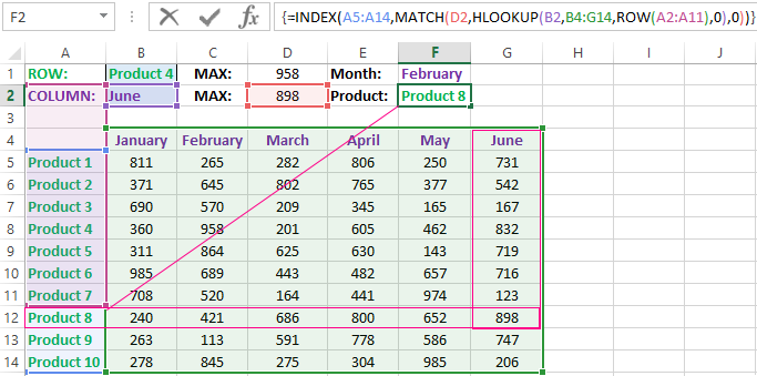
- In the cell F1, you need to enter the second:
- You need to click CTRL + SHIFT + Enter for confirmation again.
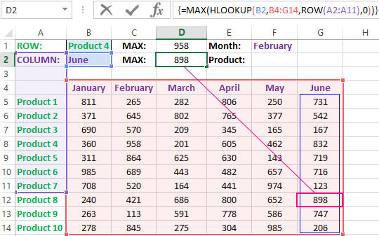
The principle of the formula for finding the value in the Excel column
In the first argument of the HLOOKUP function, we indicate to the reference by the cell with the criterion for the search. In the second argument specifies the reference to the table argument being scanned. The third argument is generated by the ROW function, what creates in the array of ROW numbers of 10 elements in memory. So there are 10 rows in the table section.
Further the HLOOKUP function, alternately using to each number of the row, creates the array of corresponding sales values from the table for the certain month (June). Further, the MAX function is left only to select the maximum value from this array.
Then just a little modifying to the first formula by using the INDEX and MATCH functions, we created the second function to display the names of the table rows according to the cell value. The names of the corresponding rows (products) we output in F2.
ATTENTION! When using the formula skeleton for other tasks, you need always to pay attention to the second and the third argument of the search HLOOKUP function. The number of covered rows in the range is specified in the argument, must match with the number of rows in the table. And also the numbering should begin with the second ROW!
Indeed, the content of the range generally we don’t care — we just need the row counter. That is, you need to change the arguments to: ROW(B2:B11) or ROW(C2:C11) — this does not affect in the quality of the formula. The main thing is that — there are 10 rows in these ranges, as well as in the table. And the numbering starts from the second row!
Источник
Look up values in a list of data
Let’s say that you want to look up an employee’s phone extension by using their badge number, or the correct rate of a commission for a sales amount. You look up data to quickly and efficiently find specific data in a list and to automatically verify that you are using correct data. After you look up the data, you can perform calculations or display results with the values returned. There are several ways to look up values in a list of data and to display the results.
What do you want to do?
Look up values vertically in a list by using an exact match
To do this task, you can use the VLOOKUP function, or a combination of the INDEX and MATCH functions.
VLOOKUP examples
For more information, see VLOOKUP function.
INDEX and MATCH examples
In simple English it means:
=INDEX(I want the return value from C2:C10, that will MATCH(Kale, which is somewhere in the B2:B10 array, where the return value is the first value corresponding to Kale))
The formula looks for the first value in C2:C10 that corresponds to Kale (in B7) and returns the value in C7 ( 100), which is the first value that matches Kale.
Look up values vertically in a list by using an approximate match
To do this, use the VLOOKUP function.
Important: Make sure the values in the first row have been sorted in an ascending order.
In the above example, VLOOKUP looks for the first name of the student who has 6 tardies in the A2:B7 range. There is no entry for 6 tardies in the table, so VLOOKUP looks for the next highest match lower than 6, and finds the value 5, associated to the first name Dave, and thus returns Dave.
For more information, see VLOOKUP function.
Look up values vertically in a list of unknown size by using an exact match
To do this task, use the OFFSET and MATCH functions.
Note: Use this approach when your data is in an external data range that you refresh each day. You know the price is in column B, but you don’t know how many rows of data the server will return, and the first column isn’t sorted alphabetically.
C1 is the upper left cells of the range (also called the starting cell).
MATCH(«Oranges»,C2:C7,0) looks for Oranges in the C2:C7 range. You should not include the starting cell in the range.
1 is the number of columns to the right of the starting cell where the return value should be from. In our example, the return value is from column D, Sales.
Look up values horizontally in a list by using an exact match
To do this task, use the HLOOKUP function. See an example below:
HLOOKUP looks up the Sales column, and returns the value from row 5 in the specified range.
For more information, see HLOOKUP function.
Look up values horizontally in a list by using an approximate match
To do this task, use the HLOOKUP function.
Important: Make sure the values in the first row have been sorted in an ascending order.
In the above example, HLOOKUP looks for the value 11000 in row 3 in the specified range. It does not find 11000 and hence looks for the next largest value less than 1100 and returns 10543.
For more information, see HLOOKUP function.
Create a lookup formula with the Lookup Wizard (Excel 2007 only)
Note: The Lookup Wizard add-in was discontinued in Excel 2010. This functionality has been replaced by the function wizard and the available Lookup and reference functions (reference).
In Excel 2007, the Lookup Wizard creates the lookup formula based on a worksheet data that has row and column labels. The Lookup Wizard helps you find other values in a row when you know the value in one column, and vice versa. The Lookup Wizard uses INDEX and MATCH in the formulas that it creates.
Click a cell in the range.
On the Formulas tab, in the Solutions group, click Lookup.
If the Lookup command is not available, then you need to load the Lookup Wizard add-in program.
How to load the Lookup Wizard Add-in program
Click the Microsoft Office Button  , click Excel Options, and then click the Add-ins category.
In the Manage box, click Excel Add-ins, and then click Go.
In the Add-Ins available dialog box, select the check box next to Lookup Wizard, and then click OK.
Источник

Программа предназначена для сравнения и подстановки значений в таблицах Excel.
Если вам надо сравнить 2 таблицы (по одному столбцу, или по нескольким),
и для совпадающих строк скопировать значения выбранных столбцов из одной таблицы в другую,
надстройка «Lookup» поможет сделать это нажатием одной кнопки.
То же самое можно сделать при помощи формулы =ВПР(), но:
- формулы могут тормозить работу с файлом при пересчёте, если объём данных большой (много строк или столбцов)
- если источник данных или файл, в который подставляются данные, каждый раз новый, — требуется время на прописывание или редактирование формул
- если с файлами работают люди, «далёкие» от Excel, — их проще обучить нажимать одну кнопку, чем объяснять им, как прописывать эти формулы
- иногда нужны дополнительные возможности (не учитывать заданные слова и символы при сравнении, выделять цветом изменения, копировать недостающие строки, и т.д.)
В настройках программы можно задать:
- где искать сравниваемые файлы (использовать уже открытый файл, загружать файл по заданному пути, или же выводить диалоговое окно выбора файла)
- с каких листов брать данные (варианты: активный лист, лист с заданным номером или названием)
- какие столбцы сравнивать (можно задать несколько столбцов)
- значения каких столбцов надо копировать в найденные строки (также можно указать несколько столбцов)
- каким цветом подсвечивать совпавшие и ненайденные строки (для каждого из 2 файлов)
- исключаемые при сравнении символы и фразы
Справка по надстройке Lookup
This Excel tutorial explains how to use the Excel LOOKUP function with syntax and examples.
Description
The Microsoft Excel LOOKUP function returns a value from a range (one row or one column) or from an array.
The LOOKUP function is a built-in function in Excel that is categorized as a Lookup/Reference Function. It can be used as a worksheet function (WS) in Excel. As a worksheet function, the LOOKUP function can be entered as part of a formula in a cell of a worksheet.
There are 2 different syntaxes for the LOOKUP function:
LOOKUP Function (Syntax #1)
In Syntax #1, the LOOKUP function searches for value in the lookup_range and returns the value in the result_range that is in the same position.
The syntax for the LOOKUP function in Microsoft Excel is:
LOOKUP( value, lookup_range, [result_range] )
Parameters or Arguments
- value
- The value to search for in the lookup_range.
- lookup_range
- A single row or single column of data that is sorted in ascending order. The LOOKUP function searches for value in this range.
- result_range
- Optional. It is a single row or single column of data that is the same size as the lookup_range. The LOOKUP function searches for the value in the lookup_range and returns the value from the same position in the result_range. If this parameter is omitted, it will return the first column of data.
Returns
The LOOKUP function returns any datatype such as a string, numeric, date, etc.
If the LOOKUP function can not find an exact match, it chooses the largest value in the lookup_range that is less than or equal to the value.
If the value is smaller than all of the values in the lookup_range, then the LOOKUP function will return #N/A.
If the values in the LOOKUP_range are not sorted in ascending order, the LOOKUP function will return the incorrect value.
Example (as Worksheet Function)
Let’s look at some Excel LOOKUP function examples and explore how to use the LOOKUP function as a worksheet function in Microsoft Excel:
Based on the Excel spreadsheet above, the following LOOKUP examples would return:
=LOOKUP(10251, A1:A6, B1:B6)
Result: "Pears"

=LOOKUP(10251, A1:A6)
Result: 10251

=LOOKUP(10246, A1:A6, B1:B6)
Result: #N/A

=LOOKUP(10248, A1:A6, B1:B6)
Result: "Apples"
LOOKUP Function (Syntax #2)
In Syntax #2, the LOOKUP function searches for the value in the first row or column of the array and returns the corresponding value in the last row or column of the array.
The syntax for the LOOKUP function in Microsoft Excel is:
LOOKUP( value, array )
Parameters or Arguments
- value
- The value to search for in the array. The values must be in ascending order.
- array
- An array of values that contains both the values to search for and return.
Returns
The LOOKUP function returns any datatype such as a string, numeric, date, etc.
If the LOOKUP function can not find an exact match, it chooses the largest value in the lookup_range that is less than or equal to the value.
If the value is smaller than all of the values in the lookup_range, then the LOOKUP function will return #N/A.
If the values in the array are not sorted in ascending order, the LOOKUP function will return the incorrect value.
Example (as Worksheet Function)
Let’s look at some Excel LOOKUP function examples and explore how to use the LOOKUP function as a worksheet function in Microsoft Excel:
=LOOKUP("T", {"s","t","u","v";10,11,12,13})
Result: 11

=LOOKUP("Tech on the Net", {"s","t","u","v";10,11,12,13})
Result: 11

=LOOKUP("t", {"s","t","u","v";"a","b","c","d"})
Result: "b"

=LOOKUP("r", {"s","t","u","v";"a","b","c","d"})
Result: #N/A

=LOOKUP(2, {1,2,3,4;511,512,513,514})
Result: 512
Frequently Asked Questions
Question: In Microsoft Excel, I have a table of data in cells A2:D5. I’ve tried to create a simple LOOKUP to find CB2 in the data, but it always returns 0. What am I doing wrong?
Answer: Using the LOOKUP function can sometimes be a bit tricky so let’s look at an example. Below we have a spreadsheet with the data that you described.
In cell F1, we’ve placed the following formula:
=LOOKUP("CB2",A2:A5,D2:D5)
And yes, even though CB2 exists in the data, the LOOKUP function returns 0.
Now, let’s explain what is happening. At first, it looks like the function isn’t finding CB2 in the list, but in fact, it is finding something else. Let’s fill in the empty cells in D3:D5 to explain better.
If we place the values TEST1, TEST2, TEST3 in cells D3, D4, 5, respectively, we can see that the LOOKUP function is in fact returning the value TEST2. So we ask ourselves, when we are looking up CB2 in the data and CB2 exists in the data, why is it returning the value for CB19? Good question. The LOOKUP function assumes that the data in column A is sorted in ascending order.
If you look closer at column A, it is not in fact sorted in ascending order. If we quickly sorted column A, it would look like this:
Now the LOOKUP function correctly returns 3A when it is looking up CB2 in the data.
To avoid these sorting problems with your data, we recommend using VLOOKUP function in this case. Let’s show you how we would do this. If we changed our formula below (but left our data in column A in the original sort order):
The following VLOOKUP formula would return the correct value of 3A.
=VLOOKUP("CB2",$A$2:$D$5,4,FALSE)
The VLOOKUP function does not require us to have the data sorted in ascending order since we used FALSE as the last parameter — which means that it is looking for an exact match.
Question: I have the following LOOKUP formula:
=LOOKUP(C2,{"A","B","C","D","E","F","G","H","I","K","X","Z"}, {"1","2","3","4","5","6","7","8","9","10","12","1"})
I also need to add zero to the lookup vector and result vector. How do I do this?
Answer: Using numbers in Excel can be tricky, as you can enter them either as numeric or text values. Because of this, there are 2 possible solutions.
Numeric Solution
If you have entered your zero as a numeric value, then the following formula will work:
=LOOKUP(C2,{0,"A","B","C","D","E","F","G","H","I","K","X","Z"}, {0,"1","2","3","4","5","6","7","8","9","10","12","1"})
Text Solution
If you have entered your zero as a text value, then the following formula will work:
=LOOKUP(C2,{"0","A","B","C","D","E","F","G","H","I","K","X","Z"}, {"0","1","2","3","4","5","6","7","8","9","10","12","1"})
Question: For the following function in Microsoft Excel:
=LOOKUP(M14,Sheet2!A2:A2240,Sheet2!B2:B2240)
How do I get it to return a blank cell if the LOOKUP value (M14) is blank?
Answer: To check for a blank value in cell M14, you can use the IF function and ISBLANK function as follows:
=IF(ISBLANK(M14),"",LOOKUP(M14,Sheet2!A2:A2240,Sheet2!B2:B2240))
Now if the value in cell M14 is blank, the formula will return a blank. Otherwise it will perform the LOOKUP function as before.