
Use LOOKUP, one of the lookup and reference functions, when you need to look in a single row or column and find a value from the same position in a second row or column.
For example, let’s say you know the part number for an auto part, but you don’t know the price. You can use the LOOKUP function to return the price in cell H2 when you enter the auto part number in cell H1.
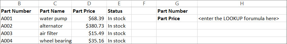
Use the LOOKUP function to search one row or one column. In the above example, we’re searching prices in column D.
Tips: Consider one of the newer lookup functions, depending on which version you are using.
-
Use VLOOKUP to search one row or column, or to search multiple rows and columns (like a table). It’s a much improved version of LOOKUP. Watch this video about how to use VLOOKUP.
-
If you are using Microsoft 365, use XLOOKUP — it’s not only faster, it also lets you search in any direction (up, down, left, right).
There are two ways to use LOOKUP: Vector form and Array form
-
Vector form: Use this form of LOOKUP to search one row or one column for a value. Use the vector form when you want to specify the range that contains the values that you want to match. For example, if you want to search for a value in column A, down to row 6.

-
Array form: We strongly recommend using VLOOKUP or HLOOKUP instead of the array form. Watch this video about using VLOOKUP. The array form is provided for compatibility with other spreadsheet programs, but it’s functionality is limited.
An array is a collection of values in rows and columns (like a table) that you want to search. For example, if you want to search columns A and B, down to row 6. LOOKUP will return the nearest match. To use the array form, your data must be sorted.
Vector form
The vector form of LOOKUP looks in a one-row or one-column range (known as a vector) for a value and returns a value from the same position in a second one-row or one-column range.
Syntax
LOOKUP(lookup_value, lookup_vector, [result_vector])
The LOOKUP function vector form syntax has the following arguments:
-
lookup_value Required. A value that LOOKUP searches for in the first vector. Lookup_value can be a number, text, a logical value, or a name or reference that refers to a value.
-
lookup_vector Required. A range that contains only one row or one column. The values in lookup_vector can be text, numbers, or logical values.
Important: The values in lookup_vector must be placed in ascending order: …, -2, -1, 0, 1, 2, …, A-Z, FALSE, TRUE; otherwise, LOOKUP might not return the correct value. Uppercase and lowercase text are equivalent.
-
result_vector Optional. A range that contains only one row or column. The result_vector argument must be the same size as lookup_vector. It has to be the same size.
Remarks
-
If the LOOKUP function can’t find the lookup_value, the function matches the largest value in lookup_vector that is less than or equal to lookup_value.
-
If lookup_value is smaller than the smallest value in lookup_vector, LOOKUP returns the #N/A error value.
Vector examples
You can try out these examples in your own Excel worksheet to learn how the LOOKUP function works. In the first example, you’re going to end up with a spreadsheet that looks similar to this one:
-
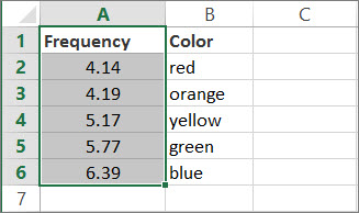
Copy the data in following table, and paste it into a new Excel worksheet.
Copy this data into column A
Copy this data into column B
Frequency
4.14
Color
red
4.19
orange
5.17
yellow
5.77
green
6.39
blue
-
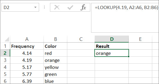
Next, copy the LOOKUP formulas from the following table into column D of your worksheet.
Copy this formula into the D column
Here’s what this formula does
Here’s the result you’ll see
Formula
=LOOKUP(4.19, A2:A6, B2:B6)
Looks up 4.19 in column A, and returns the value from column B that is in the same row.
orange
=LOOKUP(5.75, A2:A6, B2:B6)
Looks up 5.75 in column A, matches the nearest smaller value (5.17), and returns the value from column B that is in the same row.
yellow
=LOOKUP(7.66, A2:A6, B2:B6)
Looks up 7.66 in column A, matches the nearest smaller value (6.39), and returns the value from column B that is in the same row.
blue
=LOOKUP(0, A2:A6, B2:B6)
Looks up 0 in column A, and returns an error because 0 is less than the smallest value (4.14) in column A.
#N/A
-
For these formulas to show results, you may need to select them in your Excel worksheet, press F2, and then press Enter. If you need to, adjust the column widths to see all the data.
Array form
The array form of LOOKUP looks in the first row or column of an array for the specified value and returns a value from the same position in the last row or column of the array. Use this form of LOOKUP when the values that you want to match are in the first row or column of the array.
Syntax
LOOKUP(lookup_value, array)
The LOOKUP function array form syntax has these arguments:
-
lookup_value Required. A value that LOOKUP searches for in an array. The lookup_value argument can be a number, text, a logical value, or a name or reference that refers to a value.
-
If LOOKUP can’t find the value of lookup_value, it uses the largest value in the array that is less than or equal to lookup_value.
-
If the value of lookup_value is smaller than the smallest value in the first row or column (depending on the array dimensions), LOOKUP returns the #N/A error value.
-
-
array Required. A range of cells that contains text, numbers, or logical values that you want to compare with lookup_value.
The array form of LOOKUP is very similar to the HLOOKUP and VLOOKUP functions. The difference is that HLOOKUP searches for the value of lookup_value in the first row, VLOOKUP searches in the first column, and LOOKUP searches according to the dimensions of array.
-
If array covers an area that is wider than it is tall (more columns than rows), LOOKUP searches for the value of lookup_value in the first row.
-
If an array is square or is taller than it is wide (more rows than columns), LOOKUP searches in the first column.
-
With the HLOOKUP and VLOOKUP functions, you can index down or across, but LOOKUP always selects the last value in the row or column.
Important: The values in array must be placed in ascending order: …, -2, -1, 0, 1, 2, …, A-Z, FALSE, TRUE; otherwise, LOOKUP might not return the correct value. Uppercase and lowercase text are equivalent.
-
We all know the famous star of Excel functions VLOOKUP. It is commonly used for looking up values with a unique Id. But this is not the only function that can be used for looking up values in Excel. There are many other functions and formulas that can be used to lookup value. In this article, I will introduce you with all these Excel lookup functions and formulas. Some are even better than the VLOOKUP function in Excel. So, read to the end.
1. The Excel VLOOKUP Function
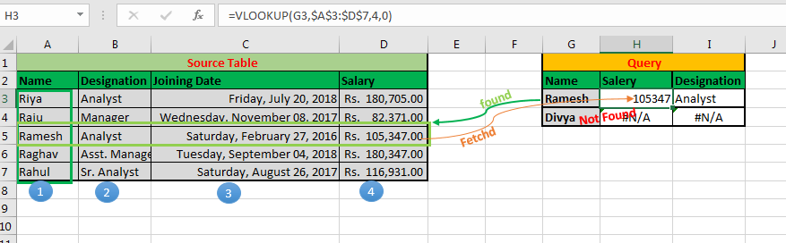
The first excel lookup function is of course the VLOOKUP function. This function is famous for a reason. We can use this function to do more than just a lookup. But the basic task of this function is to lookup values in the table, from left to right.
Syntax of VLOOKUP function:
=VLOOKUP(lookup_value, table_array, col_index_number, [range_lookup])
Lookup_value: The value by which you want to search in the first column of Table Array.
Table_array: The Table in which you want to look up/search
col_index_number: The column number in Table Array from which you want to fetch results.
[range_lookup]: FALSE if you want to search for exact value, TRUE if you want an approximate match.
Advantages of VLOOKUP:
- Easy to use.
- Fast
- Multiple Use
- Best for looking up values in vertical order.
Disadvantages:
- It is only used for Vertical Lookup
- It returns only the first matched value.
- Static until used with MATCH function.
- Can’t lookup values from the left of the lookup value.
You can read about this Excel Lookup Formula in detail here.
2. The Excel HLOOKUP Function
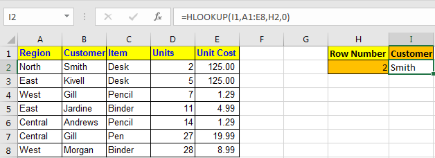
The HLOOKUP function is the missing part of the VLOOKUP function. The HLOOKUP function is used to lookup values horizontally. In other words, when you want to lookup a value in Excel by matching value in columns and get values from rows, then we use the HLOOKUP function. This is exactly the apposite of the VLOOKUP function.
Syntax of HLOOKUP
=HLOOKUP(lookup value, table array, row index number, [range_lookup] )
- lookup value : The value you are looking for.
- Table Array : The table in which you are looking for the value.
- Row Index Number : The row number in the Table from which you want retrieve data.
- [range_lookup] : its the match type. 0 for the exact match and 1 for approximate match.
Advantages of HLOOKUP Function:
- It can lookup values horizontally.
- Easy to use.
- Multiple Use
- Fast
Disadvantages:
- It is only used for Horizontal Lookup
- It returns only the first matched value.
- Static until used with the MATCH function.
- Can’t lookup values above the lookup values in the table.
You can learn about this Excel lookup function here.
3. The INDEX-MATCH Lookup Formula
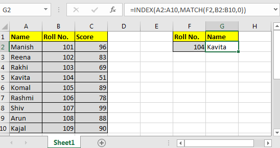
Where VLOOKUP and HLOOKUP can’t reach, this formula can reach. This is the best lookup formula in Excel till Excel 2016 (XLOOKUP is on the way).
The Generic Formula of INDEX MATCH
=INDEX (Result_Range,MATCH(lookup_value,lookup range,0))
Result_Range: It is the range range from where you want to retrieve value.
Lookup_value: It is the value that you want to match.
Lookup_Range: It is range in which you want to match the lookup value.
Advantages of INDEX-MATCH lookup formula:
- Can lookup in four directions. It can lookup values to the left and up of the lookup value.
- Dynamic.
- No need to define the row or column index.
Disadvantages:
- It may be difficult for new users.
- Uses two Excel functions in combination. Users need to understand the working of the INDEX and MATCH function.
You can learn about this formula here.
4: Excel OFFSET-MATCH Lookup Formula
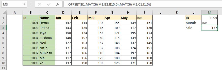
This is another formula that can be used to lookup values dynamically. This excel lookup formula uses the OFFSET function as anchor function and MATCH as a feeder function. Using this formula, we can dynamically retrieve values from a table by looking up in rows and columns.
Generic Formula,
=OFFSET(StartCell,MATCH(RowLookupValue,RowLookupRange,0),MATCH(ColLookupValue,ColLookupRange,0))
StartCell: This is the starting cell of lookup Table. Let’s say if you want to lookup in range A2:A10, then the StartCell will be A1.
RowLookupValue: This is the lookup value that you want to find in rows below the StartCell.
RowLookupRange: This is the range in which you want to lookup the RowLookupValue. It is the range below StartCell (A2:A10).
ColLookupValue: This is the lookup value that you want to find in columns (headers).
ColLookupRange: This is the range in which you want to lookup the ColLookupValue. It is the range on the right hand side of StartCell (like B1:D1).
Advantages of this Excel lookup technique:
- Fast
- Can lookup horizontally and vertically.
- Dynamic
Disadvantages:
- Complex to some people.
- Need to understand the working of OFFSET function and MATCH function.
You can learn about this lookup formula here in detail.
5: Excel LOOKUP Formula Multiple Values
All of the above lookup formulas return the first found value from the array. If there are more than one match they will not return other matches. In that case, this formula comes into action to save the day. This formula returns all the matched values from the list, instead of the first match only.
This formula use INDEX, ROW, and IF functions as main functions. The IFERROR function can be used optionally to handle errors.
Generic Formula
{=INDEX(array,SMALL(IF(lookup_value=lookup_value_range,ROW(lookup_value_range)-ROW(first cell of lookup_value_range)+1),ROW(1:1)))}
Array: The range from where you want to fetch data.
lookup_value: Your lookup_value that you want to filter.
lookup_value_range: The range in which you want to filter lookup_value.
The first cell in lookup_value range: if your lookup_value range is $A$5:$A$100 then its $A$5.
Important: Everything should be absolute referenced. lookup_value can be relative according to requirement.
Enter it as an array formula. After writing formula hit CTRL+SHIFT+ENTER key to make it an array formula.
As you can see in the gif, it returns all the matches from the excel table.
Advantages:
- Returns with multiple matched values from the Excel Table.
- Dynamic
Disadvantages:
- It’s too complex for a new user to understand.
- Uses array formula
- Need to define the possible number of outputs and apply this formula as a multi-cell array formula (Not in Excel 2019 and 365).
- Slow.
You can learn about this formula here in detail.
6: VLOOKUP-CHOOSE Lookup Excel Formula
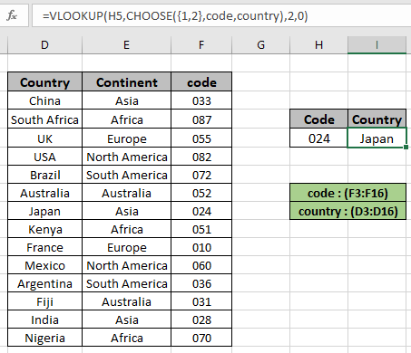 So, most people say that it is not possible to lookup values from the left of the lookup value in Excel using VLOOKUP function. Well, I am sorry to say, but they are wrong. We can lookup to the left of the lookup value in Excel using VLOOKUP function with the help of the CHOOSE function.
Generic Formula:
= VLOOKUP ( lookup_value , CHOOSE ( { 1 , 2 } , lookup_range , req_range ) , 2 , 0)
lookup_value : value to look for
lookup_range : range, where to look lookup_value
req_range : range, where corresponding value is required
2 : second column, num representing the req_range
0 : look for the exact match
In this formula, we basically create a virtual table inside the formula using the CHOOSE function. The CHOOSE function creates a table of two columns. The first column contains the lookup range and the second column contains the result range.
Advantages of VLOOKUP-CHOOSE lookup formula:
- You can lookup to the left of lookup value
- Fast
- Easy
Disadvantages:
- The CHOOSE function is rarely used. Users need to understand its working.
You can learn about this lookup formula here.
So yeah guys, these are the different lookup functions and formulas. That is not all. There can be many more lookup formulas in Excel that can be created using different combinations of Excel formulas. If you have any special lookup techniques, please share in the comments section below. We will include it in our article with your name.
I hope it was helpful and informative. If you have any doubts regarding this article, ask me in the comments section below.
Related Articles:
10+ New Functions in Excel 2019 and 365: Although the functions available in Excel 2016 and older are enough to work out any kind of calculation and automation, sometimes the formulas get tricky. These kinds of minor but important things are solved in Excel 2019 and 365.
17 Things About Excel VLOOKUP: The VLOOKUP is just not a lookup formula, it is more than that. The VLOOKUP has many other abilities and can be used for multiple purposes. In this article, we explore all the possible uses of VLOOKUP function.
10+ Creative Advanced Excel Charts to Rock Your Dashboard: Excel is a powerful data visualization tool that can be used to create stunning charts in Excel. These 15 advanced excel charts can be used to mesmerize your colleagues and bosses.
4 Creative Target Vs Achievement Charts in Excel: The target vs achievement charts are the most basic and important charts in any business. So it is better to put them most creative way possible. These 4 creative charts can make your dashboards rock the presentation.
Popular Articles:
50 Excel Shortcuts to Increase Your Productivity | Get faster at your task. These 50 shortcuts will make you work even faster on Excel.
How to use Excel VLOOKUP Function| This is one of the most used and popular functions of excel that is used to lookup value from different ranges and sheets.
How to use the Excel COUNTIF Function| Count values with conditions using this amazing function. You don’t need to filter your data to count specific values. Countif function is essential to prepare your dashboard.
How to Use SUMIF Function in Excel | This is another dashboard essential function. This helps you sum up values on specific conditions.
Use the LOOKUP function to look up a value in a one-column or one-row range, and retrieve a value from the same position in another one-column or one-row range. The lookup function has two forms, vector and array. The majority of this article describes the vector form, but the last example below illustrates the array form.
The LOOKUP function accepts three arguments: lookup_value, lookup_vector, and result_vector. The first argument, lookup_value, is the value to look for. The second argument, lookup_vector, is a one-row, or one-column range to search. LOOKUP assumes that lookup_vector is sorted in ascending order. The third argument, result_vector, is a one-row, or one-column range of results. Result_vector is optional. When result_vector is provided, LOOKUP locates a match in the lookup_vector, and returns the corresponding value from result_vector. If result_vector is not provided, LOOKUP returns the value of the match found in lookup_vector.
LOOKUP has default behaviors that make it useful when solving certain problems. For example, LOOKUP can be used to retrieve an approximate-matched value instead of a position and to find the last value in a row or column. LOOKUP assumes that values in lookup_vector are sorted in ascending order and always performs an approximate match. When LOOKUP can’t find a match, it will match the next smallest value.
Example #1 — basic usage
In the example shown above, the formula in cell F5 returns the value of the match found in column B. Note that result_vector is not provided:
=LOOKUP(F4,B5:B9) // returns match in level
The formula in cell F6 returns the corresponding Tier value from column C. Notice in this case, both lookup_vector and result_vector are provided:
=LOOKUP(F4,B5:B9,C5:C9) // returns corresponding tier
In both formulas, LOOKUP automatically performs an approximate match and it is therefore important that lookup_vector is sorted in ascending order.
Example #2 — last non-empty cell
LOOKUP can be used to get the value of the last filled (non-empty) cell in a column. In the screen below, the formula in F6 is:
=LOOKUP(2,1/(B:B<>""),B:B)

Note the use of a full column reference. This is not an intuitive formula, but it works well. The key to understanding this formula is to recognize that the lookup_value of 2 is deliberately larger than any values that will appear in the lookup_vector. Detailed explanation here.
Example #3 — latest price
Similar to the above example, the lookup function can be used to look up the latest price in data sorted in ascending order by date. In the screen below, the formula in G5 is:
=LOOKUP(2,1/(item=F5),price)
where item (B5:B12) and price (D5:D12) are named ranges.

When lookup_value is greater than all values in lookup_array, default behavior is to «fall back» to the previous value. This formula exploits this behavior by creating an array that contains only 1s and errors, then deliberately looking for the value 2, which will never be found. More details here.
Example #4 — array form
The LOOKUP function has an array form as well. In the array configuration, LOOKUP takes just two arguments: the lookup_value, and a single two-dimensional array:
LOOKUP(lookup_value, array) // array form
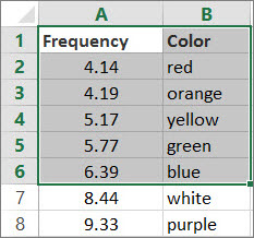
In the array form, LOOKUP evaluates the array and automatically changes behavior based on the array dimensions. If the array is wider than tall, LOOKUP looks for the lookup value in the first row of the array (like HLOOKUP). If the array is taller than wide (or square), LOOKUP looks for the lookup value in the first column (like VLOOKUP). In either case, LOOKUP returns a value at the same position from the last row or column in the array. The example below shows how the array form works. The formula in F5 is configured to use a vertical array and the formula in F6 is configured to use a horizontal array:
=LOOKUP(E5,B5:C9) // vertical array
=LOOKUP(E6,C11:G12) // horizontal array

The vertical and horizontal arrays contain the same values; only the orientation is different.
Note: Microsoft discourages the use of the array form and suggests VLOOKUP and HLOOKUP as better options.
Notes
- LOOKUP assumes that lookup_vector is sorted in ascending order.
- When lookup_value can’t be found, LOOKUP will match the next smallest value.
- When lookup_value is greater than all values in lookup_vector, LOOKUP matches the last value.
- When lookup_value is less than the first value in lookup_vector, LOOKUP returns #N/A.
- Result_vector must be the same size as lookup_vector.
- LOOKUP is not case-sensitive
This Excel tutorial explains how to use the Excel LOOKUP function with syntax and examples.
Description
The Microsoft Excel LOOKUP function returns a value from a range (one row or one column) or from an array.
The LOOKUP function is a built-in function in Excel that is categorized as a Lookup/Reference Function. It can be used as a worksheet function (WS) in Excel. As a worksheet function, the LOOKUP function can be entered as part of a formula in a cell of a worksheet.
There are 2 different syntaxes for the LOOKUP function:
LOOKUP Function (Syntax #1)
In Syntax #1, the LOOKUP function searches for value in the lookup_range and returns the value in the result_range that is in the same position.
The syntax for the LOOKUP function in Microsoft Excel is:
LOOKUP( value, lookup_range, [result_range] )
Parameters or Arguments
- value
- The value to search for in the lookup_range.
- lookup_range
- A single row or single column of data that is sorted in ascending order. The LOOKUP function searches for value in this range.
- result_range
- Optional. It is a single row or single column of data that is the same size as the lookup_range. The LOOKUP function searches for the value in the lookup_range and returns the value from the same position in the result_range. If this parameter is omitted, it will return the first column of data.
Returns
The LOOKUP function returns any datatype such as a string, numeric, date, etc.
If the LOOKUP function can not find an exact match, it chooses the largest value in the lookup_range that is less than or equal to the value.
If the value is smaller than all of the values in the lookup_range, then the LOOKUP function will return #N/A.
If the values in the LOOKUP_range are not sorted in ascending order, the LOOKUP function will return the incorrect value.
Example (as Worksheet Function)
Let’s look at some Excel LOOKUP function examples and explore how to use the LOOKUP function as a worksheet function in Microsoft Excel:
Based on the Excel spreadsheet above, the following LOOKUP examples would return:
=LOOKUP(10251, A1:A6, B1:B6)
Result: "Pears"

=LOOKUP(10251, A1:A6)
Result: 10251

=LOOKUP(10246, A1:A6, B1:B6)
Result: #N/A

=LOOKUP(10248, A1:A6, B1:B6)
Result: "Apples"
LOOKUP Function (Syntax #2)
In Syntax #2, the LOOKUP function searches for the value in the first row or column of the array and returns the corresponding value in the last row or column of the array.
The syntax for the LOOKUP function in Microsoft Excel is:
LOOKUP( value, array )
Parameters or Arguments
- value
- The value to search for in the array. The values must be in ascending order.
- array
- An array of values that contains both the values to search for and return.
Returns
The LOOKUP function returns any datatype such as a string, numeric, date, etc.
If the LOOKUP function can not find an exact match, it chooses the largest value in the lookup_range that is less than or equal to the value.
If the value is smaller than all of the values in the lookup_range, then the LOOKUP function will return #N/A.
If the values in the array are not sorted in ascending order, the LOOKUP function will return the incorrect value.
Example (as Worksheet Function)
Let’s look at some Excel LOOKUP function examples and explore how to use the LOOKUP function as a worksheet function in Microsoft Excel:
=LOOKUP("T", {"s","t","u","v";10,11,12,13})
Result: 11

=LOOKUP("Tech on the Net", {"s","t","u","v";10,11,12,13})
Result: 11

=LOOKUP("t", {"s","t","u","v";"a","b","c","d"})
Result: "b"

=LOOKUP("r", {"s","t","u","v";"a","b","c","d"})
Result: #N/A

=LOOKUP(2, {1,2,3,4;511,512,513,514})
Result: 512
Frequently Asked Questions
Question: In Microsoft Excel, I have a table of data in cells A2:D5. I’ve tried to create a simple LOOKUP to find CB2 in the data, but it always returns 0. What am I doing wrong?
Answer: Using the LOOKUP function can sometimes be a bit tricky so let’s look at an example. Below we have a spreadsheet with the data that you described.
In cell F1, we’ve placed the following formula:
=LOOKUP("CB2",A2:A5,D2:D5)
And yes, even though CB2 exists in the data, the LOOKUP function returns 0.
Now, let’s explain what is happening. At first, it looks like the function isn’t finding CB2 in the list, but in fact, it is finding something else. Let’s fill in the empty cells in D3:D5 to explain better.
If we place the values TEST1, TEST2, TEST3 in cells D3, D4, 5, respectively, we can see that the LOOKUP function is in fact returning the value TEST2. So we ask ourselves, when we are looking up CB2 in the data and CB2 exists in the data, why is it returning the value for CB19? Good question. The LOOKUP function assumes that the data in column A is sorted in ascending order.
If you look closer at column A, it is not in fact sorted in ascending order. If we quickly sorted column A, it would look like this:
Now the LOOKUP function correctly returns 3A when it is looking up CB2 in the data.
To avoid these sorting problems with your data, we recommend using VLOOKUP function in this case. Let’s show you how we would do this. If we changed our formula below (but left our data in column A in the original sort order):
The following VLOOKUP formula would return the correct value of 3A.
=VLOOKUP("CB2",$A$2:$D$5,4,FALSE)
The VLOOKUP function does not require us to have the data sorted in ascending order since we used FALSE as the last parameter — which means that it is looking for an exact match.
Question: I have the following LOOKUP formula:
=LOOKUP(C2,{"A","B","C","D","E","F","G","H","I","K","X","Z"}, {"1","2","3","4","5","6","7","8","9","10","12","1"})
I also need to add zero to the lookup vector and result vector. How do I do this?
Answer: Using numbers in Excel can be tricky, as you can enter them either as numeric or text values. Because of this, there are 2 possible solutions.
Numeric Solution
If you have entered your zero as a numeric value, then the following formula will work:
=LOOKUP(C2,{0,"A","B","C","D","E","F","G","H","I","K","X","Z"}, {0,"1","2","3","4","5","6","7","8","9","10","12","1"})
Text Solution
If you have entered your zero as a text value, then the following formula will work:
=LOOKUP(C2,{"0","A","B","C","D","E","F","G","H","I","K","X","Z"}, {"0","1","2","3","4","5","6","7","8","9","10","12","1"})
Question: For the following function in Microsoft Excel:
=LOOKUP(M14,Sheet2!A2:A2240,Sheet2!B2:B2240)
How do I get it to return a blank cell if the LOOKUP value (M14) is blank?
Answer: To check for a blank value in cell M14, you can use the IF function and ISBLANK function as follows:
=IF(ISBLANK(M14),"",LOOKUP(M14,Sheet2!A2:A2240,Sheet2!B2:B2240))
Now if the value in cell M14 is blank, the formula will return a blank. Otherwise it will perform the LOOKUP function as before.