
Содержание
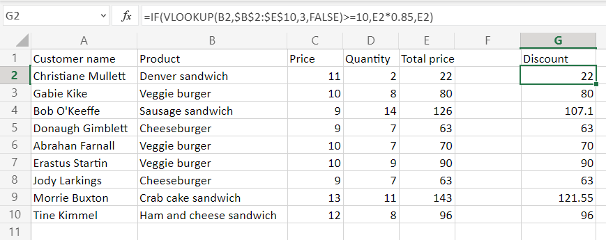
- LOOKUP function
- There are two ways to use LOOKUP: Vector form and Array form
- Vector form
- Syntax
- Remarks
- Vector examples
- Array form
- Syntax
- XLOOKUP With If Statement – Excel & Google Sheets
- XLOOKUP Multiple Lookup Criteria
- Logical Criteria
- Array AND
- XLOOKUP Function
- XLOOKUP Error-Handling with IF
- XLOOKUP IF with ISNA
- ISNA Function
- IF Function
- XLOOKUP IF with ISBLANK
- ISBLANK Function
- IF Function
- XLOOKUP IF with ISTEXT
- ISTEXT Function
- IF Function
- XLOOKUP with IFS
- ISNA
- ISBLANK and ISTEXT
- Default Value
LOOKUP function
Use LOOKUP, one of the lookup and reference functions, when you need to look in a single row or column and find a value from the same position in a second row or column.
For example, let’s say you know the part number for an auto part, but you don’t know the price. You can use the LOOKUP function to return the price in cell H2 when you enter the auto part number in cell H1.
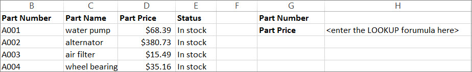
Use the LOOKUP function to search one row or one column. In the above example, we’re searching prices in column D.
Tips: Consider one of the newer lookup functions, depending on which version you are using.
Use VLOOKUP to search one row or column, or to search multiple rows and columns (like a table). It’s a much improved version of LOOKUP. Watch this video about how to use VLOOKUP.
If you are using Microsoft 365, use XLOOKUP — it’s not only faster, it also lets you search in any direction (up, down, left, right).
There are two ways to use LOOKUP: Vector form and Array form
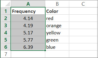
Vector form: Use this form of LOOKUP to search one row or one column for a value. Use the vector form when you want to specify the range that contains the values that you want to match. For example, if you want to search for a value in column A, down to row 6.
Array form: We strongly recommend using VLOOKUP or HLOOKUP instead of the array form. Watch this video about using VLOOKUP. The array form is provided for compatibility with other spreadsheet programs, but it’s functionality is limited.
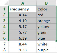
An array is a collection of values in rows and columns (like a table) that you want to search. For example, if you want to search columns A and B, down to row 6. LOOKUP will return the nearest match. To use the array form, your data must be sorted.
Vector form
The vector form of LOOKUP looks in a one-row or one-column range (known as a vector) for a value and returns a value from the same position in a second one-row or one-column range.
Syntax
LOOKUP(lookup_value, lookup_vector, [result_vector])
The LOOKUP function vector form syntax has the following arguments:
lookup_value Required. A value that LOOKUP searches for in the first vector. Lookup_value can be a number, text, a logical value, or a name or reference that refers to a value.
lookup_vector Required. A range that contains only one row or one column. The values in lookup_vector can be text, numbers, or logical values.
Important: The values in lookup_vector must be placed in ascending order: . -2, -1, 0, 1, 2, . A-Z, FALSE, TRUE; otherwise, LOOKUP might not return the correct value. Uppercase and lowercase text are equivalent.
result_vector Optional. A range that contains only one row or column. The result_vector argument must be the same size as lookup_vector. It has to be the same size.
If the LOOKUP function can’t find the lookup_value, the function matches the largest value in lookup_vector that is less than or equal to lookup_value.
If lookup_value is smaller than the smallest value in lookup_vector, LOOKUP returns the #N/A error value.
Vector examples
You can try out these examples in your own Excel worksheet to learn how the LOOKUP function works. In the first example, you’re going to end up with a spreadsheet that looks similar to this one:
Copy the data in following table, and paste it into a new Excel worksheet.
Copy this data into column A
Copy this data into column B
Next, copy the LOOKUP formulas from the following table into column D of your worksheet.
Copy this formula into the D column
Here’s what this formula does
Here’s the result you’ll see
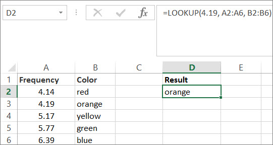
=LOOKUP(4.19, A2:A6, B2:B6)
Looks up 4.19 in column A, and returns the value from column B that is in the same row.
=LOOKUP(5.75, A2:A6, B2:B6)
Looks up 5.75 in column A, matches the nearest smaller value (5.17), and returns the value from column B that is in the same row.
=LOOKUP(7.66, A2:A6, B2:B6)
Looks up 7.66 in column A, matches the nearest smaller value (6.39), and returns the value from column B that is in the same row.
=LOOKUP(0, A2:A6, B2:B6)
Looks up 0 in column A, and returns an error because 0 is less than the smallest value (4.14) in column A.
For these formulas to show results, you may need to select them in your Excel worksheet, press F2, and then press Enter. If you need to, adjust the column widths to see all the data.
Array form
Tip: We strongly recommend using VLOOKUP or HLOOKUP instead of the array form. See this video about VLOOKUP; it provides examples. The array form of LOOKUP is provided for compatibility with other spreadsheet programs, but its functionality is limited.
The array form of LOOKUP looks in the first row or column of an array for the specified value and returns a value from the same position in the last row or column of the array. Use this form of LOOKUP when the values that you want to match are in the first row or column of the array.
Syntax
The LOOKUP function array form syntax has these arguments:
lookup_value Required. A value that LOOKUP searches for in an array. The lookup_value argument can be a number, text, a logical value, or a name or reference that refers to a value.
If LOOKUP can’t find the value of lookup_value, it uses the largest value in the array that is less than or equal to lookup_value.
If the value of lookup_value is smaller than the smallest value in the first row or column (depending on the array dimensions), LOOKUP returns the #N/A error value.
array Required. A range of cells that contains text, numbers, or logical values that you want to compare with lookup_value.
The array form of LOOKUP is very similar to the HLOOKUP and VLOOKUP functions. The difference is that HLOOKUP searches for the value of lookup_value in the first row, VLOOKUP searches in the first column, and LOOKUP searches according to the dimensions of array.
If array covers an area that is wider than it is tall (more columns than rows), LOOKUP searches for the value of lookup_value in the first row.
If an array is square or is taller than it is wide (more rows than columns), LOOKUP searches in the first column.
With the HLOOKUP and VLOOKUP functions, you can index down or across, but LOOKUP always selects the last value in the row or column.
Important: The values in array must be placed in ascending order: . -2, -1, 0, 1, 2, . A-Z, FALSE, TRUE; otherwise, LOOKUP might not return the correct value. Uppercase and lowercase text are equivalent.
Источник
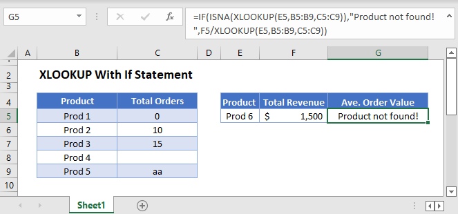
XLOOKUP With If Statement – Excel & Google Sheets
This tutorial will demonstrate how to combine the XLOOKUP and IF functions in Excel. If your version of Excel does not support XLOOKUP, read how to use VLOOKUP instead.
XLOOKUP Multiple Lookup Criteria
There are a lot of ways to use the IF Function alongside the XLOOKUP Function, but first, let’s look at an example using the core element of the IF Function, the logical criteria.
One common example is performing a lookup with multiple criteria, and the most common solution to this is by concatenating the lookup criteria (e.g., F3&G3) and their corresponding column in the lookup data (e.g., B3:B7&C3:C7).
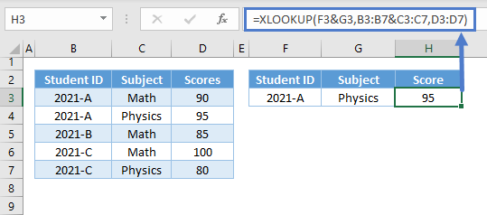
The above method works fine most of the time, but it can lead to incorrect results for conditions that involve numbers.
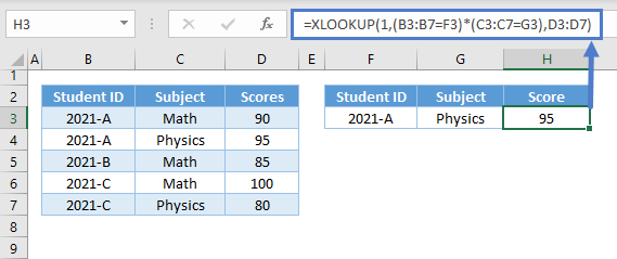
A more foolproof method is by creating an array of Boolean values from logical criteria.
Let’s walk through this formula:
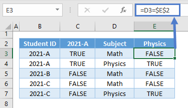
Logical Criteria
First, let’s apply the appropriate condition to their corresponding columns by using the logical operators (e.g., =, ).
Let’s start with the first criterion (e.g., Student ID).
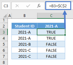
Repeat the step for the other criteria (e.g., Subject).
Array AND
Next, we perform the array equivalent of the AND Function by multiplying the Boolean arrays where TRUE is 1 and FALSE is 0.
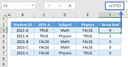
Note: The AND Function is an aggregate function (many inputs to one output). Therefore, it won’t work in our array scenario.
XLOOKUP Function
Next, we use the result of the Array AND as the new lookup array where we will lookup for 1 instead of the original lookup value.
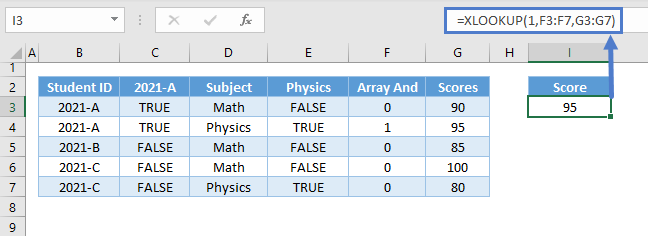
Combining all formulas above results to our original formula:
XLOOKUP Error-Handling with IF
Sometimes we need to check if the result of an XLOOKUP Function results in an error. A great way of doing this is by using the IF Function, which is also the best way of notifying us about the cause of the error.
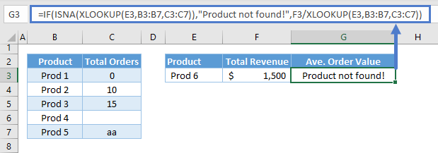
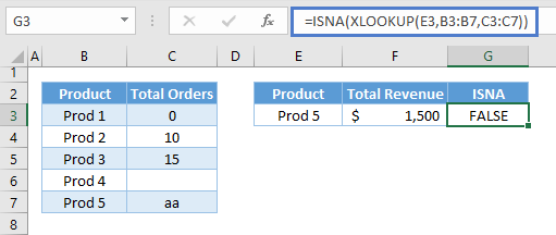
XLOOKUP IF with ISNA
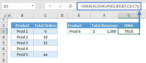
Let’s first check if the XLOOKUP failed to find a match using the IF with ISNA Formula.
Let’s walk through the above formula:
ISNA Function
First, let’s check for the #N/A Error, which basically means no match was found, using the ISNA Function.
IF Function
Next, let’s use the IF Function to check the result of the ISNA Function and return a message (e.g., “Product not found!”) if the result is TRUE. Otherwise, if the result is false, we’ll proceed with the calculation.
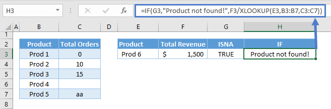
Combining all formulas results to our original formula:
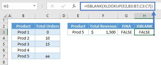
XLOOKUP IF with ISBLANK
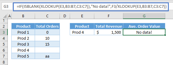
Another thing to check is if the result of XLOOKUP is blank. There are cases where blank means there’s no input yet, and therefore, we need to distinguish it from zero.
We’ll just replace the ISNA with ISBLANK to check for blank.
Let’s walk through the above formula:
ISBLANK Function
First, let’s check for blank using the ISBLANK Function.

IF Function
Just like with the previous scenario, we then input the result of the ISBLANK Function to the IF Function and return a message (e.g., “No Data!”) if TRUE or proceed with the calculation if FALSE.
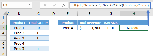
Combining all formulas results to our original formula:

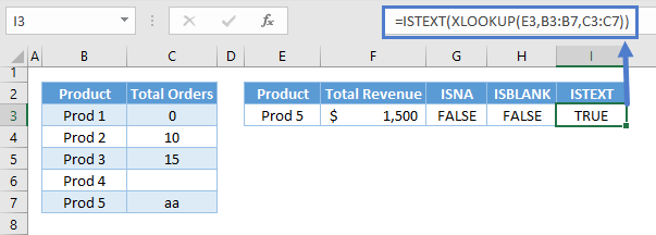
XLOOKUP IF with ISTEXT
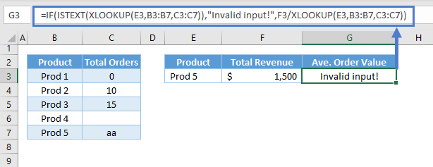
Another thing to avoid in calculations is accidental text input. In this case, we’ll use the IF with ISTEXT Formula to check for a text value.
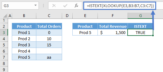
ISTEXT Function
First, we check if the output of the XLOOKUP Function is a text.
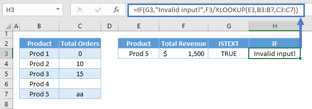
IF Function
Next, we check the result using the IF Function and return the corresponding message (e.g., “Invalid input!”) if TRUE or proceed to the calculation if FALSE.
XLOOKUP with IFS
The final error-handling formula would be the combination of the previous IF Formulas, and we can do this by nesting them.
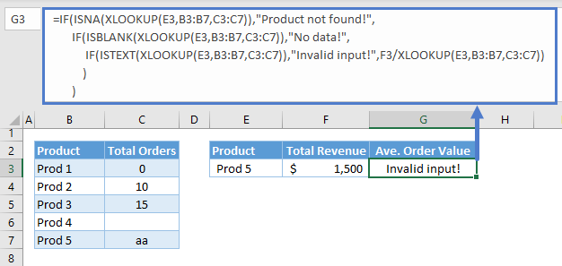
As we notice above, the Nested IF Formula becomes more complicated as we add more conditions. A better way to approach this is by using the IFS Function.
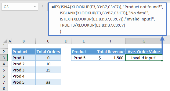
Note: The IFS Function can evaluate multiple sets of logical criteria. It starts from the first condition moving on to the next until it finds the first TRUE condition and returns the corresponding return value to it.
Let’s walk through the formula above:
ISNA
We start with our first condition, which is the ISNA Function. If ISNA is TRUE, we return its corresponding value (e.g., “Product not found!”). Otherwise, we proceed to check the next condition.
ISBLANK and ISTEXT
Since the first condition is FALSE in this scenario, we check the succeeding conditions until we find the first TRUE and return the corresponding value for the TRUE condition.
Default Value
We can set a default value by setting the last condition as TRUE in case all the conditions are FALSE, which in our error-handling scenario, means that we can now proceed to the calculation without errors.
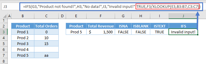
Combining all formulas above results to our original formula:
Источник
VLOOKUP in Excel is a function to make vertical lookups. IF is the Excel function to run logical comparisons (TRUE or FALSE). Separately, they can do a great job. However, you can nest Excel VLOOKUP and IF, and enjoy their synergy. Read on to discover their uses.
How to use IF and VLOOKUP in Excel together
In most cases, you can use the Excel VLOOKUP IF statements to make a comparison between a lookup result and a specified value. At the same time, IF VLOOKUP Excel can also cope with the following tasks:
- Do a vertical lookup on two values
- Conceal #N/A errors
- Perform calculations
Check out how to use VLOOKUP in Excel
=IF(VLOOKUP("lookup_value",lookup_range, column_number, [match])logical_condition, value_if_true, value_if_false)"lookup_value"– the value to look up vertically.lookup_range– the range of where to search for the lookup_value and the matching value.column_number– the number of the column containing the matching value to return.[match]is an optional parameter to choose either closest match (TRUE) or exact match (FALSE). TRUE is set by default.logical_condition– a logical expression that can be evaluated as TRUE or FALSE. Logical expressions are built with the help of logical operators: =, >, =<, etc.value_if_true– the value to return if thelogical_conditionis TRUE.value_if_false– the value to return if thelogical_conditionis FALSE.
VLOOKUP with IF condition in Excel example
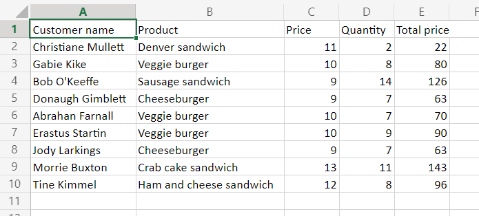
To demonstrate how the Excel IF function with VLOOKUP works, we imported a data set from Airtable to Excel using Coupler.io, a tool for integrating different sources such as Airtable, Google Sheets, or BigQuery with Excel.
Check out the available Excel integrations and try out Coupler.io for your project.
Our goal consists of two steps, implemented in one IF VLOOKUP formula in Excel:
- Find a quantity that matches the lookup value
"Sausage sandwich" - Get a notification “Bon Appetit!” if the return value is greater than 10. If not, get a notification “Not bad“.
Here is what the formula looks like:
=IF(VLOOKUP(B4,B3:E12,3,FALSE)>10, "Bon Appetit!", "Not bad")
Now let’s check out other ways of using Excel IF and VLOOKUP together.
Excel IF statement with VLOOKUP to do a vertical lookup on two values
The idea here is slightly different from the example above. You have a logical condition based on which you can perform two vertical lookups:
- Do the first lookup if the condition is true.
- Do the second lookup if the condition is false.
For example, if we have “Erastus Startin” in cell G2, then the formula will perform VLOOKUP on the type of sandwich that matches this value; otherwise, it will perform VLOOKUP on the Tine Kimmel’s type of sandwich. Here is what the IF VLOOKUP Excel formula looks like:
=IF(G2="Erastus Startin", VLOOKUP("Erastus Startin",A1:E10,2,FALSE), VLOOKUP("Tine Kimmel",A1:E10,2,FALSE))

This example may look illogical, but it explains the mechanism of using IF and VLOOKUP for two values.
Check out our blog post about Excel VLOOKUP between two values.
Now let’s see how you can use the combination of these functions to hide #N/A errors.
Excel formulas VLOOKUP IF to conceal #N/A errors
We have a lookup list and we need to learn which of the values from the dataset are on this list.

We can use a regular combination of IF and VLOOKUP like this:
=IF(B2=VLOOKUP(B2,$H$2:$H$4,1,FALSE),"Yes","No")

However, if we drag the formula down, we’ll get #N/A errors instead of the expected “No“.

This can be fixed if we slightly update our formula by adding the ISNA function as follows:
=IF(ISNA(VLOOKUP(B2,$H$2:$H$4,1,FALSE)),"No","Yes")

IFNA instead of Excel IF ISNA VLOOKUP to conceal #N/A errors
The Excel IFNA function is another option to use for hiding #N/A errors in the IF VLOOKUP formulas. However, the drawback of this function is that you can only specify the value to return instead of #N/A errors. Here is how it looks in our example:
=IFNA(VLOOKUP(B2,$H$2:$H$4,1,FALSE),"No")

Excel IF and VLOOKUP for calculations
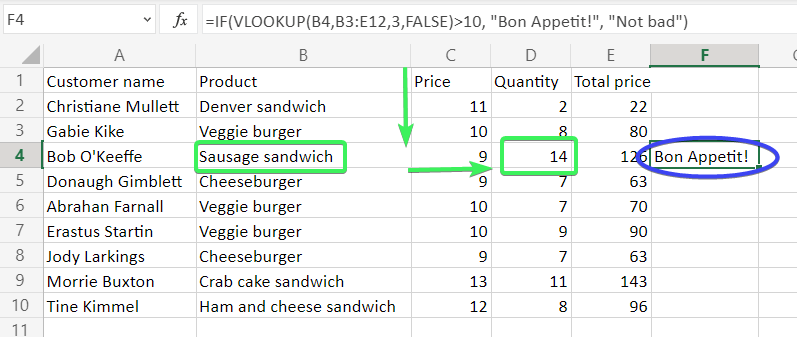
You can expand your IF VLOOKUP formula with arithmetic operators to perform calculations based on a specified condition. In our example, we want to vlookup the orders with 10+ items and provide them with a 15% discount. Here is the formula to make this happen:
=IF(VLOOKUP(B2,$B$2:$E$10,3,FALSE)>=10,E2*0.85,E2)
VLOOKUP(B2,$B$2:$E$10,3,FALSE)>=10– condition for a vlookup resultE2*0.85– the total amount including the 15% discount if the condition is true
IF VLOOKUP Excel is powerful pairing
These two Excel functions nested together can solve many problems. At the same time, separately they can also do many things, for example, compare two columns in Excel using VLOOKUP or run different logical checks using IF. Additionally, you can use these functions nested with others, such as SUM, SUMIF, COUNTIF, and many more. Good luck with your data!
-

A content manager at Coupler.io whose key responsibility is to ensure that the readers love our content on the blog. With 5 years of experience as a wordsmith in SaaS, I know how to make texts resonate with readers’ queries✍🏼

Back to Blog
Focus on your business
goals while we take care of your data!
Try Coupler.io
VLOOKUP is a powerful function to perform lookup in Excel. It performs a row-wise lookup until a match is found. The IF function performs a logical test and returns one value for a TRUE result, and another for a FALSE result. IF and VLOOKUP functions are used together in multiple cases: to compare VLOOKUP results, to handle errors, to lookup based on two values. To use the IF and VLOOKUP functions together you should nest the VLOOKUP function inside the IF function.
Combine IF Function with VLOOKUP
You can use IF and VLOOKUP together nesting the VLOOKUP function inside the IF function. The following will present a more detailed overview of the uses of IF function with VLOOKUP.
Comparing values to VLOOKUP result
IF and VLOOKUP are used together mostly to compare the results of VLOOKUP to another value. In the following example, based on the list in cells A1:B6, to find out if the name mentioned in cell D2 has a bonus which is based on sales over $2,500:
- Select cell E2 by clicking on it.
- Assign the formula
=IF(VLOOKUP(D2,A2:B6,2,FALSE)>2500,"Yes","No")to cell E2. - Press Enter to apply the formula in cell E2.
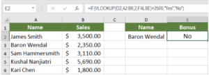
This will return the result No as Baron Wendal had sales of $2,350. You can also compare VLOOKUP results to cell values in a similar way. All you need to do is to set the cell reference as the condition inside the IF function.
Handling errors
Another common use of IF function with VLOOKUP is to handle errors. In the previous example, assign the value Jason Williams to cell D2. To find the sales, assign the formula = VLOOKUP(D2,A2:B6,2,FALSE) to cell E2.
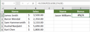
This will return a #N/A error. The name Jason Williams does not exist in cells A2:A6. To handle this error with your own custom message, you will nest the VLOOKUP and ISNA functions inside an IF function. To do that:
- Select cell E2 by clicking on it.
- Assign the formula =
IF(ISNA(VLOOKUP(D2,A2:B6,2,FALSE)),"Name not found",VLOOKUP(D2,A2:B6,2,FALSE))to cell E2. - Press enter to apply the formula to cell E2.
This will return Name not found. The ISNA function checks if the result of the VLOOKUP is a #N/A error, and executes the corresponding IF condition. You can set other text messages or even a 0 or blank (“”) as the output.
Lookup Based on two values
You can also use IF and VLOOKUP together to perform a lookup based on two values. In this example, cells A1:C6 contains the price for products in two different shops. To find the price of the product in cell E2:
- Select cell G2 by clicking on it.
- Assign the formula
=IF(F2="Shop 1",VLOOKUP(E2,A2:C6,2,FALSE),VLOOKUP(E2,A2:C6,3,FALSE))to cell G2. - Apply the formula to G2 by pressing Enter.
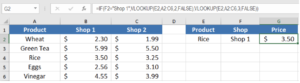
This will return $3.50. The IF function checks if the value in cell F2 is Shop 1 or 2. According to this condition, the VLOOKUP then returns the corresponding price for the product.
Excel has several very effective functions when it comes to lookup values in other columns. One of these functions is VLOOKUP. It is a very powerful lookup and reference function for looking up data. Combined with the IF function, VLOOKUP can perform more advanced lookups that help to analyze data more effectively.
Still need some help with Excel formatting or have other questions about Excel? Connect with a live Excel expert here for some 1 on 1 help. Your first session is always free.
Are you still looking for help with the IF function? View our comprehensive round-up of IF function tutorials here.
See Also:
How to Use a VLOOKUP in Excel – Excelchat
How to Use a VLOOKUP in Google Sheets – Excelchat
VLOOKUP Not Working? (Find Out Why) – Excelchat
How to Use VLOOKUP with Multiple Criteria – Excelchat
INDEX MATCH versus VLOOKUP: How and When to Use – Excelchat
How to Use VLOOKUP across Multiple Sheets in Excel – Excelchat
How to Use VLOOKUP with Multiple Workbooks – Excelchat
Use LOOKUP, one of the lookup and reference functions, when you need to look in a single row or column and find a value from the same position in a second row or column.
For example, let’s say you know the part number for an auto part, but you don’t know the price. You can use the LOOKUP function to return the price in cell H2 when you enter the auto part number in cell H1.
Use the LOOKUP function to search one row or one column. In the above example, we’re searching prices in column D.
Tips: Consider one of the newer lookup functions, depending on which version you are using.
-
Use VLOOKUP to search one row or column, or to search multiple rows and columns (like a table). It’s a much improved version of LOOKUP. Watch this video about how to use VLOOKUP.
-
If you are using Microsoft 365, use XLOOKUP — it’s not only faster, it also lets you search in any direction (up, down, left, right).
There are two ways to use LOOKUP: Vector form and Array form
-
Vector form: Use this form of LOOKUP to search one row or one column for a value. Use the vector form when you want to specify the range that contains the values that you want to match. For example, if you want to search for a value in column A, down to row 6.

-
Array form: We strongly recommend using VLOOKUP or HLOOKUP instead of the array form. Watch this video about using VLOOKUP. The array form is provided for compatibility with other spreadsheet programs, but it’s functionality is limited.
An array is a collection of values in rows and columns (like a table) that you want to search. For example, if you want to search columns A and B, down to row 6. LOOKUP will return the nearest match. To use the array form, your data must be sorted.
Vector form
The vector form of LOOKUP looks in a one-row or one-column range (known as a vector) for a value and returns a value from the same position in a second one-row or one-column range.
Syntax
LOOKUP(lookup_value, lookup_vector, [result_vector])
The LOOKUP function vector form syntax has the following arguments:
-
lookup_value Required. A value that LOOKUP searches for in the first vector. Lookup_value can be a number, text, a logical value, or a name or reference that refers to a value.
-
lookup_vector Required. A range that contains only one row or one column. The values in lookup_vector can be text, numbers, or logical values.
Important: The values in lookup_vector must be placed in ascending order: …, -2, -1, 0, 1, 2, …, A-Z, FALSE, TRUE; otherwise, LOOKUP might not return the correct value. Uppercase and lowercase text are equivalent.
-
result_vector Optional. A range that contains only one row or column. The result_vector argument must be the same size as lookup_vector. It has to be the same size.
Remarks
-
If the LOOKUP function can’t find the lookup_value, the function matches the largest value in lookup_vector that is less than or equal to lookup_value.
-
If lookup_value is smaller than the smallest value in lookup_vector, LOOKUP returns the #N/A error value.
Vector examples
You can try out these examples in your own Excel worksheet to learn how the LOOKUP function works. In the first example, you’re going to end up with a spreadsheet that looks similar to this one:
-
Copy the data in following table, and paste it into a new Excel worksheet.
Copy this data into column A
Copy this data into column B
Frequency
4.14
Color
red
4.19
orange
5.17
yellow
5.77
green
6.39
blue
-
Next, copy the LOOKUP formulas from the following table into column D of your worksheet.
Copy this formula into the D column
Here’s what this formula does
Here’s the result you’ll see
Formula
=LOOKUP(4.19, A2:A6, B2:B6)
Looks up 4.19 in column A, and returns the value from column B that is in the same row.
orange
=LOOKUP(5.75, A2:A6, B2:B6)
Looks up 5.75 in column A, matches the nearest smaller value (5.17), and returns the value from column B that is in the same row.
yellow
=LOOKUP(7.66, A2:A6, B2:B6)
Looks up 7.66 in column A, matches the nearest smaller value (6.39), and returns the value from column B that is in the same row.
blue
=LOOKUP(0, A2:A6, B2:B6)
Looks up 0 in column A, and returns an error because 0 is less than the smallest value (4.14) in column A.
#N/A
-
For these formulas to show results, you may need to select them in your Excel worksheet, press F2, and then press Enter. If you need to, adjust the column widths to see all the data.
Array form
The array form of LOOKUP looks in the first row or column of an array for the specified value and returns a value from the same position in the last row or column of the array. Use this form of LOOKUP when the values that you want to match are in the first row or column of the array.
Syntax
LOOKUP(lookup_value, array)
The LOOKUP function array form syntax has these arguments:
-
lookup_value Required. A value that LOOKUP searches for in an array. The lookup_value argument can be a number, text, a logical value, or a name or reference that refers to a value.
-
If LOOKUP can’t find the value of lookup_value, it uses the largest value in the array that is less than or equal to lookup_value.
-
If the value of lookup_value is smaller than the smallest value in the first row or column (depending on the array dimensions), LOOKUP returns the #N/A error value.
-
-
array Required. A range of cells that contains text, numbers, or logical values that you want to compare with lookup_value.
The array form of LOOKUP is very similar to the HLOOKUP and VLOOKUP functions. The difference is that HLOOKUP searches for the value of lookup_value in the first row, VLOOKUP searches in the first column, and LOOKUP searches according to the dimensions of array.
-
If array covers an area that is wider than it is tall (more columns than rows), LOOKUP searches for the value of lookup_value in the first row.
-
If an array is square or is taller than it is wide (more rows than columns), LOOKUP searches in the first column.
-
With the HLOOKUP and VLOOKUP functions, you can index down or across, but LOOKUP always selects the last value in the row or column.
Important: The values in array must be placed in ascending order: …, -2, -1, 0, 1, 2, …, A-Z, FALSE, TRUE; otherwise, LOOKUP might not return the correct value. Uppercase and lowercase text are equivalent.
-
In this article, we will learn how to use Excel ISNA function with VLOOKUP to ignore the #N/A error while calculating the formula in MS Excel 2016.
Excel VLOOKUP function is used to look up and fetch data from a specific column of a table. The «V» stands for «vertical». Lookup values must appear in the first column of the table, with lookup columns to the right.
How to use the Vlookup function in excel?
VLOOKUP function in Excel is used to look up and retrieve data from a specific column of a table.
Syntax:
=VLOOKUP(lookup_value, table_array, col_index_num, [range_lookup])
How to use the ISNA function in excel?
ISNA function used for checking the #N/A error while calculation by using any function.
Syntax:
How to use the if function in excel?
IF function works on logic_test and returns values based on the result of the test.
Syntax:
=IF(Logic_test, [Value_if_True], [Value_if_False])
Let’s get this with an example.
Here we have two sheets, we have to get the BIRTHDT from SHEET 1 table to SHEET 2 Table using the functions.
SHEET 1:
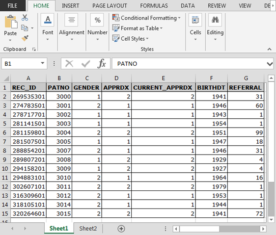
SHEET 2:

Write the formula in C2 cell of SHEET 2.
Explanation:
Vlookup function in excel looks for the 6th column of the SHEET 1 matching REC_ID in SHEET 1 from SHEET 2.
ISNA function in excel looks for the #NA error and passes it on to IF function.
IF formula in excel checks if any #NA error occurs, it print “NotFound” instead of the #NA error.
Copy the formula in other cells, select the cells including the first cell where the formula is already applied, use shortcut key Ctrl + D.
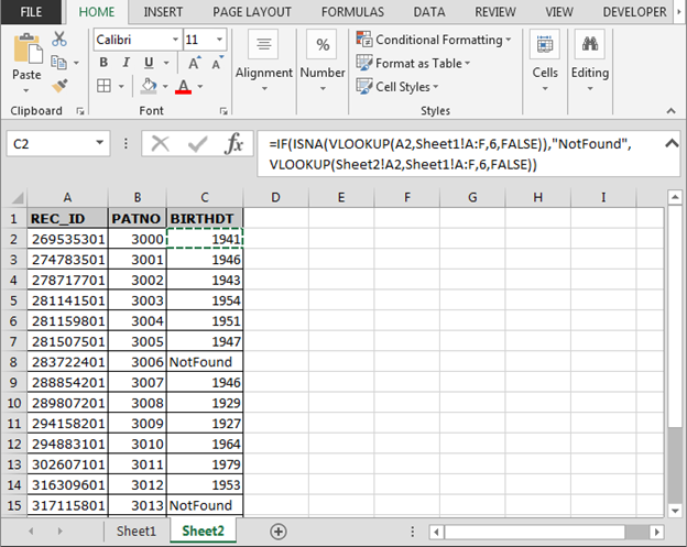
As you can see in the above image, the formula is working fine. And the user can work without getting irritated by #NA error.
Hope you understood IF, ISNA and VLOOKUP function in Excel 2016, 2013 and 2010. There are more articles on VLOOKUP Examples and HLOOKUP Examples here. Please do check more links here and if you have any unresolved query, please state that in the comment box below. We will help you.
Below are the examples to learn more:-
Two-way table lookups — can’t get the function to work
Question asked by user:-
If anybody can help with this I’m trying to get the correct price from the table from the data entered in AB2 and AB3. The function used is in cell AB7.
Click here:- How to use ISNA function along with INDEX and MATCH function?
IF Statement combining multiple ‘IF TRUE’ conditions
Question asked by user:-
Assuming that I have a worksheet with columns A,B,C and D on it, now I want an IF statement in column E which follows this argument:
IF A1 is «0» or «N/A», then show N/A, but if A1 is any other number, then B*(C+D)
I hope that’s easy to follow. I have tried so hard to get this to work but just can’t.
As ever, any help would be hugely appreciated.
Click here:- How to use ISNA with nested IF condition?
Related Articles:
ISERROR and VLOOKUP function
IFERROR and VLOOKUP function
VLOOKUP Multiple Values
Partial match with VLOOKUP function
In This Chapter
Using IF to take a course of action
Returning a value with CHOOSE
Applying logic
Finding where values are Looking up values in a table Transposing data
Decisions, decisions! If one of our students gets an 88 on the test, is that a #*^B+ or is it an A? If our company’s new product earns at least $15,000 in revenue, how much bonus should we give out to the team? Or do we have to get to $20,000 before we do that? How does this affect the financial statements?
Excel cannot make decisions for you but it can help you make better decisions. Using functions, such as IF and CHOOSE, you can set up your worksheet to chart a course through the possibilities. Hey, things could be worse! Were it not for Excel, you might have to try the old Ouija board technique.
Have a busy worksheet? Data all over the place? It’s okay to admit it. That’s what we’re here for! In this chapter, we are going to show you a slew of functions that make it easy to look up information that’s spread around the rows and columns.
Speaking of data, did you ever mistakenly organize your information along a row or rows and then realize that you are going to run out of room! Yes, us too. Been there, done that. What started out as a project to track some stocks became a problem when the number of stocks grew past 256. In case you are not aware, there are only 256 columns available in Excel! The project got so big we were going to run out of room. Help!
The answer was of course to reorient the information to go down a column. Whew, lucky us! Excel provides the TRANSPOSE function to take care of this!
It’s a good thing an Excel worksheet has 65,536 columns. That gives plenty of wiggle room!
By the way this was paper trading, otherwise there would not have been 256 stocks in the portfolio. Did pretty well though!
Testing on One Condition
The IF function is like the Swiss Army knife of Excel functions. Really, it is used in many situations. Often it is used with other functions. You see quite a bit of that in this chapter.
IF, structurally, is easy to understand. The function takes three arguments, but with a caveat. The second argument or the third argument is used, but never both. The three arguments are:
1. A test that gives a true or false answer.
For example, the test “is A5=A8″ is either true or false. We are not looking for a result of a calculation here. Adding A5 with A8 (A5 + A8) would produce an error.
2. What to do if the test if true.
3. What to do if the test is false.
Sounds easy enough. Here are some examples:
| Function | Comment | |
| =IF(D10>D20, | D10, D20) | If the value in D10 is greater than the value in D20 then the value in D10 is returned because the test is true. If the value in D10 is not greater than D20 than the value in D20 is returned. If the values in D10 and D20 are equal, the test returns false and the value in D20 is returned. |
| =IF(D10>D20, “Good news!”, “Bad news!”) | If the value in D10 is greater than the value in D20, then “Good News!” is returned. Otherwise “Bad News!” is returned. | |
| =IF(D10>D20, “Bad news!”) | “”, | If the value in D10 is greater than the value in D20, then nothing is returned. Otherwise “Bad News!” is returned. Note that the second argument is empty. |
| =IF(D10>D20, “Good news!”, | “”) | If the value in D10 is greater than the value in D20, then “Good News!” is returned. Otherwise nothing is returned. Not that the third argument is empty. |
An important aspect to note about using IF is the option of letting the second or third argument return nothing. Actually what is returned is an empty string, and the best way to do this is to place two double quote marks together with nothing in the middle.
IF therefore lets you set up two specific actions to take — one for when the test is true and another for when the test is false. Or, you can specify one test to take for either the true or false result, and do nothing for the opposite result.
As seen in the previous example, a common use of IF is to see how two values compare to each other, and return either one value or the other, depending of course on how you set up the test in the first argument.
IF is often used as a validation check to avoid errors. The probable best use of this is to avoid a division by 0 error. Simply put, wherever you have a division operation in you worksheet, you can instead use an IF to avoid an error if the denominator is 0. For example, this formula:
![]()
is replaced with this one:
![]()
Think of what would happen if G4 was ever 0. You would get the dreaded #DIV/0! error! But this can never happen if you put the division operation in the IF statement. If G4 is ever 0, then 0 is the result. The test is to see if G4 is not equal to 0. If G4 is not equal to 0 then the division operation occurs because the test is true. If G4 is 0, then the third argument (the action to take when the test is false) says to instead just return 0. You can write the function to take a different action, such as to return a statement such as Cannot complete calculation.
Note too that in this example, the true action is taken even if G4 is less than 0. That’s mathematically okay, but may not be what you need. Perhaps you need to make sure G4 is greater than 0, such as this:
![]()
One of the all time favorite uses of the IF function is to test for 0 in the denominator of a division operation. Then an action can be taken to avoid a division by 0 error.
Figure 14-1 shows how IF can be put to good use in a business application. A fictitious guitar shop — ” Guitars” (kinda snappy, don’t you think!) — keeps tabs on inventory in an Excel worksheet.

Figure 14-1:
Keeping an eye on inventory at the guitar shop.
Column D shows the inventory levels, and column E shows the reorder levels. The way this works is when a products’ inventory level is the same or less than the reorder level than it is time to order more of the product. (We don’t know about you but we love the thought of being surrounded by a bunch of stratoblasters!)
The cells in column F contain a formula. Here is the formula in cell F8:
![]()
What this says is that if the number of Stratoblaster 9000 guitars in stock is the same or less than the reorder level, then return Order. If the number in stock is greater than the reorder level, then nothing is returned. There are three in stock and the reorder level is two, therefore nothing is returned.
In the next row, the number of Flying X’s is equal to the reorder level, therefore cell F9 displays Order.
Using IF is easy. Just remember there are three arguments: The test, the action to take when the test is true, and the action to take when the test is false. Try it out:
1. Enter two values in a worksheet.
These values should have some meaning to you, such as the inventory levels example in Figure 14-1.
2. Click the cell where you want the result to appear.
3. Enter =IF( to start the function.
4. Decide on what test you want to perform.
You can test to see if the two values equal each other; if one is larger than the other; if subtracting one from the other is greater than, equal to, or less than 0; and so on. For example, to test if the first value equals the second value, click the first cell (or enter its address), enter an equal sign (=), and then finally click the second cell (or enter its address).
5. Enter a comma (,).
6. Enter the result that should appear if the test is true.
For example, enter The values are equal.
7. Enter a comma (,).
8. Enter the result that should appear if the test is false.
For example, enter The values are not equal.
9. Enter a closing parenthesis to end the function and press Enter.
The IF function can do a whole lot more, as you see next. Nested IF functions offer a bunch of possibilities on what value to return. A bit of perseverance is necessary to get through this.
You can place an IF function inside another IF function. That is, the inner IF is placed where the true or false argument in the outer IF goes (or even use internal IFs for both of the arguments). Why would you do this?
The other night we were deciding where to go out for dinner. Our thought was if the restaurant is Italian, then if they serve manicotti, then we will have manicotti, otherwise we will just eat pizza.
Logically this decision looks like this:

This looks a lot like programming code. we have left out the End If statements on purpose to avoid confusion because the IF function has no equivalent value.
That’s it! Make note that the inner IF statement has a result for both the true and false possibilities. The outer IF does not. Here is the structure of this as nested Excel IF statements:
=IF(Restaurant=Italian, IF(Restaurant serves manicotti, “manicotti”, “pizza”), “”)
Wow, if the restaurant was not Italian, then it didn’t matter what we ate. Literally this is true according to how this is structured. The third argument of the outer IF is empty.
You can nest up to seven IF statements.
Apply a nested IF statement to the inventory worksheet from Figure 14-1. Figure 14-2 has an additional column — Hot Item. A Hot Item takes two forms:
If the inventory level is half or less of the reorder level, and the last order date is within the last 30 days, then this is a Hot Item. The point of view is that in 30 days or less the stock sold down to half or less than the reorder level. This means the inventory is turning over at a fast pace.
If the inventory level is half or less of the reorder level, and the last order date is within the last 31-60 days, then this is a Warm Item. The point of view is that in 31-60 days the stock sold down to half or less than the reorder level. This means the inventory is turning over at a medium pace.

Figure 14-2:
Looking for hot inventory items.
There are Hot Items and there are Warm Items. They both share a common attribute that the inventory is 50 percent or less of the reorder level. Only after that first condition is met is the amount of days since the last order considered. Sounds like a nested IF to me! Here is the formula in cell G9:

Okay, take a breath. We will explain. No Excel user will be left behind.
The outer IF tests if the inventory in column D is equal to or less than half (50 percent) of the reorder level. The piece of the formula that does that is = IF(D9< = (E9x0.5). This test, of course, produces a true or false answer. If it is false, then the false part of the outer IF is taken, which is just an empty string, found at the end of the formula: ,”»).
That leaves the whole middle part to wade through. Stay with it!
If the first test is true, then the true part of the outer IF is taken. It just so happens that this true part is another IF function:
![]()
The first argument of the inner IF tests whether the number of days since the last order date (in column C) is less than or equal to 30. You do this by subtracting the last order date from “today.” The NOW function returns the current date and time.
If the test is true, and the last order date is within the last 30 days, then “HOT!” is returned. A hot seller indeed! If the test is false then . . . wait, what’s this? Another IF function! Yes, an If inside an IF, inside an IF.
If the number of days since the last order date is greater than 30, then the next nested IF tests if the number of days is within the last 60 days: IF (NOW()-C9<=60.
If this test is true, then Warm! is returned. If the test is false, then nothing is returned.
A few key points about this triple level IF statement:
The IF that tests if the number of elapsed days is 30 or less has a value to return if true (HOT!), and an action to take for false (the next nested IF).
The outer IF and the most inner IF return nothing when either of their tests in false.
On the surface of it, the test for 60 or less days, also would catch a date that is 30 days or less since the last order date! This is not really what is meant to be. The test should be whether the number of elapsed days is 60 or less, but more than 30! The reason we do not have to actually spell it out this way is because the only way the formula got to the point of testing for the 60 day threshold is because the 30 day threshold already failed. Gotta watch out for these things!
Choosing the Right Value
The CHOOSE function is ideal for converting a value into a literal. In plain speak, this means turning a number, such as 4, into a word, such as “April.” CHOOSE takes up to 30 arguments. The first argument acts as key to the rest of the arguments. In fact the other arguments do not get processed per se by the function. Instead the function takes the value of the first argument and returns the value of a corresponding argument.
The first argument must be, or evaluate to, a number. This number in turn indicates which of the following arguments to return. For example, following returns “Two”:
![]()
The first argument is the number 2. This means return the second of the list of arguments following the first argument. But watch out — this is not the same as returning the second argument! It is meant to return the second argument in the list of arguments following the first argument.
Figure 14-3 shows a useful example of CHOOSE. Say you have a column of months that are in the numerical form (1 through 12). You need to have these displayed as the month names (January through December). CHOOSE to the rescue!

Figure 14-3:
Choosing what to see.
Cells C4:C15 contain formulas with the CHOOSE function. The formula in cell
C4 is:

Cell B4 has 1 for the value, so the first argument starting in the list of possible returned strings is “January”.
CHOOSE is most often used to return meaningful text that relates to a number, such as returning the name of a month from its numeric value. But CHOOSE is not restricted to returning text strings. You can use it to return numbers.
Try it yourself! Here’s how:
1. Enter a list of numeric values into a worksheet column.
These values should all be small, such as 1, 2, 3, and so on.
2. Click the cell to the right of the first value.
3. Enter =CHOOSE( to start the function.
4. Click the cell to the left, the one that has the first value.
Or you can enter its address.
5. Enter a comma (,).
6. Enter a list of text strings that each have an association with the numbers entered in Step 1.
Each text string should be in double quotes and the text strings must be separated with commas. For example: “January”, “February”, “March”.
7. Enter a closing parenthesis and press Enter.
8. The cell to the right of the first item in the list now displays the returned text.
You need to enter the formula into the rest of the cells adjacent to the list items. To do this use the fill handle from the first cell with the formula and drag the formula down to all the other cells adjacent to list entries.
Being Logical About It All
I once worked on a grammar problem that provided a paragraph with no punctuation and asked that the punctuation be added. The paragraph was:
That that is is not that that is not is not that it it is The answer is:
That that is, is not that that is not. Is not that it? It is.
So true! That that is, such as an apple, is not that that is not, such as an orange. (Is your head spinning yet?)
Not is a logical operator. It is used to reverse a truth or falsehood. In terms of Excel the NOT function reverses the a logical value, turning True to False or False to True.
Try this out. Enter this formula into a cell: = 5 + 5 = 10. The result is the word TRUE. Makes sense. The math checks out. Now try this:
![]()
What happens? The word FALSE is returned.
The NOT function gives you another way to facilitate the logical test in the IF function. A useful application of NOT is to exclude items from being a part of a calculation. Figure 14-4 shows how this works. The task is to sum up all orders, except those in June. Column A lists the months and column C lists the amounts.

Figure 14-4:
Being selective with summing.
Cell C25 calculates the full sum with this formula: =SUM(C2:C23). The total is $4,045.
On the other hand, the formula in cell C27 is:
![]()
This says to sum up values in the range C2:C23 only for where the associated month in column A is not June.
Note that this formula is an array. When entered, the entry was completed with CTRL + Shift + Enter, instead of just plain Enter.
See Chapter 3 for more information on array formulas.
Next are the AND & OR functions. AND & OR both return a logical answer — either True or False, based on one or more logical tests (such as the way IF works):
The AND function returns True if all the tests are true. Otherwise False is returned.
The OR function returns True if any of the tests is true. Otherwise False is returned.
The syntax of both AND & OR is to place the tests inside the function’s parentheses, and the tests themselves are separated by commas. Here is an example that returns True if the value in cell D10 equals 20 or 30 or 40:
![]()
Check out how this works. In Figure 14-3, you see how the CHOOSE function can be used to return the name of a month derived from the number of the month. Well, that works okay, but what if a wrong number or even a non-numerical value is used as the first argument in CHOOSE?
As is, the CHOOSE function shown in Figure 14-3 returns the #VALUE! error if the first argument is a number greater or less than the number of arguments (not counting the first argument). So as is, the function only works when the first argument evaluates to a number between 1 and 12. If only life were that perfect!
The next best thing then is to include a little validation in the function. Think this through, both statements must be true:
The first argument must be greater than 0. The first argument must be less than 13.
The formula that uses CHOOSE needs a overhaul, and here it is:

Wow, that’s a mouthful, or rather, a cell-full. The CHOOSE function is still there, but it is nested inside an IF. The IF has a test (which is explained shortly). If the test returns true, then the CHOOSE function is used to return the name of the month. If the IF test returns false, then a simple That is not a month! message is returned. Figure 14-5 shows this in action.

Figure 14-5:
Being logical about what to choose.
The test part of the IF function is this:
![]()
The AND returns True if the value in Cell B4 is both greater than 0 and less than 13. When that happens the True part of the IF statement is taken — which uses the CHOOSE statement. Otherwise the “That is not a month!” statement is displayed. In Figure 14-5 this is just what happens in cells C9 and C15, which respectively look at the problem values in cells B9 and B15.
AND returns True when every condition is true. OR returns True when any condition is true.
Here’s how to use AND or OR:
1. Click a cell where you want the result to appear.
2. Enter either =AND(, or =OR( to start the function.
3. Enter one or more logical tests.
A test typically is a comparison of values in two cells or an equation, such as A1=B1 or A1 + B1 = C1. Separate the tests with commas.
4. Enter a closing parenthesis to end the function and press Enter.
If you enter the AND function, the result is True if all the tests are true. If you enter the OR function, the result is True if at least one of the tests is true.
Finding Where It Is
The ADDRESS function takes a relative cell reference and turns it into one that is absolute, partially absolute, or still relative. Also it lets you toggle the reference style, explained in the next section.
What is a relative reference and what is an absolute reference? Glad you asked. A relative address is expressed as the column letter and row number, for example M290. Using a dollar sign ($) in front of either the column letter, or the row number tells Excel not to change that column or row even as you use the fill handle to copy a formula into multiple cells, or copy and paste the formula and so forth.
And of course you can put the dollar sign in front of both the column and row to make sure neither the column or row changes. Figure 14-6 shows a worksheet in which entering a formula with a completely relative cell reference causes a problem. Totals are the result of adding the tax to the amount. The tax is a percentage (0.075) for a 7.5 percent tax rate. This percentage is in cell C1 and is referenced by the formulas. The first formula that was entered is in cell C7 and looks like this: =B7x(1 + C1).
That first formula is correct. It references cell C1 to calculate the total. From cell C7, you use the fill handle to enter the formula into cells C8 and C9. Uh-oh, look what happened. The reference to cell C1 changed respectively to cell C2 and C3. That’s why the totals in cells C8 and C9 are the same as the amounts to the left (no tax is added).

Figure 14-6:
Changing a reference from relative to absolute.
To better understand, column D displays the formulas in column C. When the formula in cell C7 was dragged down the C1 reference changed to C2 in cell C8, and to C3 in cell C9.
The information in B16:D19 is a duplicate to the previous information, but shows how the formulas stayed corrected by turning the reference to C1into a partially absolute one. The dollar sign was put in front of the 1 in C1. The formula in cell C17 looks like this: =B17x(1 + C$1). When this formula was dragged down into C18 and C19, the reference stayed to C1.
Note that in this example only the row part of the reference is made absolute. That’s all that is necessary. You can make he reference completely absolute by doing this: =B17x(1 + $C$1)
A dollar sign precedes the column letter of a reference to turn the column part of the reference into an absolute column reference. A dollar sign precedes the row number of a reference to turn the row part of the reference into an absolute row reference.
You have two reference styles: the good old A1 style and the R1C1 style. You see the A1 style throughout the topic, such as D4 or B2:B10. Note that it is a column letter followed by a row number. The R1C1 style uses a numerical system for both the row and the column, such as this: R4C10 — literally Row 4 Column 10 in this example.
The ADDRESS function takes up to five arguments:
1. The row number of the reference.
2. The column number of the reference.
3. A number that tells the function how to set the reference. This can be a 1 for full absolute; a 2 for absolute row and relative column; a 3 for relative row and absolute column; or 4 for full relative. The default is 1.
4. A value of True or False to tell the function which reference style to use. False uses the R1C1 style. True (the default if omitted) uses the A1 style.
5. A worksheet or external workbook and worksheet reference.
Only the first two arguments are required. These are the row number and column number being addressed. Table 14-1 shows a few settings using the ADDRESS function.
| Table 14-1 | Using the ADDRESS Function |
| Syntax | Result Comment |
| =ADDRESS(5,2) | $B$5 Only the column and row are used as |
| arguments. The function returns a full | |
| absolute address. |
| Syntax | Result | Comment |
| =ADDRESS(5,2,1) | $B$5 | When a 1 is used for the third argument, a full absolute address is returned. This is the same as leaving out the third argument. |
| =ADDRESS(5,2,2) | B$5 | When a 2 is used for the third argument a mixed reference is returned. The column is relative and the row is absolute. |
| =ADDRESS(5,2,3) | $B5 | When a 3 is used for the third argument a mixed reference is returned. The column is absolute and the row is relative. |
| =ADDRESS(5,2,4) | B5 | When a 4 is used for the third argument a full relative reference is returned. |
| =ADDRESS (5,2,1,FALSE) | R5C2 | When the fourth argument is False, a R1C1 style is used to return the reference. |
| =ADDRESS (5,2,3,FALSE) | R[5]C2 | This example tells the function to return a mixed reference in the R1C1 style. |
| =ADDRESS (5,2,1,, “Sheet4″) | Sheet4!$B$5 | The fifth argument is used to return a reference to a worksheet or external workbook. This returns an A1 style reference to B5 on Sheet 4. |
| =ADDRESS (5,2,1,FALSE, “Sheet4″) |
Sheet4!R5C2 | This returns an R1C1 style reference to B5 on Sheet 4. |
How you use ADDRESS is:
1. Click a cell where you want the result to appear.
2. Enter =ADDRESS( to start the function.
3. Enter a row number, a comma, and a column number.
4. If you want the result to be returned in a mixed or full reference, then enter a comma and the appropriate number: 2, 3, or 4.
5. If you want the result to be returned in R1C1 style, then enter a comma and enter False.
6. If you want the result to be a reference to another worksheet, then enter a comma and put the name of the worksheet in double quote marks.
Or if you want the result to be a reference to an external workbook, then enter a comma and enter the workbook name and worksheet name together. The workbook name goes in brackets, and the entire reference goes in double quote marks, such as this: “[Topic1]Sheet2″.
7. Enter a closing parenthesis to end the function and press Enter.
Instead of directly entering a row number and column number into ADDRESS, you can enter cell references. However, the values you find in those cells must evaluate to numbers that can be used as a row number and column number.
A useful example of ADDRESS follows the discussion of ROW, ROWS,COLUMN, and COLUMNS.
ROW and COLUMN respectively return a row number or a column number. Sounds simple enough. These functions take a single optional argument. The argument is a reference to a cell or range. Then the function returns the associated row number or column number. When the reference is a range it is the first cell of the range (the upper-left) that is used by the function.
ROW and COLUMN are particularly useful when the argument is a name (for a named area). When ROW or COLUMN are used without an argument they return the row number or column number of the cell they are in. What the point of that is we don’t know. Here are examples of ROW and COLUMN:
| Formula | Result |
| =ROW(D3) | 3 |
| =ROW(D3:G15) | 3 |
| =COLUMN(D3) | 4 |
| =COLUMN(D3:G15) | 4 |
| =ROW(Team_Scores) | The first row of the Team_Scores area |
| =COLUMN(Team_Scores) | The first column of the Team_Scores area |
The ROWS and COLUMNS functions (notice these are now plural), respectively return the number of rows or the number of columns in a reference. For example:
= ROWS(Team_Scores) returns the number of rows in the Team_Scores area.
=COLUMNS(Team_Scores) returns the number of columns in the Team_Scores area_
Now we are getting somewhere. Use these functions along with ADDRESS to make something useful out of all this. Here’s the scenario. You have a named area in which the bottom row has summary information, such as averages. You need to get at the bottom row, but don’t know the actual row number.
Figure 14-7 shows this situation. The Team_Scores area is in B3:C9. Row 9 contains the average score. You need that value in a calculation.

Figure 14-7:
Using reference functions to find a value.
Cell B15 uses a combination of ADDRESS, ROW, ROWS, and COLUMN to determine the cell address where the average score is calculated. That formula is:
![]()
ROW and ROWS are both used. ROW returns the row number of the first cell of Team_Scores. That row number is 3. ROWS returns the number of rows in the named area. That count is 7. Adding these two numbers is not quite right. A one is subtracted from that total to give the true last row, number 9.
Only COLUMN is needed here because it understood that the second column is the column of scores. In other words, we have no idea how many rows there are in the range, so ROW and ROWS are both used, but we do know the scores are in the second column.
Okay, so this tells us that cell C9 contains the average score. Now what? CellB19 contains an IF that uses the address:

The IF tests if the average score is greater than 100. If it is then the “Great Teamwork!” message is displayed. This test is possible because the ADDRESS,
ROW, ROWS, and COLUMN functions all helped to give the IF function the address of the average score.
Using ROW, ROWS, COLUMN, or COLUMNS is easy. Here’s how:
1. Click the cell where you want the results to appear.
2. Enter =ROW( or =ROWS( or =COLUMN( or =COLUMNS( to start the function.
3. Enter a reference or drag the mouse over an area of the worksheet.
4. Enter a closing parenthesis and press Enter.
The OFFSET function also provides a way to get to the value in a cell that is offset from another reference. OFFSET takes up to five arguments. The first three are required:
1. A cell address or a range address: Names areas are not allowed here.
2. The number of rows to offset: This can be a positive or negative number.
3. The number of columns to offset: This can be a positive or negative number.
4. Optionally, the number of rows to return: Use this in conjunction with another formula.
5. Optionally, the number of columns to return: Use this in conjunction with another formula.
Figure 14-8 shows some examples of using OFFSET. Columns A through C contain a ranking of the states in the U.S by size in square miles. Column E shows how OFFSET has been used to return different values from cells that are offset from cell A3. Some highlights:
Cell E4 returns the value of cell A3 because both the row and column offset is set to 0: =OFFSET(A3,0,0).
Cell E7 returns the value you find in cell A1 (the value also is “A1″). This is because the row offset is -2. From the perspective of A3, minus two rows is row number 1: =OFFSET(A3,-2,0).
Cell E8 displays an error because the OFFSET is attempting to reference a column that is less than the first column: =OFFSET(A3,0,-2).
Cell E10 makes use of the two optional OFFSET arguments to tell the SUM function to calculate the sum of the range C4:C53:
=SUM(OFFSET(A3,1,2,50,1)).

Figure 14-8:
Finding values using the OFFSET function.
Here’s how to use the OFFSET function:
1. Click a cell where you want the result to appear.
2. Enter =OFFSET( to start the function.
3. Enter a cell address or a range of cells.
4. Enter a comma (,).
5. Enter the number of rows you want to offset where the function looks for a value. This number can be a positive number, a negative number, or just 0 for no offset.
6. Enter a comma (,).
7. Enter the number of columns you want to offset where the function looks for a value. This can be a positive number, a negative number, or just 0 for no offset.
8. Enter a closing parenthesis to end the function and press Enter.
Looking It Up
Excel has a neat group of functions that let you get values out of lists and tables. What is a table? A table is a dedicated matrix of rows and columns that collectively form a cohesive group of data.
The HLOOKUP and VLOOKUP functions in particular return a value you find in a table that is based on another value in the table. The HLOOKUP function first searches across the top row of a table for a supplied argument value, horizontally in other words, and then returns a value from that column, from a specified row underneath.
The VLOOKUP function first searches down the leftmost column of a table for a supplied argument value, vertically in other words, and then returns a value from that row, from a specified column to the right.
HLOOKUP takes four arguments, of which the first three are required:
1. The value to find in the top row of the table.
2. The address of the table itself. This is either a range or a named area.
3. The row offset from the top row. This is not a fixed row number but rather the number of rows relative from the top row.
4. Optionally, a True or False value. If True (or omitted) a partial match is acceptable. If False only, an exact match is allowed.
Figure 14-9 shows how HLOOKUP is used to pull values from a table and present them elsewhere in the worksheet. This function is quite useful if you need to print a report and set a dedicated print area. The HLOOKUP function is used to have the report area point to the actual data in the table.

Figure 14-9:
Using HLOOKUP to locate data in a table.
In Figure 14-9 the table is the range B24:H25. This range has been named Daily_Results. Each cell in the range C6:C12 uses HLOOKUP to locate a value in the table. For example cell C6 has this formula:
![]()
The first argument tells the function to search for Monday in the first row of the table. The table itself, as a named area, is entered in the second argument. The third argument tell the function to return the data in the second row where the column starts with Monday. Note that this table has just two rows. Finally the fourth argument is given the False setting to make sure each day name is found (otherwise they are similar because they all have “day” in them.
The VLOOKUP function finds a value in a table by first searching for a key value in the first column. The arguments are:
1. The value to find in the leftmost column of the table.
2. The address of the table itself. This is either a range or a named area.
3. The column offset from the left-most column. This is not a fixed column number but rather the number of columns relative from the left most column.
4. Optionally, a True or False value. If True (or omitted) a partial match is acceptable. If False only, an exact match is allowed.
Figure 14-10 shows products and annual revenue for the fictitious guitar shop presented earlier in the chapter. The range A11:D42 has been named Sales.

Figure 14-10:
Using VLOOKUP to locate data in a table.
Cell A4 identifies the Stratoblaster 9000 guitar, and cell B4 returns the amount
of revenue. Cells A4 and B4 both use VLOOKUP:
The formula in cell A4 is = “Revenue for ” & VLOOKUP(“Great Guitars”,Sales,2, FALSE) .
The formula is cell B4 is =VLOOKUP(“Great Guitars”,Sales,4,FALSE).
The formula in cell A4 does not strictly look for the Stratoblaster 9000, instead the first argument specifies a search for Great Guitars. When the first occurrence of Great Guitars is found, the function then looks in the second column (the third argument is the number 2) relative to the range defined by the second argument. Using the False value in the fourth argument ensures that the first occurrence of Great Guitars is used.
Likewise the formula in cell B4 finds the first occurrence of Great Guitars but instead returns the value found in the fourth column relative to the Sales area.
Cell B6 uses OFFSET to force VLOOKUP to search for the key value in the second column of the Sales area (instead of the left most column). OFFSET defines an offset of 1 column to the right, and also note that the value that is returned is from the fourth column of Sales, yet is the third column relative to the defined area in the VLOOKUP’s second column:
![]()
Here’s how to use either HLOOKUP or VLOOKUP:
1. Click a cell where you want the result to appear.
2. Enter either =HLOOKUP( or =VLOOKUP( to start the function.
3. Enter a value that matches a value in the top row of the table if using HLOOKUP or in the first column if using VLOOKUP.
4. Enter a comma(,).
5. Enter the range that defines the table of data or enter its name if it is given one.
6. Enter a comma(,).
7. Enter a number to indicate the row of the value to return if using HLOOKUP or enter a number to indicate the column of the value to return if using VLOOKUP.
Remember that the number entered here is relative to the range or area defined in the second argument.
8. Optionally, enter a comma and False to force the function to find an exact match for the value entered in the first argument.
9. Enter a closing parenthesis and press Enter to end the function.
Excel also provides the LOOKUP function that can be used to return the value from the last row or column of a single row or column range. See Excel Help for more information on this function.
The MATCH function returns the relative row number or column number of a value in a table. The key point here is that it returns where a value is, but does not return any actual value.
This function is useful when you need the position of an item. This fact in turn is typically used in one of the functions that uses a row number of column number as an argument. We show you how shortly.
MATCH takes three arguments:
1. The value to search for: This can be a number, text, or a logic value; or a value supplied with a cell reference.
2. Where to look: This is a range spanning a single row or column, or a named area of a single row or column.
3. How the match is to be applied: This argument is optional.
The third argument can be one of three values: -1, 0, or 1. A -1 tells the function to make an exact match or use the next possible value larger than the value in first argument. A value of 1 tells the function to make an exact match or use the next possible value smaller than the value in first argument. Using values of -1 requires that the range being searched is in descending order. Using values of 1 requires that the range being searched is in ascending order.
A value of 0 for the third argument tells the function to accept only an exact match. When the argument is left out the default is 1.
Figure 14-11 shows the products and revenue for the guitar shop. The formula in cell B2 — =MATCH(“Beginner Banjo”,Products,0) — returns the relative row number of the match from the start of the range defined in the second argument. In particular the term Beginner Banjo is being searched for in a named area Products. The range of Products is B7:B38. Note that this range is within a single column. The MATCH function requires that the range specified in the second column is either within a single column or a single row.
You find the Beginner Banjo in row 17 relative to the start of the Products area. The first row of Products is 7. The absolute row for Beginner Banjo is 23. If it seems that this should be row 24 (17 + 7), remember that row 7 is part of the count of 17 rows.

Figure 14-11:
Making a match.
Here’s how to use the MATCH function:
1. Click a cell where you want the result to appear.
2. Enter =MATCH( to start the function.
3. Enter a value to match.
This can be a numeric, text, or logic value. You can enter a cell address provided the referenced cell has a usable value.
4. Enter a comma (,).
5. Enter the range in which to look for a match.
This can be a range reference or a named area.
6. Optionally enter a comma and enter a -1, 0, or 1 to tell the function how to make a match.
The default is 1 if not supplied. A 0 forces an exact match.
7. Enter a closing parenthesis to end the function and press Enter.
Knowing that Beginner Banjo is in row 17 is not very useful. Use this value in the INDEX function to get a useful value instead.
INDEX returns the value found in a relative row and cell intersection within a table. There are three arguments: the table area to look in; the row number; relative to the first row of the table; and the column number relative to the left-most column of the table.
INDEX requires knowing the row and column numbers. The MATCH function in this example has returned the row number. Neat!
In Figure 14-11, cell B4 uses INDEX with MATCH to return a value from the Sales table. The formula in cell B4 is
![]()
The requirement is to find the revenue for the Beginner Banjo. We know the product name, and we know that revenue figures are in the fourth column of the Sales area (defined as A7:D38). What we don’t know is which row is the data for the Beginner Banjo. The MATCH function provides the relative row number, and the revenue value is found.
Here’s how to use the INDEX function:
1. Click a cell where you want the result to appear.
2. Enter =INDEX( to start the function.
3. Enter a reference to the table.
You can drag the mouse over the range or enter its address. If the table has been named, you can enter the name.
4. Enter a comma (,).
5. Enter the row number relative to the first row of the table.
This number can be the result of a calculation or the value returned from a function.
6. Enter a comma (,).
7. Enter the column number relative to the leftmost column of the table.
This number can be the result of a calculation or the value returned from a function.
8. Enter a closing parenthesis to end the function and press Enter.
Using TRANSPOSE To Turn Data on Its Ear
Here’s the situation. You have a table of data on you worksheet, only the orientation is wrong. The rows should be columns and the columns should be rows. Reentering all the data would be a nightmare!
TRANSPOSE to the rescue. This function swaps rows and columns for an indicated area of information. That is, TRANSPOSE shifts the horizontal and vertical orientations.
A transpose feature is in the Paste Special dialog box. Using this you can copy and paste transposed data quite easily. The difference with TRANSPOSE is that the function references the original data area. This is great because any changes to the data are made in the original area and the transposed data gets updated.
TRANSPOSE is entered as an array function. So, an area is first selected for the function entry (instead of a single cell). After the function has been entered the last step is to press CTRL + Shift + Enter.
The TRANSPOSE function is entered into a selected area that is the same dimension as the data area, but with the height and width reversed. A data area of three rows and ten columns would be transposed into an area of ten rows and three columns.
The area where TRANSPOSE is being entered must be the same size as the area of data being transposed. For example, for a data area of three columns and six rows, TRANSPOSE enters into a selected area of six columns and three rows.
TRANSPOSE takes a single argument — the area of the data. Here’s how to use the TRANSPOSE function:
1. Select an area to receive the transposed data.
Make sure this is the same size as the data, but with the dimensions reversed. Figure 14-12 shows a worksheet with a data in the range B14:C20. This is 7 rows by 2 columns. Above this area, B4:H5 is selected. The selected area is 2 rows by 7 columns.

Figure 14-12:
Selecting an area for the TRANPOSE function.
2. Enter =TRANSPOSE( to start the function.
3. Drag the cursor over the data area or enter its address.
In our example, the data is in B14:C20, as seen in Figure 14-13.

Figure 14-13:
Entering the TRANPOSE function.
4. Enter a closing parenthesis and then press CTRL + Shift + Enter to end the function entry.
Figure 14-14 shows the results. The data area is reoriented. Any changes made to the original data are reflected in the transposed data area.

Figure 14-14:
A successful data reorientation.