
Use LOOKUP, one of the lookup and reference functions, when you need to look in a single row or column and find a value from the same position in a second row or column.
For example, let’s say you know the part number for an auto part, but you don’t know the price. You can use the LOOKUP function to return the price in cell H2 when you enter the auto part number in cell H1.
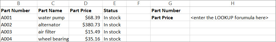
Use the LOOKUP function to search one row or one column. In the above example, we’re searching prices in column D.
Tips: Consider one of the newer lookup functions, depending on which version you are using.
-
Use VLOOKUP to search one row or column, or to search multiple rows and columns (like a table). It’s a much improved version of LOOKUP. Watch this video about how to use VLOOKUP.
-
If you are using Microsoft 365, use XLOOKUP — it’s not only faster, it also lets you search in any direction (up, down, left, right).
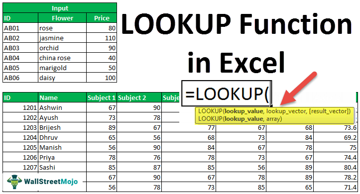
There are two ways to use LOOKUP: Vector form and Array form
-
Vector form: Use this form of LOOKUP to search one row or one column for a value. Use the vector form when you want to specify the range that contains the values that you want to match. For example, if you want to search for a value in column A, down to row 6.

-
Array form: We strongly recommend using VLOOKUP or HLOOKUP instead of the array form. Watch this video about using VLOOKUP. The array form is provided for compatibility with other spreadsheet programs, but it’s functionality is limited.
An array is a collection of values in rows and columns (like a table) that you want to search. For example, if you want to search columns A and B, down to row 6. LOOKUP will return the nearest match. To use the array form, your data must be sorted.
Vector form
The vector form of LOOKUP looks in a one-row or one-column range (known as a vector) for a value and returns a value from the same position in a second one-row or one-column range.
Syntax
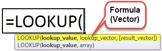
LOOKUP(lookup_value, lookup_vector, [result_vector])
The LOOKUP function vector form syntax has the following arguments:
-
lookup_value Required. A value that LOOKUP searches for in the first vector. Lookup_value can be a number, text, a logical value, or a name or reference that refers to a value.
-
lookup_vector Required. A range that contains only one row or one column. The values in lookup_vector can be text, numbers, or logical values.
Important: The values in lookup_vector must be placed in ascending order: …, -2, -1, 0, 1, 2, …, A-Z, FALSE, TRUE; otherwise, LOOKUP might not return the correct value. Uppercase and lowercase text are equivalent.
-
result_vector Optional. A range that contains only one row or column. The result_vector argument must be the same size as lookup_vector. It has to be the same size.
Remarks
-
If the LOOKUP function can’t find the lookup_value, the function matches the largest value in lookup_vector that is less than or equal to lookup_value.
-
If lookup_value is smaller than the smallest value in lookup_vector, LOOKUP returns the #N/A error value.
Vector examples
You can try out these examples in your own Excel worksheet to learn how the LOOKUP function works. In the first example, you’re going to end up with a spreadsheet that looks similar to this one:
-
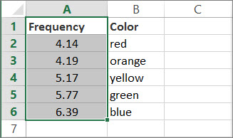
Copy the data in following table, and paste it into a new Excel worksheet.
Copy this data into column A
Copy this data into column B
Frequency
4.14
Color
red
4.19
orange
5.17
yellow
5.77
green
6.39
blue
-
Next, copy the LOOKUP formulas from the following table into column D of your worksheet.
Copy this formula into the D column
Here’s what this formula does
Here’s the result you’ll see
Formula
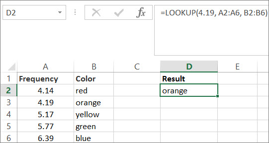
=LOOKUP(4.19, A2:A6, B2:B6)
Looks up 4.19 in column A, and returns the value from column B that is in the same row.
orange
=LOOKUP(5.75, A2:A6, B2:B6)
Looks up 5.75 in column A, matches the nearest smaller value (5.17), and returns the value from column B that is in the same row.
yellow
=LOOKUP(7.66, A2:A6, B2:B6)
Looks up 7.66 in column A, matches the nearest smaller value (6.39), and returns the value from column B that is in the same row.
blue
=LOOKUP(0, A2:A6, B2:B6)
Looks up 0 in column A, and returns an error because 0 is less than the smallest value (4.14) in column A.
#N/A
-
For these formulas to show results, you may need to select them in your Excel worksheet, press F2, and then press Enter. If you need to, adjust the column widths to see all the data.
Array form
The array form of LOOKUP looks in the first row or column of an array for the specified value and returns a value from the same position in the last row or column of the array. Use this form of LOOKUP when the values that you want to match are in the first row or column of the array.
Syntax
LOOKUP(lookup_value, array)
The LOOKUP function array form syntax has these arguments:
-
lookup_value Required. A value that LOOKUP searches for in an array. The lookup_value argument can be a number, text, a logical value, or a name or reference that refers to a value.
-
If LOOKUP can’t find the value of lookup_value, it uses the largest value in the array that is less than or equal to lookup_value.
-
If the value of lookup_value is smaller than the smallest value in the first row or column (depending on the array dimensions), LOOKUP returns the #N/A error value.
-
-
array Required. A range of cells that contains text, numbers, or logical values that you want to compare with lookup_value.
The array form of LOOKUP is very similar to the HLOOKUP and VLOOKUP functions. The difference is that HLOOKUP searches for the value of lookup_value in the first row, VLOOKUP searches in the first column, and LOOKUP searches according to the dimensions of array.
-
If array covers an area that is wider than it is tall (more columns than rows), LOOKUP searches for the value of lookup_value in the first row.
-
If an array is square or is taller than it is wide (more rows than columns), LOOKUP searches in the first column.
-
With the HLOOKUP and VLOOKUP functions, you can index down or across, but LOOKUP always selects the last value in the row or column.
Important: The values in array must be placed in ascending order: …, -2, -1, 0, 1, 2, …, A-Z, FALSE, TRUE; otherwise, LOOKUP might not return the correct value. Uppercase and lowercase text are equivalent.
-
На чтение 5 мин. Просмотров 1.6k. Опубликовано 25.06.2019
Функция Excel LOOKUP имеет две формы: векторную форму и форму массива .
Форма массива функции LOOKUP аналогична другим функциям поиска в Excel, таким как VLOOKUP и HLOOKUP, в том, что ее можно использовать для поиска или поиска определенных значений, расположенных в таблице данных.
Чем это отличается, так это:
- С помощью VLOOKUP и HLOOKUP вы можете выбрать, из какого столбца или строки возвращать значение данных, в то время как LOOKUP всегда возвращает значение из последней строки или столбца в массиве.
- При попытке найти совпадение для указанного значения – известного как Lookup_value – VLOOKUP выполняет поиск только в первом столбце данных, а HLOOKUP – только в первой строке, а функция LOOKUP – в первой строке или в столбце. в зависимости от формы массива.
Содержание
- Функция LOOKUP и форма массива
- Синтаксис и аргументы функции LOOKUP – форма массива
- Пример использования массива формы функции LOOKUP
- Сортировка данных
- Пример функции LOOKUP
- Ввод значения поиска
Функция LOOKUP и форма массива
Форма массива – будь то квадрат (равное количество столбцов и строк) или прямоугольник (неравное количество столбцов и строк) – влияет на то, где функция LOOKUP ищет данные:
- Если массив имеет квадратную форму или это высокий прямоугольник (выше его ширины), LOOKUP предполагает, что данные расположены в столбцах, и поэтому ищет совпадение с Lookup_value в первом столбец массива.
- Если массив является широким прямоугольником (шире его высоты), LOOKUP предполагает, что данные расположены в строках, и поэтому ищет совпадение с Lookup_value в первой строке массива.
Синтаксис и аргументы функции LOOKUP – форма массива

Синтаксис для формы массива функции LOOKUP:
= LOOKUP (Lookup_value, Array)
Lookup_value (обязательно) – значение, которое функция ищет в массиве. Значение Lookup_value может быть числом, текстом, логическим значением или ссылкой на имя или ячейку, которая ссылается на значение.
Массив (обязательно) – ячейки диапазона, в которых функция ищет значение Lookup_value. Данные могут быть текстовыми, числовыми или логическими значениями.
Для правильной работы функции LOOKUP аргумент Array должен быть отсортирован в порядке возрастания (от A до Z или от наименьшего к наибольшему для чисел)
Если функция не может найти точное соответствие для Lookup_value, она выбирает самое большое значение в массиве, которое меньше или равно значению Lookup_value
Если значение Lookup_value отсутствует или меньше всех значений в массиве, функция LOOKUP вернет ошибку # N/A
Пример использования массива формы функции LOOKUP
Как показано на рисунке выше, в этом примере будет использоваться форма массива функции LOOKUP, чтобы найти цену Whachamacallit в списке инвентаря.
Форма массива – высокий прямоугольник . Следовательно, функция вернет значение, расположенное в последнем столбце списка инвентаря.
Сортировка данных
Как указано в примечаниях выше, данные в массиве должны быть отсортированы в порядке возрастания, чтобы функция LOOKUP работала правильно.
При сортировке данных в Excel необходимо сначала выбрать столбцы и строки данных для сортировки. Обычно это включает в себя заголовки столбцов.
- Выделите ячейки от A4 до C10 на листе
- Нажмите на вкладку Данные в меню ленты.
- Нажмите на кнопку Сортировать в середине ленты, чтобы открыть диалоговое окно Сортировка
- Под заголовком Столбец в диалоговом окне выберите вариант сортировки по Деталь в раскрывающемся списке.
- При необходимости под заголовком Сортировать по выберите Значения в раскрывающемся списке.
- При необходимости под заголовком Заказ выберите А до Я в раскрывающемся списке.
- Нажмите ОК , чтобы отсортировать данные и закрыть диалоговое окно.
- Порядок данных теперь должен соответствовать указанному на рисунке выше.
Пример функции LOOKUP
Хотя можно просто набрать функцию LOOKUP
= LOOKUP (А2, А5: С10)
в ячейку рабочего листа многим людям проще использовать диалоговое окно функции.
Диалоговое окно позволяет вводить каждый аргумент в отдельной строке, не беспокоясь о синтаксисе функции – например, скобках и разделителях запятых между аргументами.
Следующие шаги подробно описывают, как функция LOOKUP была введена в ячейку B2 с помощью диалогового окна.
- Нажмите на ячейку B2 на рабочем листе, чтобы сделать ее активной;
- Нажмите на вкладку Формулы ;
- Выберите Поиск и ссылку на ленте, чтобы открыть раскрывающийся список функций;
- Нажмите на LOOKUP в списке, чтобы открыть диалоговое окно Выбрать аргументы ;
- Нажмите на lookup_value, array в списке;
- Нажмите ОК , чтобы открыть диалоговое окно Аргументы функций ;
- В диалоговом окне нажмите на строку Lookup_value ;
- Нажмите на ячейку A2 на рабочем листе, чтобы ввести ссылку на эту ячейку в диалоговое окно;
- Нажмите на строку Массив в диалоговом окне.
- Выделите ячейки от A5 до C10 на рабочем листе, чтобы ввести этот диапазон в диалоговое окно – этот диапазон содержит все данные, которые должны быть найдены функцией
- Нажмите ОК , чтобы завершить функцию и закрыть диалоговое окно.
- В ячейке E2 появляется ошибка # N/A , потому что нам еще предстоит ввести имя детали в ячейку D2
Ввод значения поиска
- Нажмите на ячейку A2, введите Whachamacallit и нажмите клавишу Enter на клавиатуре;
- Значение $ 23,56 должно появиться в ячейке B2, поскольку это цена Whachamacallit, расположенного в последнем столбце таблицы данных;
- Проверьте функцию, введя другие имена деталей в ячейку A2. Цена за каждую часть в списке появится в ячейке B2;
- При нажатии на ячейку E2 полная функция = LOOKUP (A2, A5: C10) появляется на панели формул над рабочим листом.
Use the LOOKUP function to look up a value in a one-column or one-row range, and retrieve a value from the same position in another one-column or one-row range. The lookup function has two forms, vector and array. The majority of this article describes the vector form, but the last example below illustrates the array form.
The LOOKUP function accepts three arguments: lookup_value, lookup_vector, and result_vector. The first argument, lookup_value, is the value to look for. The second argument, lookup_vector, is a one-row, or one-column range to search. LOOKUP assumes that lookup_vector is sorted in ascending order. The third argument, result_vector, is a one-row, or one-column range of results. Result_vector is optional. When result_vector is provided, LOOKUP locates a match in the lookup_vector, and returns the corresponding value from result_vector. If result_vector is not provided, LOOKUP returns the value of the match found in lookup_vector.
LOOKUP has default behaviors that make it useful when solving certain problems. For example, LOOKUP can be used to retrieve an approximate-matched value instead of a position and to find the last value in a row or column. LOOKUP assumes that values in lookup_vector are sorted in ascending order and always performs an approximate match. When LOOKUP can’t find a match, it will match the next smallest value.
Example #1 — basic usage
In the example shown above, the formula in cell F5 returns the value of the match found in column B. Note that result_vector is not provided:
=LOOKUP(F4,B5:B9) // returns match in level
The formula in cell F6 returns the corresponding Tier value from column C. Notice in this case, both lookup_vector and result_vector are provided:
=LOOKUP(F4,B5:B9,C5:C9) // returns corresponding tier
In both formulas, LOOKUP automatically performs an approximate match and it is therefore important that lookup_vector is sorted in ascending order.
Example #2 — last non-empty cell
LOOKUP can be used to get the value of the last filled (non-empty) cell in a column. In the screen below, the formula in F6 is:
=LOOKUP(2,1/(B:B<>""),B:B)

Note the use of a full column reference. This is not an intuitive formula, but it works well. The key to understanding this formula is to recognize that the lookup_value of 2 is deliberately larger than any values that will appear in the lookup_vector. Detailed explanation here.
Example #3 — latest price
Similar to the above example, the lookup function can be used to look up the latest price in data sorted in ascending order by date. In the screen below, the formula in G5 is:
=LOOKUP(2,1/(item=F5),price)
where item (B5:B12) and price (D5:D12) are named ranges.

When lookup_value is greater than all values in lookup_array, default behavior is to «fall back» to the previous value. This formula exploits this behavior by creating an array that contains only 1s and errors, then deliberately looking for the value 2, which will never be found. More details here.
Example #4 — array form
The LOOKUP function has an array form as well. In the array configuration, LOOKUP takes just two arguments: the lookup_value, and a single two-dimensional array:
LOOKUP(lookup_value, array) // array form
In the array form, LOOKUP evaluates the array and automatically changes behavior based on the array dimensions. If the array is wider than tall, LOOKUP looks for the lookup value in the first row of the array (like HLOOKUP). If the array is taller than wide (or square), LOOKUP looks for the lookup value in the first column (like VLOOKUP). In either case, LOOKUP returns a value at the same position from the last row or column in the array. The example below shows how the array form works. The formula in F5 is configured to use a vertical array and the formula in F6 is configured to use a horizontal array:
=LOOKUP(E5,B5:C9) // vertical array
=LOOKUP(E6,C11:G12) // horizontal array

The vertical and horizontal arrays contain the same values; only the orientation is different.
Note: Microsoft discourages the use of the array form and suggests VLOOKUP and HLOOKUP as better options.
Notes
- LOOKUP assumes that lookup_vector is sorted in ascending order.
- When lookup_value can’t be found, LOOKUP will match the next smallest value.
- When lookup_value is greater than all values in lookup_vector, LOOKUP matches the last value.
- When lookup_value is less than the first value in lookup_vector, LOOKUP returns #N/A.
- Result_vector must be the same size as lookup_vector.
- LOOKUP is not case-sensitive
sample files
1. ADDRESS Function
The ADDRESS Function returns a valid cell reference as per the column and row address. In simple words, you can create an address of a cell by using its row number and column number.
Syntax
ADDRESS(row_num,column_num,abs_num,A1,sheet_text)
Arguments
- row_num: A number to specify row number.
- column_num: A number to specify column number.
- [abs_num]: Reference type.
- [A1]: Reference style.
- [sheet_text]: A text value as a sheet name.
Notes
- By default, the ADDRESS function returns absolute reference in the result.
Example
In the below example, we have used different arguments to get all types of results.

With R1C1 reference style:
- Relative reference.
- Relative row and absolute column reference.
- Absolute row and relative column reference.
- Absolute reference.
With A1 reference style:
- Relative reference.
- Relative row and absolute column reference.
- Absolute row and relative column reference.
- Absolute reference.
2. AREAS Function
The AREAS Function returns a number that represents the number of ranges in the reference you have specified. In simple words, it actually counts the different worksheet areas you have referred to the function.
syntax
AREAS(reference)
Arguments
- reference: A Reference to a cell or a range of cells.
Notes
- Reference can be a cell, a range of cells or a named range.
- If you want to refer to more than one cell reference, you have to enclose all those references in more than one set of parentheses and use commas to separate each reference from others.
Example
In the below example, we have used areas function to get the number reference in a named range.

As you can see there are three columns in the range and it has returned 3 in the result.

3. CHOOSE Function
The CHOOSE function returns a value from the list of values based on the position number specified. In simple words, it looks for a value from a list based on its position and returns it in the result.
Syntax
CHOOSE(index_num,value1,value2,…)
Arguments
- index_num: A number for specifying the position of the value in the list.
- value1: A range of cells or an input value from which you can choose.
- [value2]: A range of cells or an input value from which you can choose.
Notes
- You can refer to a cell or you can also insert values directly in the function.
Example
In the below example, we have used CHOOSE function with a drop-down list to calculate four(sum, average, max, and mix) different things. So, we have used the below formula to calculate all four things:
=CHOOSE(VLOOKUP(K2,Q1:R4,2,FALSE),SUM(O2:O9),AVERAGE(O2:O9),MAX(O2:O9),MIN(O2:O9))

We have this small table with the name of all four calculations which we want and a serial number to each in the corresponding cell.
After that, we have a drop-down list for all four calculations. Now, to get index number in the choose function from that small table we have a lookup formula which will returns serial number as per the value selected from the drop-down list.
And instead of values, we have used four formulas for 4 different calculations.
4. COLUMN Function
The COLUMN function returns the column number for the given cell reference. As you know, every cell reference is made up of a column number and a row number. So it takes the column number and returns it in the result.
Syntax
COLUMN([reference])
Arguments
- reference: A cell reference for which you want to get the column number.
Notes
- You cannot refer to multiple references.
- If you refer to an array, the column function will also return the column numbers in an array.
- If you refer to a range of more than one cell, it will return the column number of the leftmost cell. For example, if you refer to the range A1:C10, it will return the column number of the cell A1.
- If you skip specifying a reference, it will return the column number of the current cell.
Example
In the below example, we have used COLUMN to get the column number of the cell A1.

As I have already mentioned, if you skip specifying cell reference it will return the column number of the current cell. In the below example, we have used COLUMN to create a header with serial numbers.

5. COLUMNS Function
The COLUMNS function returns the number of columns referred to in the given reference. In simple words, it counts how many columns are there in the supplied range and returns that count.
Syntax
COLUMNS(array)
Arguments
- array: An array or range of cells from which you want to get the number of columns.
Notes
- You can also use a named range.
- COLUMNS function is not concerned with the values in the cells, it will simply return the number of columns in a reference.
Example
In the below example, we have used COLUMN to get the number of columns from range A1:F1.

6. FORMULATEXT Function
The FORMULATEXT function returns the formula from the referred cell. And if there’s no formula in the referred cell, a value, or a blank, it will return a #N/A.
Syntax
FORMULATEXT(reference)
Arguments
- reference: The cell reference from which you want formula as a text.
Notes
- If you refer to another workbook that workbook should be open, otherwise it will not show the formula.
- If you refer to a range more than a single cell, it will return formula from the upper-left cell of the given range.
- It will return an “#N/A” error value if the cell you are using as a reference does not contain any formula, has a formula with more than 8192 characters, a cell is protected, or an external workbook is not opened.
- If you refer two cells in circular reference it will return results from both.
Example
In the below example, we have used formula text with different types of references. When you refer to a cell that doesn’t have any formula, it will return “#N/A” error value.

7. HLOOKUP Function
The HLOOKUP function lookups for a value in the top row of a table and returns the value from the same column of the matched value using the index number. In simple words, it performs a horizontal lookup.
Syntax
HLOOKUP(lookup_value, table_array, row_index_num, [range_lookup])
Arguments
- lookup_value: The value you want to lookup.
- table_array: The data table or an array from which you want to the lookup value.
- row_index_num: A numeric value representing a number of rows below from the top row from which you want the value. For example, if you specify 2 and your lookup value is in A10 in the data table, it will return value from cell B10.
- [range_lookup]: A logical value to specify the type of lookup. If you want to perform an exact match search use FALSE and if you want to perform a non-exact match use TRUE (Default).
Notes
- You can use wildcard characters.
- You can perform an exact match and an approximate match.
- While performing an approximate match make sure to sort data in ascending order from left to right, and if data is not in ascending order then it would return an inaccurate result.
- If range_lookup is true or omitted, it will perform a non-exact match but return an exact match if the lookup value exists in the lookup range.
- If range_lookup is true or omitted, and the lookup value is not in the lookup range, it will return the nearest value which is less than the lookup value.
- If range_lookup is false, then there is no need to sort data range.
Example
In the below example, we have used the HLOOKUP function with MATCH to create a dynamic formula and then we have used a drop-down list to change the lookup value from the cell.

The zone name from cell C7 is used as a lookup value. Range B1: F5 as table array and for row_index_num we have used match function to get the row number.

Whenever you change the value in cell C9, it will return the row number from the table array. You don’t have to change your formula again and again. Just change values with the drop-down list and you will get value for that.
8. HYPERLINK Function
The HYPERLINK function returns a string with a hyperlink attached to it. In simple words, like the HYPERLINK option you have in Excel, the HYPERLINK function helps you to create a hyperlink.
Syntax
HYPERLINK(link_location,[friendly_name])
Arguments
- Link_Location: The location for which you want to add a HYPERLINK. It can be further split into two terms.
- link: It can be an address of a cell or range of cells in the same worksheet or in any other worksheet or in any other workbook. We can also link a bookmark from a word document.
- location: It can be a link to a hard drive, a server using the UNC path, or any URL from the internet or intranet. (In Excel online you can only use web address for HYPERLINK function). You can insert a link to the function by inserting it as a text with quotation marks or by referring to a cell containing the link as a text. Make sure to use “HTTPS://” before a web address.
- [friendly_name]: It is an optional part of this function. It acts as the face of the connecting link.
- You can use any type of text, number, or both.
- You also refer to a cell which contains the friendly_name.
- If you skip it, the function will use the link address to display.
- If friendly_name returns an error, the function will display error.
Notes
- Link a file saved on a Web Address: You can use a file that is saved on a web address. This helps us to share the file in an effective way.
- Link a file saved on a Hard Drive: You can also use this function while working offline. You can link a file that is stored on your hard drive and access them through your single excel sheet, no need to go to every single folder to open them.
- Link a Word Document File: This is also an awesome feature of HYPERLINK function. You can link a Word document file or a specific place in word document file using a bookmark.
- Link a file without using Friendly Name: If you want to show the actual link to the file or place to the user. In this situation, you just need to skip the friendly name declaration in the HYPERLINK Function.
9. INDEX Function
The INDEX function returns a value from a list of values based on its index number. In simple words, INDEX returns a value from a list of values and you need to specify that value’s position.
Syntax
INDEX has two different syntaxes.
In the first, you can use an array form of an index to simply get a value from a list using its position.
INDEX(array, row_num, [column_num])
In the second, you can use a referral form that is less used in real life but you can use it if you have more than one range to get value from.
INDEX(reference, row_num, [column_num], [area_num])
Arguments
- array: A range of cells or an array constant.
- reference: A range of cells or multiple ranges.
- row_number: The number of the row from which you want to get the value.
- [col_number]: The number of the column from which you want to get the value.
- [area_number]: If you are referring to more than one range of cells (using reference syntax), specify a number to refer to a range from all those.
Notes
- When both the row_num and column_num arguments are specified, it will return the value in the cell at the intersection of both.
- If you specify row_num or column_num as 0 (zero), it will return the array of values for the entire column or row, respectively.
- When row_num and column_num are out the range, it will return an error #REF!.
- If area_number is greater than the number ranges you have specified then it will return #REF!.
Example
1. Using ARRAY – Getting Value from a List
In the below example, we have used the INDEX function to get the quantity of June month. In the list, Jun is in 6th position (6th row) that’s why I have specified 6 in row_number. INDEX has returned the value 1904 in the result.

And if you referring to a range with more than one column you have to specify the column number.
2. Using REFERENCE – Getting Value from Multiple Lists
In the below example, instead of selecting all the range in one go, I have selected it as three different ranges. In the last argument, we have specified 2 in area_number which will define the range to use from these three different ranges.

Now in the second range, we are referring to the 5th row and 1st column. INDEX has returned the value 172 which in the 5th row in the 2nd range.
10. INDIRECT Function
The INDIRECT function returns a valid reference from a text string which represents a cell reference. In simple words, you can refer to a cell range by using the cell address as a text value.
Syntax
INDIRECT(ref_text, [a1])
Arguments
- ref_text: A text which represents the address of a cell, an address of a range of cells, a named range, or a table name. For example, A1, B10:B20, or MyRange.
- [a1]: A number or a boolean value to represent the type of cell reference you are specifying in ref_text. For example, if you want to use A1 reference style use TRUE or 1 and if you want to use R1C1 reference style use FALSE or 0 for R1C reference style. And if you omit to specify the cell reference type, it will use A1 style as default.
Notes
- When you referred to another workbook, that workbook should be opened.
- If you insert a row or a column in the range which you have referred, INDIRECT will not update that reference.
- If you want to insert text directly into the function you have to put it in double quotation marks or you can also refer to a cell that has the text you want to use as a reference.
Example
1. Reference to Another Worksheet
You can also refer to another worksheet using the INDIRECT and you have to insert the worksheet name in it. In the below example, we have used the indirect function to refer to another worksheet and have the sheet name in cell A2 and cell reference in cell B2.

In cell C2, we have used the following formula to combine the text.
=INDIRECT(“‘”&A2&”‘!”&B2)
This combination creates a text which is used by the INDIRECT function to refer to the cell A1 in sheet1 and the best part is when you change the worksheet name or cell address the reference will automatically change.
Cell A1 in “Sheet1” has the value “Yes” and that’s why indirect returns the value “Yes”.
2. Reference to Another Workbook
You can also refer to another workbook, in the same way, we did for another worksheet. All you have to do, just add a workbook name in your text which you are using as a reference.

In the above example, we have used the following formula to get the value from the cell A1 of the workbook “Book1”.
=INDIRECT(“[“&A2&”]”&B2&”!”&C2)
As we have the workbook name in cell “A2”, worksheet name in cell “B2” and cell name in cell “C2”. We have combined them to use as an input text in indirect function.
Note: While combining cell reference as a text make sure to follow the right reference structure.
3. Using with Named Ranges
Yes, you can also refer to a named range using the indirect function. It’s just simple. Once you create a named range you have to enter that named range as a text in INDIRECT.

In the above example, we have a drop-down in cell E1 which has a list of named ranges, and in cell E2 we have used that name. As range B2:B5 is named as “Quantity” and range C2:C5 is named as “Amount”.
When you select quantity from drop-down indirect function instantly refers to the named range. And when you select the amount from the drop-down, you will have the sum of cell range C2:C5.
11. LOOKUP Function
The LOOKUP function returns a value (which you are looking up) from a row, column, or from an array. In simple words, you can look up for a value, and LOOKUP will return that value if it’s there in that row, column, or array.
Syntax
LOOKUP(value, lookup_range, [result_range])
There are two types of LOOKUP functions.
- Vector Form
- Array Form
Arguments
- value: The value that you want to search from a column or a row.
- lookup_range: The column or row from which you want to lookup for the value.
- [result_range]: The column or row from which you want to return a value. This is an optional argument.
Notes
- Instead of using array form it’s better to use VLOOKUP or HLOOKUP.
12. MATCH Function
The MATCH function returns the index number of the value from an array. In simple words, the MATCH function looks up for a value in the list and returns the position number of that value in the list.
Syntax
MATCH (lookup_value, lookup_array, [match_type])
Arguments
- lookup_value: The value whose position you want to get from a list of values.
- lookup_array: The range of cell or an array contains values.
- [match_type]: The number (-1, 0 & 1) to specify how excel look for the value from the list of values.
- If you use 1, it will return the largest value which is equal or less than the lookup value. The values in the list must be sorted in ascending order.
- If you use -1, it will return the smallest value which is equal or greater than the lookup value. The values in the list must be sorted in ascending order.
- If you use 0, it will return the exact match from the list.
Notes
- You can use wildcard characters.
- If there is no matching value in the list if will return #N/A.
- The match function is non-case sensitive.
Example
In the below example, we have used 1 as match type and we are looking for value 5.

As I have already mentioned if you use 1 in match type it returns the largest value which is equal or smaller than the lookup value. In the entire list, there are 3 values that are smaller than 5 and 4 is the highest in them.
That’s why in the result it has returned 3 which is the position of value 4.
13. OFFSET Function
The OFFSET function returns a reference to a range which is a specific number of rows and columns away from a cell or range of cells. In simple words, you can refer to a cell or a range of cells by using rows and columns from a starting cell.
Syntax
OFFSET(reference, rows, cols, [height], [width])
Arguments
- reference: The reference from which you want to offset to start. It can be a cell or range of adjacent cells.
- rows: The number of rows that tell OFFSET to move up or down from the reference. To go downward you need a positive number and for going upwards you need a negative number.
- cols: The number of columns tells OFFSET to move to the left or right from the reference. To go right you need a positive number and for going left you need a negative number.
- [height]: A number to specify the rows to include in the reference.
- [width]: A number to specify the columns to include in the reference.
Notes
- OFFSET is a “volatile” function, it recalculates whenever there is any change to a worksheet.
- It displays the #REF! error value if the offset is outside the edge of the worksheet.
- If height or width is omitted, the height and width of reference are used.
Example
In the below example, we have used SUM with OFFSET to create a dynamic range which sums the values from all the months for a particular product.

14. ROW Function
The ROW function returns the row number of the referred cell. In simple words, with the ROW function, you can get the row number of a cell and if you don’t refer to any cell then it returns the row number for the cell where you insert it.
Syntax
ROW([reference])
Arguments
- reference: A cell reference or a range of cells for which you want to check the row number.
Notes
- It will include all types of sheets (Chart Sheet, Worksheet or Macro Sheet).
- You can refer to sheets even if they are visible, hidden or very hidden.
- If you skip specifying any value in the function it will give you the sheet number of the sheet in which you have applied the function.
- If you specify an invalid sheet name, it will return a #N/A.
- If you specify an invalid sheet reference, it will return a #REF!.
Example
In the below example, we have used the row function check the row number of the same cell where we have used the function.

In the below example, we have referred to another cell to get the row number of that cell.

You can use the row function to create a serial number list in your worksheet. All you have to do is just enter row functions in a cell and drag it up to the cell you want to add serial numbers.

15. ROWS Function
The ROWS function returns a count of the rows from the referred range. In simple words, with the ROWS function you can count how many rows are in the range you have referred to.
Syntax
ROWS(array)
Arguments
- array: A cell reference or an array to check the number of rows.
Notes
- You can also use a named range.
- It is not concerned with the values in the cells, it will simply return the number of rows in a reference.
Example
In the below example, we have referred to a vertical range of 10 cells and it has returned 10 in the result as the range includes 10 rows.

16. TRANSPOSE Function
The TRANSPOSE function changes the orientation of a range. In simple words, by using this function you can change the data from a row into a column and from a column into a row.
Syntax
TRANSPOSE (array)
Arguments
- array: An array or a range you want to transpose.
Notes
- You have to apply TRANSPOSE as an array function, using the same number of cells as you have in your source range by pressing Ctrl + Shift + Enter.
- If you select cells less than source range, it will transpose data only for those cells.
Example
Here we need to transpose data from range B2:D4 to range G2 to I4:

For this, first, we need to go to the cell G2 and select cell range up to I4.

Next is to enter (=TRANSPOSE(B2:D4)) in cell G2 and press Ctrl+Shift+Enter.

TRANSPOSE will convert the data from the rows into columns, and the formula which we have applied is an array formula, you cannot change a single cell from it.

17. VLOOKUP Function
The VLOOKUP function lookups for a value in the first column of a table and returns the value from the same row of the matched value using the index number. In simple words, it performs a vertical lookup.
Syntax
VLOOKUP(lookup_value,table_array,col_index_num,range_lookup)
Arguments
- lookup_value: A value that you want to search in a column. You can refer to a cell that has the lookup value or you can directly enter that value into the function.
- table_array: A range of cells, a named range from which you want to look up the value.
- col_index_num: A number represents the column number from which you want to retrieve the value.
- range_lookup: Use false or 0 to make an exact match and true or 1 for an appropriate match. The default is True.
Notes
- If VLOOKUP cannot find the value you are looking for, it will return an #N/A.
- VLOOKUP is only able to give you the value which is on the right side of the lookup value. If you want to look upon the right side, you can use INDEX and MATCH for that.
- If you are using an exact match then it will only match the value which is first in the column.
- You can also use wildcard characters with VLOOKUP.
- You can use TRUE or 1 if you want an appropriate match and FALSE or 0 for an exact match.
- If you are using an appropriate match (True): It will return the next smallest value from the list if there is no exact match.
- If the value which you are looking for is smaller than the smallest value in the list, VLOOKUP will return #N/A.
- If there is an exact value exists which you are looking for, it will give you that exact value.
- Make sure you have sorted the list in ascending order.
Example
1. Using VLOOKUP for Categories
In the below example, we have a list of students with marks they have scored, and in the remarks column, we want to a grade according to their marks.

In the above marks list, we want to add remarks as per the below category range.

In this, we have two options to use.
FIRST is to create a nesting formula with IF which is a little bit time-consuming, and the SECOND option is to create a formula with VLOOKUP with an appropriate match. And, the formula will be:
=VLOOKUP(B2,$E$2:$G$5,3,TRUE)

How it works
I am using the “MIN MARKS” column to match the lookup value and I am getting value in return from the “Remarks” column.
I have already mentioned that when you use TRUE and there is no exact match lookup value then it will return the next smallest value from the lookup value. For example, when we are looking for a value 77 from the category table, 65 is the next smallest value after 77.
That is why we got “Good” in remarks.
2. Handling Errors in VLOOKUP Function
One of the most common problems which come when you are using VLOOKUP is that you’ll get #N/A whenever there is no match is found by it. But the solution to this problem is simple and easy. Let me show with an easy example.
In the below example, we have a list of names and their age and in cell E6, we are using the VLOOKUP function to look up a name from the list. Whenever I type a name that is not on the list I am getting #N/A.

But what I want here is to show a meaningful message instead of the error. The formula will be: =IFNA(VLOOKUP(D6,Sheet3!$A$1:$B$14,2,0),”Not Found”)

How it works: IFNA can test a value for #N/A and if there is an error you can specify a value instead of the error.
The LOOKUP excel function searches a value in a range (single row or single column) and returns a corresponding match from the same position of another range (single row or single column). The corresponding match is a piece of information associated with the value being searched.
For example, the branch code (search value) can be used to retrieve the profits of different bank branches (corresponding match). Being a lookup and reference function, the LOOKUP has two varieties–vector and array.
The VLOOKUPThe VLOOKUP excel function searches for a particular value and returns a corresponding match based on a unique identifier. A unique identifier is uniquely associated with all the records of the database. For instance, employee ID, student roll number, customer contact number, seller email address, etc., are unique identifiers.
read more and HLOOKUPHlookup is a referencing worksheet function that finds and matches the value from a row rather than a column using a reference. Hlookup stands for horizontal lookup, in which we search for data in rows horizontally.read more are improved versions of the LOOKUP function.
The LOOKUP is different from the VLOOKUP function in the sense that the former looks for a match in a one-row or one-column range while the latter searches the entire data table.
Table of contents
- What is LOOKUP Excel Function?
- LOOKUP Excel Function–Syntax 1 (Vector Form)
- LOOKUP Excel Function–Syntax 2 (Array Form)
- The Explanation of the LOOKUP Function
- How to use the LOOKUP Function in Excel?
- Example #1–Vector Form
- Example #2–Vector Form
- Example #3–Vector Form
- Example #4–Array Form
- Applications
- Frequently Asked Questions
- LOOKUP Excel Video
- Recommended Articles
LOOKUP Excel Function–Syntax 1 (Vector Form)
In the present context, a one-row or one-column range is known as a vector. In this form, the function searches a particular value in one vector and returns a corresponding value at the same position from another vector.
The syntax of the vector form is shown in the following image:
The function accepts the following arguments in the vector form:
- Lookup_value: This is the value to be searched.
- Lookup_vector: This is the one-row or one-column range in which the value is to be searched. It should be sorted in alphabetical order or ascending order to obtain correct results.
- Result_vector: This is the one-row or one-column range from which the output is to be returned. The output returned is in the same position as the “lookup_value.”
The “lookup_value” and “lookup_vector” are mandatory arguments while “result_vector” is optional.
Note: The “lookup_vector” and the “result_vector” both are one-row or one-column range with the same size. If the latter is omitted, Excel returns a value from the former.
LOOKUP Excel Function–Syntax 2 (Array Form)
In this form, the function searches a specified value in the first row or column of the array and returns a corresponding value at the same position from the last row or column of the array.
The syntax of the array form is shown in the following image:

The function accepts the following mandatory arguments in the array form:
- Lookup_value: This is the value to be searched.
- Array: This is the array or range where the value is to be searched.
The first row or column of the array is similar to the “lookup_vector” (vector form). The last row or column of the array is similar to the “result_vector” (vector form).
The Explanation of the LOOKUP Function
The LOOKUP function works on a close match or an approximate match. The two forms of the function are explained in the current section.
The Vector Form
The LOOKUP function looks for the exact “lookup_value” in the “lookup_vector” and returns the output at the same position from the “result_vector.” The possibilities are stated as follows:
- If the function does not find an exact match, it looks up the largest value in the “lookup_vector,” which is less than or equal to the “lookup_value.”
- If the “lookup_value” is smaller than all the values of the “lookup_vector,” the function returns “#N/A error”.
- If the “lookup_value” is greater than all the values of the “lookup_vector,” the function matches with the last value of the array.
- If the “lookup_value” occurs multiple times in the “lookup_vector,” the function considers the last occurrence of the former.
The “lookup_value,” “lookup_vector,” and “result_vector” can be a number, text string, date, currency, and so on.
The Array Form
The LOOKUP function searches for a value according to the dimensions (size) of the array. The possibilities are stated as follows:
- If the number of rows is more than the columns (column size is greater than or equal to the row size), the function searches for the “lookup_value” in the first column.
- If the number of columns is more than the rows (row size is greater than the column size), the function searches for the “lookup_value” in the first row.
You are free to use this image on your website, templates, etc, Please provide us with an attribution linkArticle Link to be Hyperlinked
For eg:
Source: LOOKUP Excel Function (wallstreetmojo.com)
How to use the LOOKUP Function in Excel?
Let us understand the working of the LOOKUP function with the help of examples.
You can download this LOOKUP Function Excel Template here – LOOKUP Function Excel Template
Example #1–Vector Form
The succeeding table shows a list of flowers, the identifier (ID), and the current price. The output to be retrieved with the help of the LOOKUP function is stated as follows:
a. The price of the flower given its ID
b. The price of the flower given its name
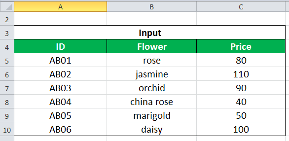
a. We use the following syntax for extracting the price of the flower with its ID.
“=LOOKUP(ID_to_search,A5:A10,C5:C10)”
Since the value to be searched can be supplied as a cell reference, enter E5 in the formula. This is shown in the succeeding image.
“=LOOKUP(E5,A5:A10,C5:C10)”
The formula returns 50.

b. We use the following formula for extracting the price of the flower with its name.
“=LOOKUP(“orchid”,B5:B10,C5:C10)”
The formula returns 90.
Example #2–Vector Form
The following table displays the transaction costs (in dollars) incurred on various dates beginning from January 2009. The output to be retrieved with the help of the LOOKUP function is stated as follows:
a. The cost of the last transaction of 2012
b. The cost of the last transaction of March

a. We use the following formula for extracting information on the last transaction of 2012.
“=LOOKUP(D4,YEAR(A4:A18),B4:B18)”
The “YEAR(A4:A18)” retrieves the year from the dates given in A4:A18. Since D4=2012, the formula returns $40000.

b. We use the following formula for extracting the cost of the last transaction of March.
“=LOOKUP(3,MONTH(A4:A18),B4:B18)”
The “MONTH(A4:A18)” extracts the month from the dates given in A4:A18. The formula returns $110000.
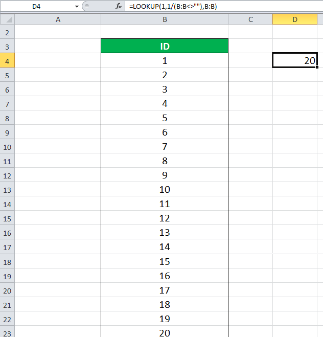
Example #3–Vector Form
The following table shows a list of IDs in column B. We want to retrieve the last entry of the column with the help of the LOOKUP function. The situations for retrieval are stated as follows:
a. When IDs are listed from 1 to 10
b. When IDs are listed from 1 to 20

a. We use the following formula to extract the last entry of column B.
“=LOOKUP(1,1/(B:B<>””),B:B)”
In the formula, the “lookup_value” is 1, the “lookup_vector” is 1/(B:B<>””), and the “result_vector” is B:B.
The (B:B<>””) forms an array of “true” and “false” where the former means a value is present, while the latter means it is absent. This array is divided by 1 to form another array of “1” and “0” which corresponds to “true” and “false” respectively.
Since the “lookup_value” is 1, the LOOKUP function looks for 1 in the array of “1” and “0.” It matches the “lookup_value” with the last “1” and returns a corresponding match. In this case, the corresponding match is the actual “lookup_value” at the same position, which is 10.
The output of the formula is 10, as shown in the following image.

b. We use the same formula (explained in the preceding section) to extract the last entry of column B.
“=LOOKUP(1,1/(B:B<>””),B:B)”
The formula returns 20, as shown in the following image.
Example #4–Array Form
The following table (B3:I24) shows the roll numbers (ID), names of the students, marks in five subjects, and average marks. We want to retrieve the average marks with the help of the student ID.
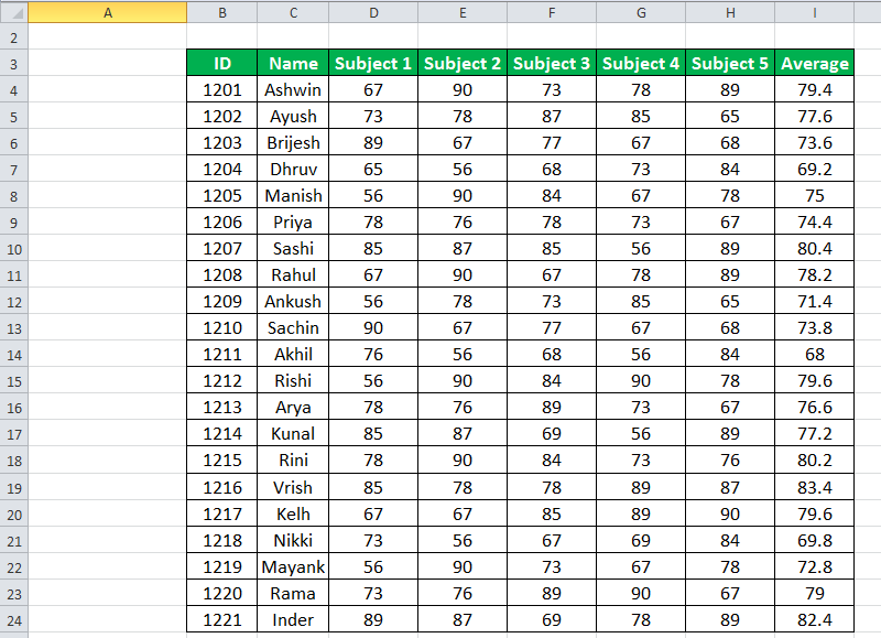
Since the ID to look for is in cell K4, the following formula is used.
“=LOOKUP(K4,B4:I24)”
The formula returns the corresponding average marks of the student Dhruv (ID 1204). The output is 69.2, as shown in the following image.
Applications
The function is used in the following situations:
- To extract the price of an item using its identifier
- To find the location of a book in the library
- To obtain the last transaction cost for a given month or year
- To check the latest price of a product
- To find the last row within a range of numerical or textual data
- To retrieve the last transaction date
Note: The LOOKUP function of Excel is not case-sensitive implying that it treats the uppercase and lowercase letters the same.
Frequently Asked Questions
Define the LOOKUP function of Excel.
The LOOKUP function looks for a value in a single row or column and returns a corresponding value having the same position from another row or column. The look up and the extraction data both should be a one-row or a one-column range.
The LOOKUP function of Excel has two forms which are explained as follows:
• Vector form–The “lookup_value” is searched in the “lookup_vector” and a corresponding match is returned from the “result_vector.” The syntax is stated as follows:
“LOOKUP(lookup_value,lookup_vector,[result_vector])”
The first two arguments are mandatory and the last one is optional.
• Array form–The “lookup_value” is searched in the first row or column of the “array” and a corresponding match is returned from the last row or column of the “array.” The syntax is stated as follows:
“LOOKUP(lookup_value,array)”
Both the arguments are mandatory.
When should the LOOKUP function of Excel be used?
The usage of the general LOOKUP function, the vector, and the array forms is mentioned as follows:
• The general function is used when there is a need to retrieve an associated piece of information from a one-row or a one-column range.
• The vector form is used when there is a need to specify the range from which a corresponding match is to be returned.
• The array form is used when the lookup or search value is in the first row or column and the corresponding match is in the last row or column.
Note: It is recommended to use the VLOOKUP and HLOOKUP as an alternative to the array form.
What is the difference between the LOOKUP, VLOOKUP, and HLOOKUP functions of Excel?
The differences between the three functions are stated as follows:
• The LOOKUP searches for a value in a one-row or one-column range. In contrast, the VLOOKUP and HLOOKUP search for a value in two or more columns or rows respectively.
• The array form of the LOOKUP searches the “lookup_value” according to the dimensions of the array. In comparison, the VLOOKUP and the HLOOKUP search for the “lookup_value” in the first column and the first row respectively.
• The LOOKUP looks for an approximate match while the VLOOKUP and HLOOKUP work for both approximate and exact matches.
• The LOOKUP has cross functionality implying that it is capable of performing both vertical and horizontal lookups. On the other hand, the VLOOKUP and HLOOKUP are limited to only vertical and horizontal lookups respectively.
LOOKUP Excel Video
Recommended Articles
This has been a tutorial to LOOKUP Excel function. Here we discuss how to use LOOKUP formula along with step by step practical examples. You can download the Excel template from the website. You may also go through these useful functions in Excel-
- Power BI VlookupVLOOKUP in Power BI helps the users fetch data from the other tables. Since it is not an inbuilt function, the user needs to replicate it using the DAX function like the LOOKUPVALUE DAX function.read more
- VBA LOOKUPLOOKUP is the function to fetch the data from the main table based on a single lookup value. VBA LOOKUP function doesn’t require a data structure like that. It doesn’t matter whether the result column is to the right or left. It can fetch the data comfortably.read more
- Excel VLOOKUP FormulaThe VLOOKUP excel function searches for a particular value and returns a corresponding match based on a unique identifier. A unique identifier is uniquely associated with all the records of the database. For instance, employee ID, student roll number, customer contact number, seller email address, etc., are unique identifiers.
read more - Degrees Function in ExcelDEGREES function in excel is used to convert the angles mentioned in radians which are determined based on the radius of a circle to degrees. It is one of the mathematical and trigonometric functions inbuilt into Excel to resolve the problem with radians.read more
- Excel TroubleshootingTroubleshooting in Excel helps when we tend to get some errors or unexpected results associated with the formula we use in Excel. read more
![]()
Download Article
![]()
Download Article
Whenever you keep track of data in spreadsheets, there’ll come a time when you want to find information without having to scroll through endless columns or rows. We’ll show you how to use Microsoft Excel’s LOOKUP function to find a value from one row or column in a different row or column. If you’re looking to do a reverse Vlookup, check out How to Do a Reverse Vlookup in Google Sheets.
Steps
-
1
Create a two column list toward the bottom of the page. In this example, one column has numbers and the other has random words.
-
2
Decide on cell that you would like the user to select from, this is where a drop down list will be.
Advertisement
-
3
Once you click on the cell, the border should darken, select the DATA tab on the tool bar, then select VALIDATION.
-
4
A pop up should appear, in the ALLOW list pick LIST.
-
5
Now to pick your source, in other words your first column, select the button with the red arrow.
-
6
Select the first column of your list and press enter and click OK when the data validation window appears, now you should see a box with an arrow on, if you click on it your list should drop down.
-
7
Select another box where you want the other information to show up.
-
8
Once you clicked that box, go to the INSERT tab and FUNCTION.
-
9
Once the box pops up, select LOOKUP & REFERENCE from the category list.
-
10
Find LOOKUP in the list and double-click it, another box should appear click OK.
-
11
For the lookup_value select the cell with the drop down list.
-
12
For the Lookup_vector select the first column of your list.
-
13
For the Result_vector select the second column.
-
14
Now whenever you pick something from the drop down list the info should automatically change.


Advertisement
Ask a Question
200 characters left
Include your email address to get a message when this question is answered.
Submit
Advertisement
Video
-
Whenever you are completed you can change the font color to white, to make the list hidden.
-
Save your work constantly, especially if the list is extensive
-
Make sure when you are in the DATA VALIDATION window (Step 5) the box labeled IN-CELL DROPDOWN is checked
Show More Tips
Thanks for submitting a tip for review!
Advertisement
About This Article
Thanks to all authors for creating a page that has been read 312,656 times.
Is this article up to date?
This Excel tutorial explains how to use the Excel LOOKUP function with syntax and examples.
Description
The Microsoft Excel LOOKUP function returns a value from a range (one row or one column) or from an array.
The LOOKUP function is a built-in function in Excel that is categorized as a Lookup/Reference Function. It can be used as a worksheet function (WS) in Excel. As a worksheet function, the LOOKUP function can be entered as part of a formula in a cell of a worksheet.
There are 2 different syntaxes for the LOOKUP function:
LOOKUP Function (Syntax #1)
In Syntax #1, the LOOKUP function searches for value in the lookup_range and returns the value in the result_range that is in the same position.
The syntax for the LOOKUP function in Microsoft Excel is:
LOOKUP( value, lookup_range, [result_range] )
Parameters or Arguments
- value
- The value to search for in the lookup_range.
- lookup_range
- A single row or single column of data that is sorted in ascending order. The LOOKUP function searches for value in this range.
- result_range
- Optional. It is a single row or single column of data that is the same size as the lookup_range. The LOOKUP function searches for the value in the lookup_range and returns the value from the same position in the result_range. If this parameter is omitted, it will return the first column of data.
Returns
The LOOKUP function returns any datatype such as a string, numeric, date, etc.
If the LOOKUP function can not find an exact match, it chooses the largest value in the lookup_range that is less than or equal to the value.
If the value is smaller than all of the values in the lookup_range, then the LOOKUP function will return #N/A.
If the values in the LOOKUP_range are not sorted in ascending order, the LOOKUP function will return the incorrect value.
Example (as Worksheet Function)
Let’s look at some Excel LOOKUP function examples and explore how to use the LOOKUP function as a worksheet function in Microsoft Excel:
Based on the Excel spreadsheet above, the following LOOKUP examples would return:
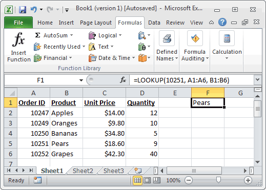
=LOOKUP(10251, A1:A6, B1:B6)
Result: "Pears"

=LOOKUP(10251, A1:A6)
Result: 10251

=LOOKUP(10246, A1:A6, B1:B6)
Result: #N/A

=LOOKUP(10248, A1:A6, B1:B6)
Result: "Apples"
LOOKUP Function (Syntax #2)
In Syntax #2, the LOOKUP function searches for the value in the first row or column of the array and returns the corresponding value in the last row or column of the array.
The syntax for the LOOKUP function in Microsoft Excel is:
LOOKUP( value, array )
Parameters or Arguments
- value
- The value to search for in the array. The values must be in ascending order.
- array
- An array of values that contains both the values to search for and return.
Returns
The LOOKUP function returns any datatype such as a string, numeric, date, etc.
If the LOOKUP function can not find an exact match, it chooses the largest value in the lookup_range that is less than or equal to the value.
If the value is smaller than all of the values in the lookup_range, then the LOOKUP function will return #N/A.
If the values in the array are not sorted in ascending order, the LOOKUP function will return the incorrect value.
Example (as Worksheet Function)
Let’s look at some Excel LOOKUP function examples and explore how to use the LOOKUP function as a worksheet function in Microsoft Excel:
=LOOKUP("T", {"s","t","u","v";10,11,12,13})
Result: 11

=LOOKUP("Tech on the Net", {"s","t","u","v";10,11,12,13})
Result: 11

=LOOKUP("t", {"s","t","u","v";"a","b","c","d"})
Result: "b"

=LOOKUP("r", {"s","t","u","v";"a","b","c","d"})
Result: #N/A

=LOOKUP(2, {1,2,3,4;511,512,513,514})
Result: 512
Frequently Asked Questions
Question: In Microsoft Excel, I have a table of data in cells A2:D5. I’ve tried to create a simple LOOKUP to find CB2 in the data, but it always returns 0. What am I doing wrong?
Answer: Using the LOOKUP function can sometimes be a bit tricky so let’s look at an example. Below we have a spreadsheet with the data that you described.
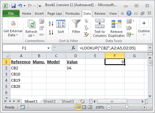
In cell F1, we’ve placed the following formula:
=LOOKUP("CB2",A2:A5,D2:D5)
And yes, even though CB2 exists in the data, the LOOKUP function returns 0.
Now, let’s explain what is happening. At first, it looks like the function isn’t finding CB2 in the list, but in fact, it is finding something else. Let’s fill in the empty cells in D3:D5 to explain better.
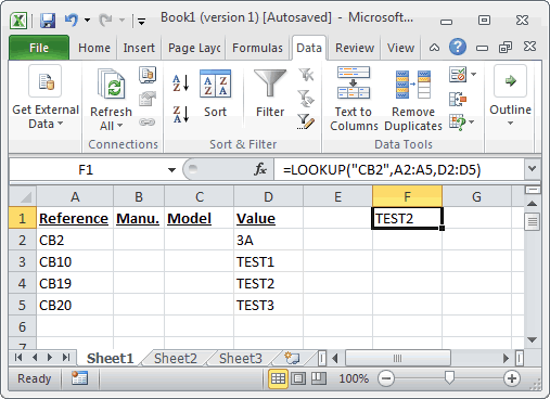
If we place the values TEST1, TEST2, TEST3 in cells D3, D4, 5, respectively, we can see that the LOOKUP function is in fact returning the value TEST2. So we ask ourselves, when we are looking up CB2 in the data and CB2 exists in the data, why is it returning the value for CB19? Good question. The LOOKUP function assumes that the data in column A is sorted in ascending order.
If you look closer at column A, it is not in fact sorted in ascending order. If we quickly sorted column A, it would look like this:
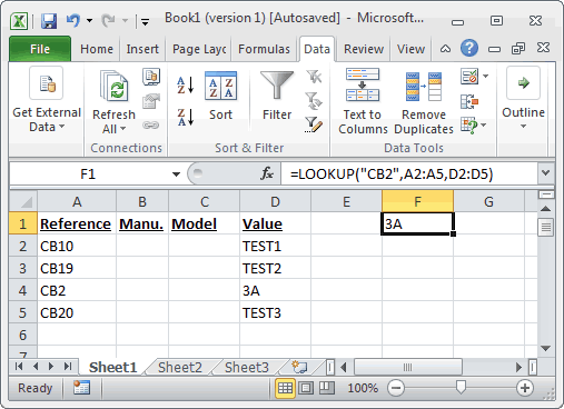
Now the LOOKUP function correctly returns 3A when it is looking up CB2 in the data.
To avoid these sorting problems with your data, we recommend using VLOOKUP function in this case. Let’s show you how we would do this. If we changed our formula below (but left our data in column A in the original sort order):
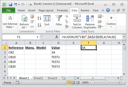
The following VLOOKUP formula would return the correct value of 3A.
=VLOOKUP("CB2",$A$2:$D$5,4,FALSE)
The VLOOKUP function does not require us to have the data sorted in ascending order since we used FALSE as the last parameter — which means that it is looking for an exact match.
Question: I have the following LOOKUP formula:
=LOOKUP(C2,{"A","B","C","D","E","F","G","H","I","K","X","Z"}, {"1","2","3","4","5","6","7","8","9","10","12","1"})
I also need to add zero to the lookup vector and result vector. How do I do this?
Answer: Using numbers in Excel can be tricky, as you can enter them either as numeric or text values. Because of this, there are 2 possible solutions.
Numeric Solution
If you have entered your zero as a numeric value, then the following formula will work:
=LOOKUP(C2,{0,"A","B","C","D","E","F","G","H","I","K","X","Z"}, {0,"1","2","3","4","5","6","7","8","9","10","12","1"})
Text Solution
If you have entered your zero as a text value, then the following formula will work:
=LOOKUP(C2,{"0","A","B","C","D","E","F","G","H","I","K","X","Z"}, {"0","1","2","3","4","5","6","7","8","9","10","12","1"})
Question: For the following function in Microsoft Excel:
=LOOKUP(M14,Sheet2!A2:A2240,Sheet2!B2:B2240)
How do I get it to return a blank cell if the LOOKUP value (M14) is blank?
Answer: To check for a blank value in cell M14, you can use the IF function and ISBLANK function as follows:
=IF(ISBLANK(M14),"",LOOKUP(M14,Sheet2!A2:A2240,Sheet2!B2:B2240))
Now if the value in cell M14 is blank, the formula will return a blank. Otherwise it will perform the LOOKUP function as before.