Use LOOKUP, one of the lookup and reference functions, when you need to look in a single row or column and find a value from the same position in a second row or column.
For example, let’s say you know the part number for an auto part, but you don’t know the price. You can use the LOOKUP function to return the price in cell H2 when you enter the auto part number in cell H1.
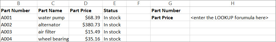
Use the LOOKUP function to search one row or one column. In the above example, we’re searching prices in column D.
Tips: Consider one of the newer lookup functions, depending on which version you are using.
-
Use VLOOKUP to search one row or column, or to search multiple rows and columns (like a table). It’s a much improved version of LOOKUP. Watch this video about how to use VLOOKUP.
-
If you are using Microsoft 365, use XLOOKUP — it’s not only faster, it also lets you search in any direction (up, down, left, right).
There are two ways to use LOOKUP: Vector form and Array form
-
Vector form: Use this form of LOOKUP to search one row or one column for a value. Use the vector form when you want to specify the range that contains the values that you want to match. For example, if you want to search for a value in column A, down to row 6.

-
Array form: We strongly recommend using VLOOKUP or HLOOKUP instead of the array form. Watch this video about using VLOOKUP. The array form is provided for compatibility with other spreadsheet programs, but it’s functionality is limited.
An array is a collection of values in rows and columns (like a table) that you want to search. For example, if you want to search columns A and B, down to row 6. LOOKUP will return the nearest match. To use the array form, your data must be sorted.
Vector form
The vector form of LOOKUP looks in a one-row or one-column range (known as a vector) for a value and returns a value from the same position in a second one-row or one-column range.
Syntax
LOOKUP(lookup_value, lookup_vector, [result_vector])
The LOOKUP function vector form syntax has the following arguments:
-
lookup_value Required. A value that LOOKUP searches for in the first vector. Lookup_value can be a number, text, a logical value, or a name or reference that refers to a value.
-
lookup_vector Required. A range that contains only one row or one column. The values in lookup_vector can be text, numbers, or logical values.
Important: The values in lookup_vector must be placed in ascending order: …, -2, -1, 0, 1, 2, …, A-Z, FALSE, TRUE; otherwise, LOOKUP might not return the correct value. Uppercase and lowercase text are equivalent.
-
result_vector Optional. A range that contains only one row or column. The result_vector argument must be the same size as lookup_vector. It has to be the same size.
Remarks
-
If the LOOKUP function can’t find the lookup_value, the function matches the largest value in lookup_vector that is less than or equal to lookup_value.
-
If lookup_value is smaller than the smallest value in lookup_vector, LOOKUP returns the #N/A error value.
Vector examples
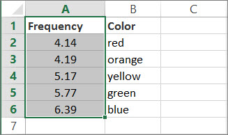
You can try out these examples in your own Excel worksheet to learn how the LOOKUP function works. In the first example, you’re going to end up with a spreadsheet that looks similar to this one:
-
Copy the data in following table, and paste it into a new Excel worksheet.
Copy this data into column A
Copy this data into column B
Frequency
4.14
Color
red
4.19
orange
5.17
yellow
5.77
green
6.39
blue
-
Next, copy the LOOKUP formulas from the following table into column D of your worksheet.
Copy this formula into the D column
Here’s what this formula does
Here’s the result you’ll see
Formula
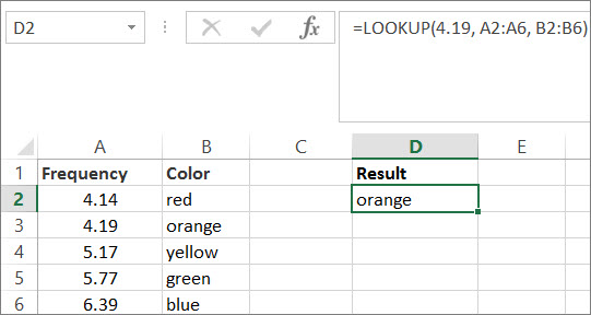
=LOOKUP(4.19, A2:A6, B2:B6)
Looks up 4.19 in column A, and returns the value from column B that is in the same row.
orange
=LOOKUP(5.75, A2:A6, B2:B6)
Looks up 5.75 in column A, matches the nearest smaller value (5.17), and returns the value from column B that is in the same row.
yellow
=LOOKUP(7.66, A2:A6, B2:B6)
Looks up 7.66 in column A, matches the nearest smaller value (6.39), and returns the value from column B that is in the same row.
blue
=LOOKUP(0, A2:A6, B2:B6)
Looks up 0 in column A, and returns an error because 0 is less than the smallest value (4.14) in column A.
#N/A
-
For these formulas to show results, you may need to select them in your Excel worksheet, press F2, and then press Enter. If you need to, adjust the column widths to see all the data.
Array form
The array form of LOOKUP looks in the first row or column of an array for the specified value and returns a value from the same position in the last row or column of the array. Use this form of LOOKUP when the values that you want to match are in the first row or column of the array.
Syntax
LOOKUP(lookup_value, array)
The LOOKUP function array form syntax has these arguments:
-
lookup_value Required. A value that LOOKUP searches for in an array. The lookup_value argument can be a number, text, a logical value, or a name or reference that refers to a value.
-
If LOOKUP can’t find the value of lookup_value, it uses the largest value in the array that is less than or equal to lookup_value.
-
If the value of lookup_value is smaller than the smallest value in the first row or column (depending on the array dimensions), LOOKUP returns the #N/A error value.
-
-
array Required. A range of cells that contains text, numbers, or logical values that you want to compare with lookup_value.
The array form of LOOKUP is very similar to the HLOOKUP and VLOOKUP functions. The difference is that HLOOKUP searches for the value of lookup_value in the first row, VLOOKUP searches in the first column, and LOOKUP searches according to the dimensions of array.
-
If array covers an area that is wider than it is tall (more columns than rows), LOOKUP searches for the value of lookup_value in the first row.
-
If an array is square or is taller than it is wide (more rows than columns), LOOKUP searches in the first column.
-
With the HLOOKUP and VLOOKUP functions, you can index down or across, but LOOKUP always selects the last value in the row or column.
Important: The values in array must be placed in ascending order: …, -2, -1, 0, 1, 2, …, A-Z, FALSE, TRUE; otherwise, LOOKUP might not return the correct value. Uppercase and lowercase text are equivalent.
-
Содержание
- Check if a cell contains text (case-insensitive)
- Find cells that contain text
- Check if a cell has any text in it
- Check if a cell matches specific text
- Check if part of a cell matches specific text
- Find or replace text and numbers on a worksheet
- Replace
- Use Excel built-in functions to find data in a table or a range of cells
- Summary
- Create the Sample Worksheet
- Term Definitions
- Functions
- LOOKUP()
- VLOOKUP()
- INDEX() and MATCH()
- OFFSET() and MATCH()
- Search For Text in Excel
- How to Search For Text in Excel?
- Which Formula Can Tell Us A Cell Contains Specific Text?
- Alternatives to FIND Function
- Alternative #1 – Excel Search Function
- Alternative #2 – Excel Countif Function
- Highlight the Cell which has a Particular Text Value
- Recommended Articles
Check if a cell contains text (case-insensitive)
Let’s say you want to ensure that a column contains text, not numbers. Or, perhapsyou want to find all orders that correspond to a specific salesperson. If you have no concern for upper- or lowercase text, there are several ways to check if a cell contains text.
You can also use a filter to find text. For more information, see Filter data.
Find cells that contain text
Follow these steps to locate cells containing specific text:
Select the range of cells that you want to search.
To search the entire worksheet, click any cell.
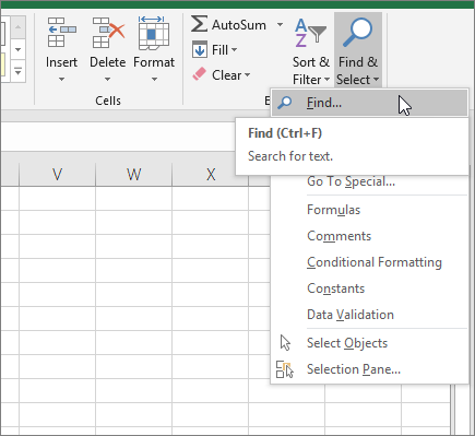
On the Home tab, in the Editing group, click Find & Select, and then click Find.
In the Find what box, enter the text—or numbers—that you need to find. Or, choose a recent search from the Find what drop-down box.
Note: You can use wildcard characters in your search criteria.
To specify a format for your search, click Format and make your selections in the Find Format popup window.
Click Options to further define your search. For example, you can search for all of the cells that contain the same kind of data, such as formulas.
In the Within box, you can select Sheet or Workbook to search a worksheet or an entire workbook.
Click Find All or Find Next.
Find All lists every occurrence of the item that you need to find, and allows you to make a cell active by selecting a specific occurrence. You can sort the results of a Find All search by clicking a header.
Note: To cancel a search in progress, press ESC.
Check if a cell has any text in it
To do this task, use the ISTEXT function.
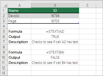
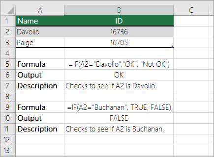
Check if a cell matches specific text
Use the IF function to return results for the condition that you specify.
Check if part of a cell matches specific text
To do this task, use the IF, SEARCH, and ISNUMBER functions.
Note: The SEARCH function is case-insensitive.
Источник
Find or replace text and numbers on a worksheet

Use the Find and Replace features in Excel to search for something in your workbook, such as a particular number or text string. You can either locate the search item for reference, or you can replace it with something else. You can include wildcard characters such as question marks, tildes, and asterisks, or numbers in your search terms. You can search by rows and columns, search within comments or values, and search within worksheets or entire workbooks.
Tip: You can also use formulas to replace text. Check out the SUBSTITUTE function or REPLACE, REPLACEB functions to learn more.

To find something, press Ctrl+F, or go to Home > Editing > Find & Select > Find.
Note: In the following example, we’ve clicked the Options >> button to show the entire Find dialog. By default, it will display with Options hidden.

In the Find what: box, type the text or numbers you want to find, or click the arrow in the Find what: box, and then select a recent search item from the list.
Tips: You can use wildcard characters — question mark ( ?), asterisk ( *), tilde (
) — in your search criteria.
Use the question mark (?) to find any single character — for example, s?t finds «sat» and «set».
Use the asterisk (*) to find any number of characters — for example, s*d finds «sad» and «started».
) followed by ?, *, or
to find question marks, asterisks, or other tilde characters — for example, fy91
Click Find All or Find Next to run your search.
Tip: When you click Find All, every occurrence of the criteria that you are searching for will be listed, and clicking a specific occurrence in the list will select its cell. You can sort the results of a Find All search by clicking a column heading.
Click Options>> to further define your search if needed:
Within: To search for data in a worksheet or in an entire workbook, select Sheet or Workbook.
Search: You can choose to search either By Rows (default), or By Columns.
Look in: To search for data with specific details, in the box, click Formulas, Values, Notes, or Comments.
Note: Formulas, Values, Notes and Comments are only available on the Find tab; only Formulas are available on the Replace tab.
Match case — Check this if you want to search for case-sensitive data.
Match entire cell contents — Check this if you want to search for cells that contain just the characters that you typed in the Find what: box.
If you want to search for text or numbers with specific formatting, click Format, and then make your selections in the Find Format dialog box.
Tip: If you want to find cells that just match a specific format, you can delete any criteria in the Find what box, and then select a specific cell format as an example. Click the arrow next to Format, click Choose Format From Cell, and then click the cell that has the formatting that you want to search for.
Replace
To replace text or numbers, press Ctrl+H, or go to Home > Editing > Find & Select > Replace.
Note: In the following example, we’ve clicked the Options >> button to show the entire Find dialog. By default, it will display with Options hidden.

In the Find what: box, type the text or numbers you want to find, or click the arrow in the Find what: box, and then select a recent search item from the list.
Tips: You can use wildcard characters — question mark ( ?), asterisk ( *), tilde (
) — in your search criteria.
Use the question mark (?) to find any single character — for example, s?t finds «sat» and «set».
Use the asterisk (*) to find any number of characters — for example, s*d finds «sad» and «started».
) followed by ?, *, or
to find question marks, asterisks, or other tilde characters — for example, fy91
In the Replace with: box, enter the text or numbers you want to use to replace the search text.
Click Replace All or Replace.
Tip: When you click Replace All, every occurrence of the criteria that you are searching for will be replaced, while Replace will update one occurrence at a time.
Click Options>> to further define your search if needed:
Within: To search for data in a worksheet or in an entire workbook, select Sheet or Workbook.
Search: You can choose to search either By Rows (default), or By Columns.
Look in: To search for data with specific details, in the box, click Formulas, Values, Notes, or Comments.
Note: Formulas, Values, Notes and Comments are only available on the Find tab; only Formulas are available on the Replace tab.
Match case — Check this if you want to search for case-sensitive data.
Match entire cell contents — Check this if you want to search for cells that contain just the characters that you typed in the Find what: box.
If you want to search for text or numbers with specific formatting, click Format, and then make your selections in the Find Format dialog box.
Tip: If you want to find cells that just match a specific format, you can delete any criteria in the Find what box, and then select a specific cell format as an example. Click the arrow next to Format, click Choose Format From Cell, and then click the cell that has the formatting that you want to search for.
There are two distinct methods for finding or replacing text or numbers on the Mac. The first is to use the Find & Replace dialog. The second is to use the Search bar in the ribbon.
Источник
Use Excel built-in functions to find data in a table or a range of cells
Summary
This step-by-step article describes how to find data in a table (or range of cells) by using various built-in functions in Microsoft Excel. You can use different formulas to get the same result.
Create the Sample Worksheet
This article uses a sample worksheet to illustrate Excel built-in functions. Consider the example of referencing a name from column A and returning the age of that person from column C. To create this worksheet, enter the following data into a blank Excel worksheet.
You will type the value that you want to find into cell E2. You can type the formula in any blank cell in the same worksheet.
Term Definitions
This article uses the following terms to describe the Excel built-in functions:
The whole lookup table
The value to be found in the first column of Table_Array.
Lookup_Array
-or-
Lookup_Vector
The range of cells that contains possible lookup values.
The column number in Table_Array the matching value should be returned for.
3 (third column in Table_Array)
Result_Array
-or-
Result_Vector
A range that contains only one row or column. It must be the same size as Lookup_Array or Lookup_Vector.
A logical value (TRUE or FALSE). If TRUE or omitted, an approximate match is returned. If FALSE, it will look for an exact match.
This is the reference from which you want to base the offset. Top_Cell must refer to a cell or range of adjacent cells. Otherwise, OFFSET returns the #VALUE! error value.
This is the number of columns, to the left or right, that you want the upper-left cell of the result to refer to. For example, «5» as the Offset_Col argument specifies that the upper-left cell in the reference is five columns to the right of reference. Offset_Col can be positive (which means to the right of the starting reference) or negative (which means to the left of the starting reference).
Functions
LOOKUP()
The LOOKUP function finds a value in a single row or column and matches it with a value in the same position in a different row or column.
The following is an example of LOOKUP formula syntax:
The following formula finds Mary’s age in the sample worksheet:
The formula uses the value «Mary» in cell E2 and finds «Mary» in the lookup vector (column A). The formula then matches the value in the same row in the result vector (column C). Because «Mary» is in row 4, LOOKUP returns the value from row 4 in column C (22).
NOTE: The LOOKUP function requires that the table be sorted.
For more information about the LOOKUP function, click the following article number to view the article in the Microsoft Knowledge Base:
VLOOKUP()
The VLOOKUP or Vertical Lookup function is used when data is listed in columns. This function searches for a value in the left-most column and matches it with data in a specified column in the same row. You can use VLOOKUP to find data in a sorted or unsorted table. The following example uses a table with unsorted data.
The following is an example of VLOOKUP formula syntax:
The following formula finds Mary’s age in the sample worksheet:
The formula uses the value «Mary» in cell E2 and finds «Mary» in the left-most column (column A). The formula then matches the value in the same row in Column_Index. This example uses «3» as the Column_Index (column C). Because «Mary» is in row 4, VLOOKUP returns the value from row 4 in column C (22).
For more information about the VLOOKUP function, click the following article number to view the article in the Microsoft Knowledge Base:
INDEX() and MATCH()
You can use the INDEX and MATCH functions together to get the same results as using LOOKUP or VLOOKUP.
The following is an example of the syntax that combines INDEX and MATCH to produce the same results as LOOKUP and VLOOKUP in the previous examples:
The following formula finds Mary’s age in the sample worksheet:
The formula uses the value «Mary» in cell E2 and finds «Mary» in column A. It then matches the value in the same row in column C. Because «Mary» is in row 4, the formula returns the value from row 4 in column C (22).
NOTE: If none of the cells in Lookup_Array match Lookup_Value («Mary»), this formula will return #N/A.
For more information about the INDEX function, click the following article number to view the article in the Microsoft Knowledge Base:
OFFSET() and MATCH()
You can use the OFFSET and MATCH functions together to produce the same results as the functions in the previous example.
The following is an example of syntax that combines OFFSET and MATCH to produce the same results as LOOKUP and VLOOKUP:
This formula finds Mary’s age in the sample worksheet:
The formula uses the value «Mary» in cell E2 and finds «Mary» in column A. The formula then matches the value in the same row but two columns to the right (column C). Because «Mary» is in column A, the formula returns the value in row 4 in column C (22).
For more information about the OFFSET function, click the following article number to view the article in the Microsoft Knowledge Base:
Источник
Search For Text in Excel


How to Search For Text in Excel?
When working with Excel, we see so many peculiar situations. One of those situations is searching for the particular text in the cell. The first thing that comes to mind when we say we want to search for a specific text in the worksheet is the “Find and Replace” method in Excel, which is the most popular one. But Ctrl + F can find the text you are looking for but cannot go beyond that. So, for example, if the cell contains certain words, you may want the result in the next cell as “TRUE” or “FALSE.” So, Ctrl + F stops there.
Table of contents
You are free to use this image on your website, templates, etc., Please provide us with an attribution link How to Provide Attribution? Article Link to be Hyperlinked
For eg:
Source: Search For Text in Excel (wallstreetmojo.com)
Here, we will take you through the formulas to search for the particular text in the cell value and arrive at the result.
Which Formula Can Tell Us A Cell Contains Specific Text?
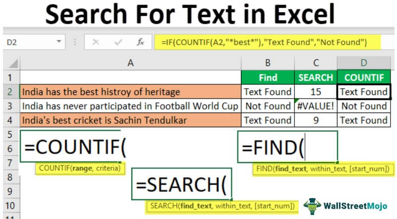
It is a question we have seen many times in Excel forums. The first formula that came to mind was the “FIND” function.
The FIND function can return the position of the supplied text values in the string. So, if the FIND method returns any number, then we can consider the cell as it has the text or else not.
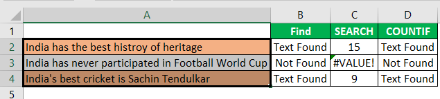
- For example, look at the below data.
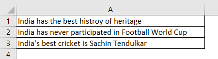
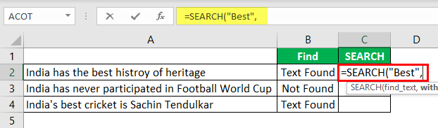
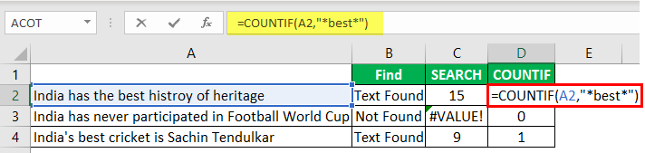
In the above data, we have three sentences in three different rows. Now in each cell, we need to search for the text “Best.” So, apply the FIND function.

The “find_text” argument mentions the text we need to find.

For the “within_text,” select the full sentence, i.e., cell reference.

The last parameter is not required to close the bracket and press the “Enter” key.

So, in two sentences, we have the word “best.” We can see the error value of #VALUE! in cell B2, which shows that cell A2 does not have the text value “best.”
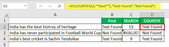
Instead of numbers, we can also enter the result in our own words. For this, we need to use the IF condition.
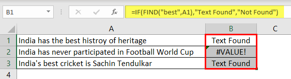
So, in the IF condition, we have supplied the result as “Text Found” if the value “best” is found. Otherwise, we have provided the result as “Not Found.”
But, here we have a problem, even though we have supplied the result as “Not Found,” if the text is still not found, we are getting the error value as #VALUE!.
So, nobody wants to have an error value in their Excel sheet. Therefore, we must enclose the formula with the ISNUMERIC function to overcome this error value.

The ISNUMERIC function evaluates whether the FIND function returns the number or not. If the FIND function returns the number, it will supply TRUE to the IF condition or else FALSE condition. Based on the result provided by the ISNUMERIC function, the IF condition will return the result accordingly.
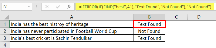
We can also use the IFERROR function in excel IFERROR Function In Excel The IFERROR function in Excel checks a formula (or a cell) for errors and returns a specified value in place of the error. read more to deal with error values instead of ISNUMERIC. For example, the below formula will also return “Not Found” if the FIND function returns the error value.
Alternatives to FIND Function
Alternative #1 – Excel Search Function
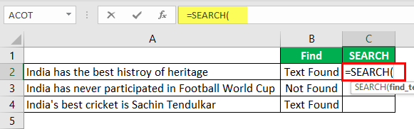
Supply the “find_text” as “Best.”
The “within_text” is our cell reference.
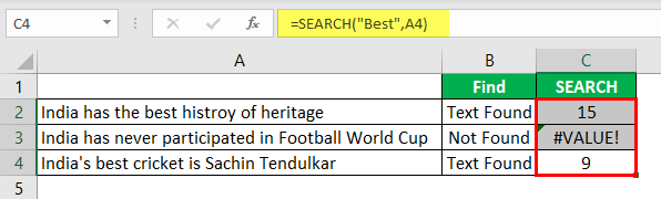
Even the SEARCH function returns an error value as #VALUE! If the finding text “best” is not found. As we have seen above, we need to enclose the formula with ISNUMERIC or IFERROR functions.
Alternative #2 – Excel Countif Function
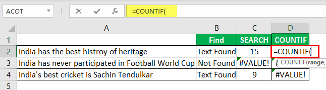
In the range, the argument selects the cell reference.
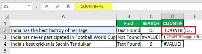
This formula will return the word “best” count in the selected cell value. Since we have only one “best” value, we will get only 1 as the count.
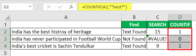
We can apply only the IF condition to get the result without error.
Highlight the Cell which has a Particular Text Value
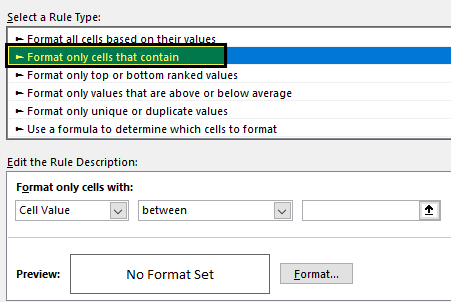
First, select the data cells and click “Conditional Formatting” > “New Rule.”
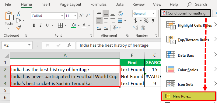
Under “New Rule,” select the “Format only cells that contain” option.
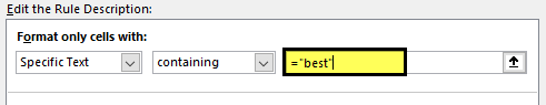
From the first dropdown, select “Specific Text.”

The formula section enters the text we search for in double quotes with the equal sign. =’best.’
Then, click on “FORMAT” and choose the formatting style.
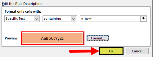
Click on “OK.” It will highlight all the cells which have the word “best.”
Using various techniques, we can search the particular text in Excel.
Recommended Articles
This article is a guide to Search For Text in Excel. Here, we discuss the top three methods to search the cell value for a specific text and arrive at the result with practical examples and a downloadable Excel template. You may learn more about Excel from the following articles: –
Источник
sample files
1. ADDRESS Function
The ADDRESS Function returns a valid cell reference as per the column and row address. In simple words, you can create an address of a cell by using its row number and column number.
Syntax
ADDRESS(row_num,column_num,abs_num,A1,sheet_text)
Arguments
- row_num: A number to specify row number.
- column_num: A number to specify column number.
- [abs_num]: Reference type.
- [A1]: Reference style.
- [sheet_text]: A text value as a sheet name.
Notes
- By default, the ADDRESS function returns absolute reference in the result.
Example
In the below example, we have used different arguments to get all types of results.

With R1C1 reference style:
- Relative reference.
- Relative row and absolute column reference.
- Absolute row and relative column reference.
- Absolute reference.
With A1 reference style:
- Relative reference.
- Relative row and absolute column reference.
- Absolute row and relative column reference.
- Absolute reference.
2. AREAS Function
The AREAS Function returns a number that represents the number of ranges in the reference you have specified. In simple words, it actually counts the different worksheet areas you have referred to the function.
syntax
AREAS(reference)
Arguments
- reference: A Reference to a cell or a range of cells.
Notes
- Reference can be a cell, a range of cells or a named range.
- If you want to refer to more than one cell reference, you have to enclose all those references in more than one set of parentheses and use commas to separate each reference from others.
Example
In the below example, we have used areas function to get the number reference in a named range.

As you can see there are three columns in the range and it has returned 3 in the result.

3. CHOOSE Function
The CHOOSE function returns a value from the list of values based on the position number specified. In simple words, it looks for a value from a list based on its position and returns it in the result.
Syntax
CHOOSE(index_num,value1,value2,…)
Arguments
- index_num: A number for specifying the position of the value in the list.
- value1: A range of cells or an input value from which you can choose.
- [value2]: A range of cells or an input value from which you can choose.
Notes
- You can refer to a cell or you can also insert values directly in the function.
Example
In the below example, we have used CHOOSE function with a drop-down list to calculate four(sum, average, max, and mix) different things. So, we have used the below formula to calculate all four things:
=CHOOSE(VLOOKUP(K2,Q1:R4,2,FALSE),SUM(O2:O9),AVERAGE(O2:O9),MAX(O2:O9),MIN(O2:O9))

We have this small table with the name of all four calculations which we want and a serial number to each in the corresponding cell.
After that, we have a drop-down list for all four calculations. Now, to get index number in the choose function from that small table we have a lookup formula which will returns serial number as per the value selected from the drop-down list.
And instead of values, we have used four formulas for 4 different calculations.
4. COLUMN Function
The COLUMN function returns the column number for the given cell reference. As you know, every cell reference is made up of a column number and a row number. So it takes the column number and returns it in the result.
Syntax
COLUMN([reference])
Arguments
- reference: A cell reference for which you want to get the column number.
Notes
- You cannot refer to multiple references.
- If you refer to an array, the column function will also return the column numbers in an array.
- If you refer to a range of more than one cell, it will return the column number of the leftmost cell. For example, if you refer to the range A1:C10, it will return the column number of the cell A1.
- If you skip specifying a reference, it will return the column number of the current cell.
Example
In the below example, we have used COLUMN to get the column number of the cell A1.

As I have already mentioned, if you skip specifying cell reference it will return the column number of the current cell. In the below example, we have used COLUMN to create a header with serial numbers.

5. COLUMNS Function
The COLUMNS function returns the number of columns referred to in the given reference. In simple words, it counts how many columns are there in the supplied range and returns that count.
Syntax
COLUMNS(array)
Arguments
- array: An array or range of cells from which you want to get the number of columns.
Notes
- You can also use a named range.
- COLUMNS function is not concerned with the values in the cells, it will simply return the number of columns in a reference.
Example
In the below example, we have used COLUMN to get the number of columns from range A1:F1.

6. FORMULATEXT Function
The FORMULATEXT function returns the formula from the referred cell. And if there’s no formula in the referred cell, a value, or a blank, it will return a #N/A.
Syntax
FORMULATEXT(reference)
Arguments
- reference: The cell reference from which you want formula as a text.
Notes
- If you refer to another workbook that workbook should be open, otherwise it will not show the formula.
- If you refer to a range more than a single cell, it will return formula from the upper-left cell of the given range.
- It will return an “#N/A” error value if the cell you are using as a reference does not contain any formula, has a formula with more than 8192 characters, a cell is protected, or an external workbook is not opened.
- If you refer two cells in circular reference it will return results from both.
Example
In the below example, we have used formula text with different types of references. When you refer to a cell that doesn’t have any formula, it will return “#N/A” error value.

7. HLOOKUP Function
The HLOOKUP function lookups for a value in the top row of a table and returns the value from the same column of the matched value using the index number. In simple words, it performs a horizontal lookup.
Syntax
HLOOKUP(lookup_value, table_array, row_index_num, [range_lookup])
Arguments
- lookup_value: The value you want to lookup.
- table_array: The data table or an array from which you want to the lookup value.
- row_index_num: A numeric value representing a number of rows below from the top row from which you want the value. For example, if you specify 2 and your lookup value is in A10 in the data table, it will return value from cell B10.
- [range_lookup]: A logical value to specify the type of lookup. If you want to perform an exact match search use FALSE and if you want to perform a non-exact match use TRUE (Default).
Notes
- You can use wildcard characters.
- You can perform an exact match and an approximate match.
- While performing an approximate match make sure to sort data in ascending order from left to right, and if data is not in ascending order then it would return an inaccurate result.
- If range_lookup is true or omitted, it will perform a non-exact match but return an exact match if the lookup value exists in the lookup range.
- If range_lookup is true or omitted, and the lookup value is not in the lookup range, it will return the nearest value which is less than the lookup value.
- If range_lookup is false, then there is no need to sort data range.
Example
In the below example, we have used the HLOOKUP function with MATCH to create a dynamic formula and then we have used a drop-down list to change the lookup value from the cell.

The zone name from cell C7 is used as a lookup value. Range B1: F5 as table array and for row_index_num we have used match function to get the row number.

Whenever you change the value in cell C9, it will return the row number from the table array. You don’t have to change your formula again and again. Just change values with the drop-down list and you will get value for that.
8. HYPERLINK Function
The HYPERLINK function returns a string with a hyperlink attached to it. In simple words, like the HYPERLINK option you have in Excel, the HYPERLINK function helps you to create a hyperlink.
Syntax
HYPERLINK(link_location,[friendly_name])
Arguments
- Link_Location: The location for which you want to add a HYPERLINK. It can be further split into two terms.
- link: It can be an address of a cell or range of cells in the same worksheet or in any other worksheet or in any other workbook. We can also link a bookmark from a word document.
- location: It can be a link to a hard drive, a server using the UNC path, or any URL from the internet or intranet. (In Excel online you can only use web address for HYPERLINK function). You can insert a link to the function by inserting it as a text with quotation marks or by referring to a cell containing the link as a text. Make sure to use “HTTPS://” before a web address.
- [friendly_name]: It is an optional part of this function. It acts as the face of the connecting link.
- You can use any type of text, number, or both.
- You also refer to a cell which contains the friendly_name.
- If you skip it, the function will use the link address to display.
- If friendly_name returns an error, the function will display error.
Notes
- Link a file saved on a Web Address: You can use a file that is saved on a web address. This helps us to share the file in an effective way.
- Link a file saved on a Hard Drive: You can also use this function while working offline. You can link a file that is stored on your hard drive and access them through your single excel sheet, no need to go to every single folder to open them.
- Link a Word Document File: This is also an awesome feature of HYPERLINK function. You can link a Word document file or a specific place in word document file using a bookmark.
- Link a file without using Friendly Name: If you want to show the actual link to the file or place to the user. In this situation, you just need to skip the friendly name declaration in the HYPERLINK Function.
9. INDEX Function
The INDEX function returns a value from a list of values based on its index number. In simple words, INDEX returns a value from a list of values and you need to specify that value’s position.
Syntax
INDEX has two different syntaxes.
In the first, you can use an array form of an index to simply get a value from a list using its position.
INDEX(array, row_num, [column_num])
In the second, you can use a referral form that is less used in real life but you can use it if you have more than one range to get value from.
INDEX(reference, row_num, [column_num], [area_num])
Arguments
- array: A range of cells or an array constant.
- reference: A range of cells or multiple ranges.
- row_number: The number of the row from which you want to get the value.
- [col_number]: The number of the column from which you want to get the value.
- [area_number]: If you are referring to more than one range of cells (using reference syntax), specify a number to refer to a range from all those.
Notes
- When both the row_num and column_num arguments are specified, it will return the value in the cell at the intersection of both.
- If you specify row_num or column_num as 0 (zero), it will return the array of values for the entire column or row, respectively.
- When row_num and column_num are out the range, it will return an error #REF!.
- If area_number is greater than the number ranges you have specified then it will return #REF!.
Example
1. Using ARRAY – Getting Value from a List
In the below example, we have used the INDEX function to get the quantity of June month. In the list, Jun is in 6th position (6th row) that’s why I have specified 6 in row_number. INDEX has returned the value 1904 in the result.

And if you referring to a range with more than one column you have to specify the column number.
2. Using REFERENCE – Getting Value from Multiple Lists
In the below example, instead of selecting all the range in one go, I have selected it as three different ranges. In the last argument, we have specified 2 in area_number which will define the range to use from these three different ranges.

Now in the second range, we are referring to the 5th row and 1st column. INDEX has returned the value 172 which in the 5th row in the 2nd range.
10. INDIRECT Function
The INDIRECT function returns a valid reference from a text string which represents a cell reference. In simple words, you can refer to a cell range by using the cell address as a text value.
Syntax
INDIRECT(ref_text, [a1])
Arguments
- ref_text: A text which represents the address of a cell, an address of a range of cells, a named range, or a table name. For example, A1, B10:B20, or MyRange.
- [a1]: A number or a boolean value to represent the type of cell reference you are specifying in ref_text. For example, if you want to use A1 reference style use TRUE or 1 and if you want to use R1C1 reference style use FALSE or 0 for R1C reference style. And if you omit to specify the cell reference type, it will use A1 style as default.
Notes
- When you referred to another workbook, that workbook should be opened.
- If you insert a row or a column in the range which you have referred, INDIRECT will not update that reference.
- If you want to insert text directly into the function you have to put it in double quotation marks or you can also refer to a cell that has the text you want to use as a reference.
Example
1. Reference to Another Worksheet
You can also refer to another worksheet using the INDIRECT and you have to insert the worksheet name in it. In the below example, we have used the indirect function to refer to another worksheet and have the sheet name in cell A2 and cell reference in cell B2.

In cell C2, we have used the following formula to combine the text.
=INDIRECT(“‘”&A2&”‘!”&B2)
This combination creates a text which is used by the INDIRECT function to refer to the cell A1 in sheet1 and the best part is when you change the worksheet name or cell address the reference will automatically change.
Cell A1 in “Sheet1” has the value “Yes” and that’s why indirect returns the value “Yes”.
2. Reference to Another Workbook
You can also refer to another workbook, in the same way, we did for another worksheet. All you have to do, just add a workbook name in your text which you are using as a reference.

In the above example, we have used the following formula to get the value from the cell A1 of the workbook “Book1”.
=INDIRECT(“[“&A2&”]”&B2&”!”&C2)
As we have the workbook name in cell “A2”, worksheet name in cell “B2” and cell name in cell “C2”. We have combined them to use as an input text in indirect function.
Note: While combining cell reference as a text make sure to follow the right reference structure.
3. Using with Named Ranges
Yes, you can also refer to a named range using the indirect function. It’s just simple. Once you create a named range you have to enter that named range as a text in INDIRECT.

In the above example, we have a drop-down in cell E1 which has a list of named ranges, and in cell E2 we have used that name. As range B2:B5 is named as “Quantity” and range C2:C5 is named as “Amount”.
When you select quantity from drop-down indirect function instantly refers to the named range. And when you select the amount from the drop-down, you will have the sum of cell range C2:C5.
11. LOOKUP Function
The LOOKUP function returns a value (which you are looking up) from a row, column, or from an array. In simple words, you can look up for a value, and LOOKUP will return that value if it’s there in that row, column, or array.
Syntax
LOOKUP(value, lookup_range, [result_range])
There are two types of LOOKUP functions.
- Vector Form
- Array Form
Arguments
- value: The value that you want to search from a column or a row.
- lookup_range: The column or row from which you want to lookup for the value.
- [result_range]: The column or row from which you want to return a value. This is an optional argument.
Notes
- Instead of using array form it’s better to use VLOOKUP or HLOOKUP.
12. MATCH Function
The MATCH function returns the index number of the value from an array. In simple words, the MATCH function looks up for a value in the list and returns the position number of that value in the list.
Syntax
MATCH (lookup_value, lookup_array, [match_type])
Arguments
- lookup_value: The value whose position you want to get from a list of values.
- lookup_array: The range of cell or an array contains values.
- [match_type]: The number (-1, 0 & 1) to specify how excel look for the value from the list of values.
- If you use 1, it will return the largest value which is equal or less than the lookup value. The values in the list must be sorted in ascending order.
- If you use -1, it will return the smallest value which is equal or greater than the lookup value. The values in the list must be sorted in ascending order.
- If you use 0, it will return the exact match from the list.
Notes
- You can use wildcard characters.
- If there is no matching value in the list if will return #N/A.
- The match function is non-case sensitive.
Example
In the below example, we have used 1 as match type and we are looking for value 5.

As I have already mentioned if you use 1 in match type it returns the largest value which is equal or smaller than the lookup value. In the entire list, there are 3 values that are smaller than 5 and 4 is the highest in them.
That’s why in the result it has returned 3 which is the position of value 4.
13. OFFSET Function
The OFFSET function returns a reference to a range which is a specific number of rows and columns away from a cell or range of cells. In simple words, you can refer to a cell or a range of cells by using rows and columns from a starting cell.
Syntax
OFFSET(reference, rows, cols, [height], [width])
Arguments
- reference: The reference from which you want to offset to start. It can be a cell or range of adjacent cells.
- rows: The number of rows that tell OFFSET to move up or down from the reference. To go downward you need a positive number and for going upwards you need a negative number.
- cols: The number of columns tells OFFSET to move to the left or right from the reference. To go right you need a positive number and for going left you need a negative number.
- [height]: A number to specify the rows to include in the reference.
- [width]: A number to specify the columns to include in the reference.
Notes
- OFFSET is a “volatile” function, it recalculates whenever there is any change to a worksheet.
- It displays the #REF! error value if the offset is outside the edge of the worksheet.
- If height or width is omitted, the height and width of reference are used.
Example
In the below example, we have used SUM with OFFSET to create a dynamic range which sums the values from all the months for a particular product.

14. ROW Function
The ROW function returns the row number of the referred cell. In simple words, with the ROW function, you can get the row number of a cell and if you don’t refer to any cell then it returns the row number for the cell where you insert it.
Syntax
ROW([reference])
Arguments
- reference: A cell reference or a range of cells for which you want to check the row number.
Notes
- It will include all types of sheets (Chart Sheet, Worksheet or Macro Sheet).
- You can refer to sheets even if they are visible, hidden or very hidden.
- If you skip specifying any value in the function it will give you the sheet number of the sheet in which you have applied the function.
- If you specify an invalid sheet name, it will return a #N/A.
- If you specify an invalid sheet reference, it will return a #REF!.
Example
In the below example, we have used the row function check the row number of the same cell where we have used the function.

In the below example, we have referred to another cell to get the row number of that cell.

You can use the row function to create a serial number list in your worksheet. All you have to do is just enter row functions in a cell and drag it up to the cell you want to add serial numbers.

15. ROWS Function
The ROWS function returns a count of the rows from the referred range. In simple words, with the ROWS function you can count how many rows are in the range you have referred to.
Syntax
ROWS(array)
Arguments
- array: A cell reference or an array to check the number of rows.
Notes
- You can also use a named range.
- It is not concerned with the values in the cells, it will simply return the number of rows in a reference.
Example
In the below example, we have referred to a vertical range of 10 cells and it has returned 10 in the result as the range includes 10 rows.

16. TRANSPOSE Function
The TRANSPOSE function changes the orientation of a range. In simple words, by using this function you can change the data from a row into a column and from a column into a row.
Syntax
TRANSPOSE (array)
Arguments
- array: An array or a range you want to transpose.
Notes
- You have to apply TRANSPOSE as an array function, using the same number of cells as you have in your source range by pressing Ctrl + Shift + Enter.
- If you select cells less than source range, it will transpose data only for those cells.
Example
Here we need to transpose data from range B2:D4 to range G2 to I4:

For this, first, we need to go to the cell G2 and select cell range up to I4.

Next is to enter (=TRANSPOSE(B2:D4)) in cell G2 and press Ctrl+Shift+Enter.

TRANSPOSE will convert the data from the rows into columns, and the formula which we have applied is an array formula, you cannot change a single cell from it.

17. VLOOKUP Function
The VLOOKUP function lookups for a value in the first column of a table and returns the value from the same row of the matched value using the index number. In simple words, it performs a vertical lookup.
Syntax
VLOOKUP(lookup_value,table_array,col_index_num,range_lookup)
Arguments
- lookup_value: A value that you want to search in a column. You can refer to a cell that has the lookup value or you can directly enter that value into the function.
- table_array: A range of cells, a named range from which you want to look up the value.
- col_index_num: A number represents the column number from which you want to retrieve the value.
- range_lookup: Use false or 0 to make an exact match and true or 1 for an appropriate match. The default is True.
Notes
- If VLOOKUP cannot find the value you are looking for, it will return an #N/A.
- VLOOKUP is only able to give you the value which is on the right side of the lookup value. If you want to look upon the right side, you can use INDEX and MATCH for that.
- If you are using an exact match then it will only match the value which is first in the column.
- You can also use wildcard characters with VLOOKUP.
- You can use TRUE or 1 if you want an appropriate match and FALSE or 0 for an exact match.
- If you are using an appropriate match (True): It will return the next smallest value from the list if there is no exact match.
- If the value which you are looking for is smaller than the smallest value in the list, VLOOKUP will return #N/A.
- If there is an exact value exists which you are looking for, it will give you that exact value.
- Make sure you have sorted the list in ascending order.
Example
1. Using VLOOKUP for Categories
In the below example, we have a list of students with marks they have scored, and in the remarks column, we want to a grade according to their marks.

In the above marks list, we want to add remarks as per the below category range.

In this, we have two options to use.
FIRST is to create a nesting formula with IF which is a little bit time-consuming, and the SECOND option is to create a formula with VLOOKUP with an appropriate match. And, the formula will be:
=VLOOKUP(B2,$E$2:$G$5,3,TRUE)

How it works
I am using the “MIN MARKS” column to match the lookup value and I am getting value in return from the “Remarks” column.
I have already mentioned that when you use TRUE and there is no exact match lookup value then it will return the next smallest value from the lookup value. For example, when we are looking for a value 77 from the category table, 65 is the next smallest value after 77.
That is why we got “Good” in remarks.
2. Handling Errors in VLOOKUP Function
One of the most common problems which come when you are using VLOOKUP is that you’ll get #N/A whenever there is no match is found by it. But the solution to this problem is simple and easy. Let me show with an easy example.
In the below example, we have a list of names and their age and in cell E6, we are using the VLOOKUP function to look up a name from the list. Whenever I type a name that is not on the list I am getting #N/A.

But what I want here is to show a meaningful message instead of the error. The formula will be: =IFNA(VLOOKUP(D6,Sheet3!$A$1:$B$14,2,0),”Not Found”)

How it works: IFNA can test a value for #N/A and if there is an error you can specify a value instead of the error.
The SEARCH function can take a range as input. So one solution would be this, with a helper column.
Assuming you have 50 words in Sheet2, and that words in the comments are separated by space, and that you are OK to only return the first found word:
C1:
=SEARCH(Sheet2!$A$1:$A$50,A1)
B1:
=MID(A1,C1,FIND(" ",A1,C1)-C1)
The formula in C gives you the location of the first found word within the comment. You then use it to extract that word from your comment by finding the first space after the word’s location.
There should exist a more elegant solution though!
Edit:
When applied to comment «123 excellent», my formula will give «excellent» although your word list only contains «excel». See @barry’s answer for a better solution that ingeniously uses a property of the LOOKUP function (If LOOKUP cannot find the lookup_value, it matches the largest value in lookup_vector that is less than or equal to lookup_value).
In Excel you may need to lookup just part of the text in a cell. For example, if you have a cell that contains a transaction description and within that description there is a product name.

You want to lookup the price of that product from a table. Let’s look at three possibilities:
-
- When the product name is just randomly placed within the lookup text: “Sold WHEEL to John’s Motors Ltd”
- As 1. above but there are always defined characters before and after the product name: “Sold –WHEEL– to John’s Motors Ltd”
- The product name is always in the same part of the string: “AA2 WHL Sold – JM1″
Obviously the third possibility in the list is the easiest to solve in Excel so lets begin there.
Lookup Part of Text in Cell: Consistent Start and End Points
The VLOOKUP (or HLOOKUP) function has the following arguments: LOOKUP VALUE, TABLE, COLUMNS INDEX NUMBER, EXACT/NON-EXACT MATCH. As the LOOKUP VALUE is only part of the cell, we need to consider how we can extract the text we want from the cell.
Check FIG(a1) for the LOOKUP VALUE sources and TABLE ARRAY.

Fig(a1)
Find the LOOKUP VALUE Part of the Cell
Since in this case the start point in each source cell is consistently character 5 and the length of the LOOKUP VALUE will always be 3 characters (such as “WHL” in cell D8), we can use the MID function to extract the LOOKUP VALUE. The MID function just needs the TEXT, START CHARACTER NUMBER and NUMBER OF CHARACTERS.
In our example lets start by inputting the MID function in cell F8. You can see the result in FIG(a2).

Fig(a2)
The result of this we now just need to use in our VLOOKUP formula. The LOOKUP TABLE being in range $H$8:$I$10, COLUMN INDEX NUMBER is 2 (the second column in the table) and in this case we only want to return exact matches so the final argument will be ‘FALSE’.
Finalize the Formula to Lookup Part of the Cell
Putting that formula together in our cell F8 is:
=VLOOKUP(MID($D8, 5, 3), $H$8:$I$10, 2, FALSE)
Copying down that formula next to our transactions completes the lookup of prices FIG(a3).

Fig(a3)
Moving on to our next scenario.
Lookup Part of Text: Using a Consistent Character as Separator
In this case we will use the separator ‘-‘ to define the start and end of the LOOKUP VALUES in the source cells. This method works as long as the separator character is only used to identify the Product Name. If appears elsewhere in the text then you can proceed to scenario 3 which can handle the LOOKUP VALUE anywhere in the cell.

Fig(b1)
Use the Dashes to Separate the LOOKUP VALUE
You can see in FIG(b1) that if we find the dashes ‘-‘ we will be able to extract the needed text using the MID function. To do this we will need to know the starting character for “Wheel” and the number of characters in “Wheel”. We will use the FIND function to identify the placement of our separators and do these calculations.

Fig(b2)
FIND first separator
In FIG(b2) you can see the make up of the FIND function to locate the start of “Wheel”. The FIND function has the following arguments: FIND TEXT, WITHIN TEXT and an optional CHARACTER START NUMBER. This third optional argument is useful when you are looking for the second or subsequent separator. We will use it later but for now we can ignore it.
So putting our FIND function in cell F17. [FIG(b2)] you can see it has returned the placement of the of the first dash.
=FIND(“-“, $D17)
FIND second separator
Now, lets find the second separator so we can find the end of our LOOKUP VALUE. We are going to do this by doing another FIND formula. This time though we will need to use the START NUMBER to make sure we skip past the separator we’ve already discovered.

Fig(b3)
In FIG(b3) you can see the first two arguments of the second FIND are exactly the same. But to skip over the first separator we need to get the number for this from cell F17 (+1 to jump past it).
=FIND(“-“, $D17, F17+1)
Use MID Function to Get the LOOKUP VALUE

Fig(b4)
Now we have those results we can put together a MID function (as used in the first scenario).
FIG(b4). The first argument of the MID function is just our transaction description. Second is the start point which is our first FIND function. Next we need the number of characters to extract. We can calculate this as our second FIND result less the first. You can see we have extracted the LOOKUP VALUE.
=MID($D17, F17+1, G17-1-F17)
Before going on to the last step lets combine our functions. You can do this by editing the cell with the first FIND and copying everything after the “=”. Leave this cell then edit our MID function in cell …. highlight the reference to cell …. and paste. Repeat this for the second FIND function. Great, that’s our MID function complete.
You should end up with this:
=MID($D17, FIND(“-“, $D17)+1, FIND(“-“, $D17,FIND(“-“,$D17)+1) -1 -FIND(“-“, $D17))

Fig(b5)
VLOOKUP part of text
Finally we can do our VLOOKUP using this MID function as the LOOKUP VALUE. In FIG(b6) you can see we’ve referenced this cell, input our table, selected the second column and indicated we want exact match (FALSE).

Fig(b6)
=VLOOKUP(F17, $J$17:$K$19, 2, FALSE)
We will just replace the reference to cell F17 with the formula in that cell. Copy that down and we’re done FIG(b7).
=VLOOKUP(MID($D17, FIND(“-“, $D17)+1, FIND(“-“, $D17,FIND(“-“,$D17)+1) -1 -FIND(“-“, $D17)), $J$17:$K$19, 2, FALSE)

Fig(b7)
There are a few steps there but hopefully the logic makes sense. Now lets move on to the final scenario where you can lookup pretty much any of the possible Product Names wherever they appear in our source text.
Lookup Part of Text: Randomly Placed Text in Cell
In order to lookup part of text in a cell that is randomly placed; we are going to need something other than the VLOOKUP function. Instead we are going to create a fairly complicated ARRAY FORMULA that uses INDEX, MATCH, ISERROR and FIND. If any of these functions are unfamiliar, don’t worry. Just follow it through. Once you’ve built the array formula hopefully you can understand the logic in those functions.
The Logic In This Solution
Lets consider the logic of this approach to look up part of the cell. We are going to use what I’ll call a reverse lookup. I.e. we’re going to try each of the items in column H (the first column of our lookup table) to see if the text in those cells is anywhere in our source cell (the descriptions in column D). Once we’ve found one that matches, we’ll look down the corresponding data in column I and get the result.
Ok, lets begin by seeing if we can find an item in column H that is in our lookup source cells.
ARRAY Formulas
An ARRAY formula allows us to use an array of values (compared with a standard equivalent formula where we’d just be able to use a single value).
You may be aware that the FIND function returns an error if it can’t locate the searched text. E.g. =FIND(“C”, “ABD”) returns an error.
So as part of an ARRAY formula, =FIND({“A”,”B”,”C”,”D”}, “SAMPLE TEXT”) would return {2,ERROR,ERROR,ERROR}.
Applying that to our data would result be: =FIND({“Chrome Wheel”,”Bearings”,”Wheel”,”Tyre”}, “Sold Wheel to John’s Motors Ltd”) and return {ERROR,ERROR,6,ERROR}
Hopefully you can see this may be useful. If we can identify where the first non-error occurs we can find the position in the table for our result.
MATCH Function In ARRAY FORMULA
To find the non-error we can use MATCH function to look through the results of the FIND array.
Before we do that lets use the ISERROR function to convert {ERROR,ERROR,6,ERROR} to {TRUE,TRUE,FALSE,TRUE}.
Now instead of numbers we have FALSE to look for.
The FALSE results are the nuggets we’re looking for.
To find the placement of the FALSE we can use the MATCH function. So “=MATCH(FALSE, {TRUE,TRUE,FALSE,TRUE}, 0)” in an ARRAY formula is going to return 3.
Lets try inputting the ARRAY FORMULA so far to make sure it is working as expected. See FIG(c1) for the formula.
{=MATCH(FALSE, ISERROR(SEARCH($H$31:$H$34, $D31)), 0)}
To enter an ARRAY formula, press SHIFT+CTRL+ENTER (rather than just ENTER). This tells Excel you want an array formula. You don’t type the leading and ending {}. Hitting SHIFT+CTRL+ENTER will put these in. Make sure you check these are shown once you’ve done the SHIFT+CTRL+ENTER.
You can see this is returning 3 which is the correct row in our table for “Wheel”.

Fig(c1)
Complete the Lookup with INDEX Function
We’re almost done with the tutorial. All we need to do now is use this result in an INDEX function.
If you’re not familiar with the INDEX function the arguments are: ARRAY, ROW NUMBER, and optional COLUMN number. We can complete this with one column so the final argument won’t be needed for this example.
So our INDEX function looks at the lookup table and identify the cell you want from the table by identifying which row to select from it.
Putting this altogether you can see the result in FIG(c2). So we’re looking down our table in column I by the number of rows identified by the MATCH function.
{=INDEX($I$31:$I$34, MATCH(FALSE, ISERROR(SEARCH($H$31:$H$34, $D31)), 0))}

Fig(c2)
We can copy this down and we have results for all our lookups.
What To Watch Out For
- The FIND function is case sensitive. To remove this sensitivity, you can either keep the data in column H in upper case and amend the formula to: INDEX($I$31:$I$34, MATCH(FALSE, ISERROR(FIND($H$31:$H$34, UPPER($D31))), 0)). Fig(c3). Or you can replace FIND with SEARCH. The SEARCH function is not case sensitive.
- You need to think about the order of your data in the lookup table. As Excel is going to run down the data in column H it will find the first match. A cell with the words “….CHROME WHEEL…” could match to both “WHEEL” and “CHROME WHEEL”. So in this case you’d want to ensure “CHROME WHEEL” was above “WHEEL” in your table. You

Fig(c3)
may resolve this problem by sorting your list by length of “Product Name”.

Hopefully you find this functionality useful. If you have any questions or comments please post them below.
You can also learn how to create a hyperlink to VLOOKUP or SUMIF results.
And if you’re looking to include wildcards in the ‘lookup what’ then check out these wildcard examples.
Watch Video – Excel XLOOKUP Function (10 XLOOKUP Examples)
Excel XLOOKUP function has finally arrived.
If you have been using VLOOKUP or INDEX/MATCH, I am sure you’ll love the flexibility that the XLOOKUP function provides.
In this tutorial, I will cover everything there is to know about the XLOOKUP function and some examples that will help you know how to best use it.
So let’s get started!
What is XLOOKUP?
XLOOKUP is a new function is Office 365 and is a new and improved version of the VLOOKUP/HLOOKUP function.
It does everything VLOOKUP used to do, and much more.
XLOOKUP is a function that allows you to quickly look for a value in a dataset (vertical or horizontal) and return the corresponding value in some other row/column.
For example, if you’ve got the scores for students in an exam, you can use XLOOKUP to quickly check how much a student has scored using the name of the student.
The power of this function will become even more clear as I deep dive into some XLOOKUP examples later in this tutorial.
But before I get into the examples, there is a big question – how do I get access to XLOOKUP?
How to Get Access to XLOOKUP?
As of now, XLOOKUP is only available for the users of Office 365.
So, if you’re using prior versions of Excel (2010/2013/2016/2019), you won’t be able to use this function.
I am also not sure if this would ever be released for prior versions or not (maybe Microsoft can create an add-in the way they did for Power Query). But as of now, you only get to use it if you’re on Office 365.
Click here to upgrade to Office 365
In case you’re already on Office 365 (Home, Personal, or University edition) and don’t have access to it, you can go to the File tab and then click on Account.
There would be an Office Insider program and you can click and join the Office Insider Program. This will give you access to the XLOOKUP function.

I expect XLOOKUP to be available on all Office 365 versions soon.
Note: XLOOKUP is also available for Office 365 for Mac and Excel for the Web (Excel online)
XLOOKUP Function Syntax
Below is the syntax of the XLOOKUP function:
=XLOOKUP(lookup_value, lookup_array, return_array, [if_not_found], [match_mode], [search_mode])

If you’ve used VLOOKUP, you’ll notice that the syntax is quite similar, with some awesome additional features of course.
Don’t worry if the syntax and argument look a bit too much. I cover these with some easy XLOOKUP examples later in this tutorial that will make it crystal clear.
XLOOKUP function can tale 6 arguments (3 mandatory and 3 optional):
- lookup_value – the value that you’re looking for
- lookup_array – the array in which you’re looking for the lookup value
- return_array – the array from which you want to fetch and return the value (corresponding to the position where the lookup value is found)
- [if_not_found] – the value to return in case the lookup value is not found. In case you don’t specify this argument, a #N/A error would be returned
- [match_mode] – Here you can specify the type of match you want:
- 0 – Exact match, where the lookup_value should exactly match the value in the lookup_array. This is the default option.
- -1 – Looks for the exact match, but if it’s found, returns the next smaller item/value
- 1 – Looks for the exact match, but if it’s found, returns the next larger item/value
- 2 – To do partial matching using wildcards (* or ~)
- [search_mode] – Here you specify how the XLOOKUP function should search the lookup_array
- 1 – This is the default option where the function starts looking for the lookup_value from the top (first item) to the bottom (last item) in the lookup_array
- -1 – Does the search from bottom to top. Useful when you want to find the last matching value in the lookup_array
- 2 – Performs a binary search where the data needs to be sorted in ascending order. If not sorted, this can give error or wrong results
- -2 – Performs a binary search where the data needs to be sorted in descending order. If not sorted, this can give error or wrong results
XLOOKUP Function Examples
Now let’s get to the interesting part – some practical XLOOKUP examples.
These examples will help you better understand how XLOOKUP works, how it’s different from VLOOKUP and INDEX/MATCH and some enhancements and limitations of this function.
Click here to download the example file and follow along
Example 1: Fetch a Lookup Value
Suppose you have the following dataset and you want to fetch the math score for Greg (the lookup value).

Below is the formula that does this:
=XLOOKUP(F2,A2:A15,B2:B15)

In the above formula, I have just used the mandatory arguments where it looks for the name (from top to bottom), finds an exact match, and returns the corresponding value from B2:B15.
One obvious difference the XLOOKUP and VLOOKUP function has is the way they handle lookup array. In VLOOKUP, you have the entire array where the lookup value is in the left-most column and then you specify the column number from where you want to fetch the result. XLOOKUP, on the other hand, allows you to choose lookup_array and return_array separately
One instant benefit of having the lookup_array and return_array as separate arguments means that now you can look to the left. VLOOKUP had this limitation where you can only look up and find a value that is to the right. But with XLOOKUP, that limitation is gone.
Here is an example. I have the same dataset, where the name is on the right and the return_range is on the left.

Below is the formula that I can use to get the score for Greg in Math (which means looking to the left of the lookup_value)
=XLOOKUP(F2,D2:D15,A2:A15)

XLOOKUP solves another major issue – In case you insert a new column, or move columns around, the resulting data would still be correct. VLOOKUP would likely break or give an incorrect result in such cases as most times the column index value is hard-coded.
Example 2: Lookup and Fetch an Entire Record
Let’s take the same data as an example.
In this case, I don’t want to just fetch Greg’s score in Math. I want to get the scores in all the subjects.

In this case, I can use the below formula:
=XLOOKUP(F2,A2:A15,B2:D15)

The above formula uses a return_array range that is more than a column (B2:D15). So when the lookup value is found in A2:A15, the formula returns the entire row from the return_array.
Also, you can not delete just cells that are part of the array that were automatically populated. In this example, you can not delete H2 or I2. If you try, nothing would happen. If you select these cells, the formula in the formula bar would be grayed out (indicating that it can not be changed)
You can delete the formula in cell G2 (where we originally entered it), it will delete the entire result.
This is a useful enhancement as earlier with VLOOKUP, you will have to specify the column number separately for each formula.
Example 3: Two Way Lookup Using XLOOKUP (Horizontal & Vertical Lookup)
Below is a dataset where I want to know the score of Greg in Math (the subject in cell G2).
This can be done using a two-way lookup where I look for the name in column A and the subject name in row 1. The benefit of this two-way lookup is that the result is independent of the student name of the subject name. If I change the subject name to Chemistry, this two-way XLOOKUP formula would still work and give me the correct result.
Below is the formula that will perform the two-way lookup and give the correct result:
=XLOOKUP(G1,B1:D1,XLOOKUP(F2,A2:A15,B2:D15))

This formula uses a Nested XLOOKUP, where first I use it to fetch all the marks of the student in cell F2.
So the result of XLOOKUP(F2,A2:A15,B2:D15) is {21,94,81}, which is an array of marks scored by Greg in this case.
This is then used again within the outer XLOOKUP formula as the return array. In the outer XLOOKUP formula, I look for the subject name (which is in cell G1) and the lookup array is B1:D1.
If the subject name is Math, this outer XLOOKUP formula fetches the first value from the return array – which is {21,94,81} in this example.
This does the same that was, until now, achieved using the INDEX and MATCH combo
Click here to download the example file and follow along
Example 4: When Lookup Value is Not Found (Error Handling)
Error handling has now been added to the XLOOKUP formula.
The fourth argument in the XLOOKUP function is [if_not_found], where you can specify what you want in case the lookup can not be found.
Suppose you have the dataset as shown below where you want to get the Math score in case if the match, and in case the name is not found, you want to return – ‘Did not appear’

The below formula will do this:
=XLOOKUP(F2,A2:A15,B2:B15,"Did not appear")

In this case, I have hard-coded what I want to get in case there is no match. You can also use a cell reference to a cell or a formula.
Example 5: Nested XLOOKUP (Lookup in Multiple Ranges)
The genius of having the [if_not_found] argument is that it allows you to use nested XLOOKUP formula.
For example, suppose you have two separate lists as shown below. While I have these two tables on the same sheet, you can have these in separate sheets or even workbooks.

Below is the nested XLOOKUP formula that will check for the name in both the tables and return the corresponding value from the specified column.
=XLOOKUP(A12,A2:A8,B2:B8,XLOOKUP(A12,F2:F8,G2:G8))

In the above formula, I have used the [if_not_found] argument to use another XLOOKUP formula. This allows you to add the second XLOOKUP in the same formula and scan two tables with a single formula.
I am not sure how many nested XLOOKUPs you can use in a formula. I tried till 10 and it worked, then I gave up 🙂
Example 6: Find the Last Matching Value
This one was badly needed and XLOOKUP made this possible. Now you don’t need to find convoluted ways to get the last matching value in a range.
Suppose you have the dataset as shown below and you want to check when was the last person hired in each department and what was the hire date.

The below formula will lookup the last value for each department and give the name of the last hire:
=XLOOKUP(F1,$B$2:$B$15,$A$2:$A$15,,,-1)
And the below formula will give the hire date of the last hire for each department:
=XLOOKUP(F1,$B$2:$B$15,$C$2:$C$15,,,-1)

Since XLOOKUP has an inbuilt feature to specify the direction of the lookup (first to last or last to first), this is done with a simple formula. With vertical data, VLOOKUP and INDEX/MATCH always look from top to bottom, but with XLOOKUP and can specify the direction as bottom to top as well.
Example 7: Approximate Match with XLOOKUP (Find Tax Rate)
Another notable improvement with XLOOKUP is that now there are four match modes (VLOOKUP has 2 and MATCH has 3).
You can specify any one of the four arguments to decide how the lookup value should be matched:
- 0 – Exact match, where the lookup_value should exactly match the value in the lookup_array. This is the default option.
- -1 – Looks for the exact match, but if it’s found, returns the next smaller item/value
- 1 – Looks for the exact match, but if it’s found, returns the next larger item/value
- 2 – To do partial matching using wildcards (* or ~)
But the best part is that you don’t need to worry whether your data is sorted in an ascending order or descending order. Even if the data is not sorted, XLOOKUP will take care of it.
Below I have a dataset where I want to find the commission of each person – and the commission needs to be calculated using the table on the right.

Below is the formula that will do this:
=XLOOKUP(B2,$E$2:$E$6,$F$2:$F$6,0,-1)*B2

This simply uses the sales value as the lookup and looks through the lookup table on the right. In this formula, I have used -1 as the fifth argument ([match_mode]), which means that it will look for an exact match, and when it doesn’t find one, it will return the value just smaller than the lookup value.
And as I said, you don’t need to worry whether your data is sorted on not.
Click here to download the example file and follow along
Example 8: Horizontal Lookup
XLOOKUP can do vertical as well as a horizontal lookup.
Below I have a dataset where I have student names and their scores in rows, and I want to fetch the score for the name in cell B7.

The below formula will do this:
=XLOOKUP(B7,B1:O1,B2:O2)

This is nothing but a simple lookup (similar to what we saw in Example 1), but horizontal.
All the examples that I cover about vertical lookup can also be done with a horizontal lookup using XLOOKUP (farewell to VLOOKUP and HLOOKUP).
Example 9: Conditional Lookup (Using XLOOKUP with Other Formulas)
This one is a slightly advanced example, and also shows the power of XLOOKUP when you need to do complex lookups.
Below is a data set where I have the names of students and their scores, and I want to know the name of the student who has scored the maximum in each subject and the count of students who has scored more than 80 in each subject.

Below is the formula that will give the name of the student with the highest marks in each subject:
=XLOOKUP(MAX(XLOOKUP(G1,$B$1:$D$1,$B$2:$D$15)),XLOOKUP(G1,$B$1:$D$1,$B$2:$D$15),$A$2:$A$15)
Since XLOOKUP can be used to return an entire array, I have used it to first get all the marks for the required subject.
For example, for Math, when I use XLOOKUP(G1,$B$1:$D$1,$B$2:$D$15), it gives me all the scores in math. I can then use the MAX function to find the maximum score in this range.
This maximum score then becomes my lookup value, and the lookup range would be the array returned by XLOOKUP(G1,$B$1:$D$1,$B$2:$D$15)
I use this within another XLOOKUP formula to fetch the name of the student who has scored the maximum marks.
And to count the number of students who have scored more than 80, use the below formula:
=COUNTIF(XLOOKUP(G1,$B$1:$D$1,$B$2:$D$15),">80")
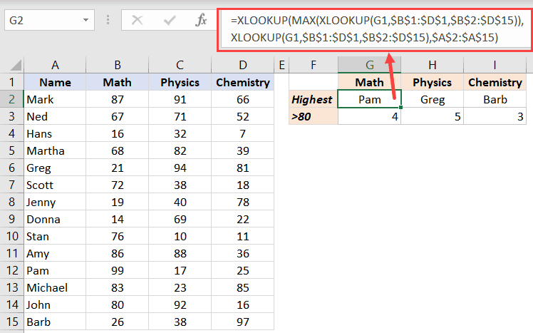
This one simply uses the XLOOKUP formula to get a range of all the values for the given subject. It then wraps it in COUNTIF function to get the number of scores that are more than 80.
Example 10: Using Wildcard in XLOOKUP
Just like you can use wildcard characters in VLOOKUP and MATCH, you can also do this with XLOOKUP.
But there is a difference.
In XLOOKUP, you need to specify that you’re using wildcard characters (in the fifth argument). If you don’t specify this, XLOOKUP will give you an error.
Below is a dataset where I have company names and their market capitalization.

I want to look up a company name in column D, and fetch the market capitalization from the table on the left. And since the names in Column D are not exact matches, I will have to use wildcard characters.
Below is the formula that will do this:
=XLOOKUP("*"&D2&"*",$A$2:$A$11,$B$2:$B$11,,2)

In the above formula, I have used asterisk (*) wildcard character before as after D2 (it needs to be within double quotes and joined with D2 using ampersand).
This tells the formula to look through all the cells, and if it contains the word in cell D2 (which is Apple), consider it an exact match. No matter how many and what characters are before and after the text in cell D2.
And to make sure XLOOKUP accepts wildcard characters, the fifth argument has been set to 2 (wildcard character match).
Example 11: Find the Last Value in the Column
Since XLOOKUP allows you to search from bottom to top, you can easily find the last value in a list, as well as fetch the corresponding value from a column.
Suppose you have a dataset as shown below and you want to know what’s the last company and what’s the market capitalization of this last company.

The below formula will give you the name of the last company:
=XLOOKUP("*",A2:A11,A2:A11,,2,-1)
And the below formula will give the market cap of the last company in the list:
=XLOOKUP("*",A2:A11,B2:B11,,2,-1)

These formulas again use wildcard characters. In these, I have used asterisk (*) as the lookup value, which means that this would consider the first cell it encounters as an exact match (as asterisk could be any character and any number of characters).
And since the direction is from bottom to top (for the vertically arranged data), it will return the last value in the list.
And the second formula since uses a separate return_range to get the market cap of the last name in the list.
Click here to download the example file and follow along
What if You don’t have XLOOKUP?
Since XLOOKUP will likely only be available to Office 365 users, one way to get it is to upgrade to Office 365.
If you already have Office 365 Home, Personal, or University edition, you already have access to XLOOKUP. All you need to do is join the Office Insider program.
To do this, go to the File tab, click on Account and then click on the Office insider option. There would be an option to join the insider program.
In case you have other Office 365 subscriptions (such as Enterprise), I am sure XLOOKUP and other awesome features (such as dynamic arrays, formulas such as SORT and FILTER) would become available soon.
In case you’re using Excel 2010/2013/2016/2019, you won’t have XLOOKUP, and you will have to continue to use VLOOKUP, HLOOKUP, and INDEX/MATCH combo to get the best out of lookup formulas.
XLOOKUP Backward Compatibility
This is one thing you need to be careful about – XLOOKUP is NOT backward compatible.
This means that if you create a file and use the XLOOKUP formula, and then open it in a version that doesn’t have XLOOKUP, it will show errors.
Since XLOOKUP is a huge step forward in the right direction, I believe this will become the default lookup formula, but it will surely take a few years before getting widely adopted. After all, I still see some people using Excel 2003.
So these are 11 XLOOKUP Examples that can help you do all the lookup and reference stuff done faster and also make it easy to use.
Hope you found this tutorial useful!
You may also like the following Excel tutorials:
- How to Compare Two Excel Sheets (for differences)
- How to Compare Two Columns in Excel (for matches & differences)
- Find the Last Occurrence of a Lookup Value a List in Excel
- Lookup the Second, the Third, or the Nth Value in Excel
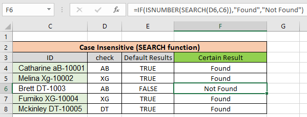
In this article, we will learn How to look up cells having certain text and return the Certain Text in Excel.
Scenario :
Identify particular text in a cell or different word in given cells. For example finding the department ID from a database. I think you must have thought to do it manually but time constraint. You are here at the right place to learn How to check if a cell contains specific text.
Generic formula:
The text you are looking for can either be exact or case insensitive. Case insensitive means formula looks for AG can return ag, Ag, AG or aG.
Case insensitive formula:
=ISNUMBER(SEARCH(find_text,within_text)
find_text : text to find
within_text : to find in text
Case sensitive formula:
=ISNUMBER(FIND(find_text,within_text)
find_text : text to find
within_text : to find in text
Note:
The above formulas will return True or False. Use the IF function with formula to return YES or NO. Use the below formula to get the certain required result format.
Case insensitive formula:
=IF(ISNUMBER(SEARCH(find_text,within_text)),»value_if_true»,value_if_false)
find_text : text to find
within_text : to find in text
Case sensitive formula:
=IF(ISNUMBER(FIND(find_text,within_text)),»value_if_true»,value_if_false)
find_text : text to find
within_text : to find in text
Note: In The above mentioned formula you can input values like YES/NO or Found/Notfound.
Example :
All of these might be confusing to understand. Let’s understand how to use the function using an example. Here we have some employees to look up by the given department Id. Employee id has name, department id and particular id. Here lookup text is in column D and within text is in Column C.
Use the formula:
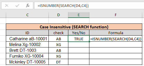
As you can see the formula finds AB when you looked for
AB using the Search function. Copy the formula to the rest of the cells using the Ctrl + D or dragging it down from the right bottom (tiny box) of the applied cell.
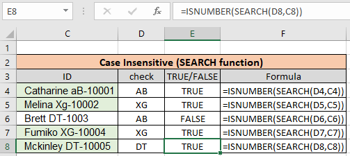
As you can see we found all the given department id employees using the above method. Now we will check if all cells contain specific text.
Another Example: (Case Sensitive)
Here we have been given a list of Employee Id information in column A and the look up department is «XG». Here we need to find the department «XG» in all cells. «XG» must be exact as there are two different departments that go by «Xg». So check only «XG» in all cells and return «Yes» if found and return «No» If not.
Use the formula:
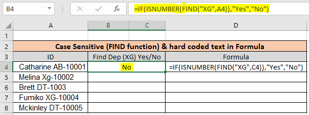
As you can see First employee doesn’t belong to «XG» so the formula returns «No» using the FIND function. Copy the formula to the rest of the cells using the Ctrl + D or dragging it down from the right bottom (tiny box) of the applied cell.
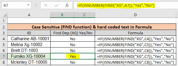
As you can see there is only one employee in «XG» department. This formula is useful wherever the database contains multiple information of a row in one cell.
Check if cell Matches multiple text
In the above example we lookup one given text in cells. If we have multiple texts then we use the SUMPRODUCT function, This formula returns TRUE/FALSE as per the value found/ Not found.
Use the formula:
=SUMPRODUCT(—ISNUMBER(SEARCH(,A1)))>0
Learn more about this formula. Follow this link How to Check if a string contains one of many texts in Excel.
Here are all the observational notes using the above explained formulas in Excel
Notes :
- Use the «find_text» in quotes when using hard coded values. Or else use cell reference as explained in the first example.
- SEARCH is case insensitive function whereas FIND is the case Sensitive dunction.
- Use the IF function, if you want to get the result in required forms like YES/NO or Found/Notfound.
Hope this article about How to lookup cells having certain text and returns the Certain Text in Excel is explanatory. Find more articles on calculating values and related Excel formulas here. If you liked our blogs, share it with your friends on Facebook. And also you can follow us on Twitter and Facebook. We would love to hear from you, do let us know how we can improve, complement or innovate our work and make it better for you. Write to us at info@exceltip.com.
Related Articles :
Searching a String for a Specific Substring in Excel : Find cells if cell contains given word in Excel using the FIND or SEARCH function.
Highlight cells that contain specific text : Highlight cells if cell contains given word in Excel using the formula under Conditional formatting
How to Check if a string contains one of many texts in Excel : lookup cells if cell contains from given multiple words in Excel using the FIND or SEARCH function.
Count Cells that contain specific text : Count number of cells if cell contains given text using one formula in Excel.
How to lookup cells having certain text and returns the Certain Text in Excel : find cells if cell contains certain text and returns required results using the IF function in Excel.
Popular Articles :
How to use the IF Function in Excel : The IF statement in Excel checks the condition and returns a specific value if the condition is TRUE or returns another specific value if FALSE.
How to use the VLOOKUP Function in Excel : This is one of the most used and popular functions of excel that is used to lookup value from different ranges and sheets.
How to use the SUMIF Function in Excel : This is another dashboard essential function. This helps you sum up values on specific conditions.
How to use the COUNTIF Function in Excel : Count values with conditions using this amazing function. You don’t need to filter your data to count specific values. Countif function is essential to prepare your dashboard.

Update: Based on questions I’ve received, I added the Misc Notes section to the end of this post.
Continuing with our #FunctionFriday series, today we’re going to explore how to use the IF, SEARCH, and ISNUMBER functions together to find text (aka a string) inside other text for classification purpose. What Excel really needs is a CONTAINS function, so we don’t have to do these mental acrobats. But, for now, this is what we have to work with.
To illustrate it, I’ll use an example from a chart I include in client dashboards** where they use the AddThis or ShareThis WordPress plugin. The data from these plugins populates to your Google Analytics account. BUT the data is such a red-hot mess, you have to do some cleanup to get it all into nice, neat buckets.
If you’d like to include this report in your own reports, you can use this custom report I created. (If you get a 404 error, it’s because you’re not logged in to Google Analytics. You have to be logged in to apply the report to your Google Analytics profile, aka view.)
**If you want to become a beast at building dashboards using the Google Analytics API, my online course will take you there.
Download Excel Workbook
If you’d like to follow along, you can download the Excel workbook I used in this demo.
The Functions du Jour
IF Function
The IF function is the Swiss Army knife for marketers, especially when you’re building out dynamic dashboards. With the IF function you start with a test — e.g., if A3=B2, if A3>=100, if A3=”organic”, etc. — and then you specify what you want to return if the condition is true and what you want to return if the value is false. But the fun doesn’t stop there; you can actually embed IF functions inside of IF functions. And that’s what we’re going to do in this tutorial.
It follows the following syntax:
IF(logical_test, [value_if_true], [value_if_false])
SEARCH Function
The SEARCH function is a tricky little bugger. It returns the position of whatever character you search for. And if you enter a string of characters, it will return the position of the first character in the matching string. So if you searched for cheese in the string string cheese, it would return the value of 8.
The SEARCH function follows the following syntax:
SEARCH( substring, string, [start_position] )
substring: Pure, unbridled geek speak that means whatever text you’re searching for, e.g., cheese.
string: Typically the cell this text string is in, though you could enter text as long as you flank it with quotation marks. (I almost always use a cell reference.)
start_position: This is optional. I usually only use it when I’m searching for forward slashes in URLs and want to start searching after the http(s)://. You can check out an example in this post that describes how to extract domains from URLs.
Now, if you put a string inside a SEARCH function, it will look for that string exactly. But you can also throw the asterisk wildcard in there for a really good time, which tells Excel to flag any string that even contains the text you’re searching for. So going back to our string cheese example, if I searched for cheese, it would return FALSE; if I searched for *cheese*, it would return TRUE.
ISNUMBER Function
The ISNUMBER function simply tells you if the cell you’re referencing is a value (or number). It’s Boolean, meaning it returns either a value of TRUE or FALSE.
It follows the following syntax:
ISNUMBER(value)
Pro Tip
When dealing with a more complicated IF function, like you’ll see below, a good strategy is to break it into separate lines in the formula bar. To add a line break on a PC, use Alt-Enter; on a Mac, use Control-Option-Enter. I break my IF functions into different lines if I have more than three nested IFs. Here’s what it looks like for the formula we’ll use:
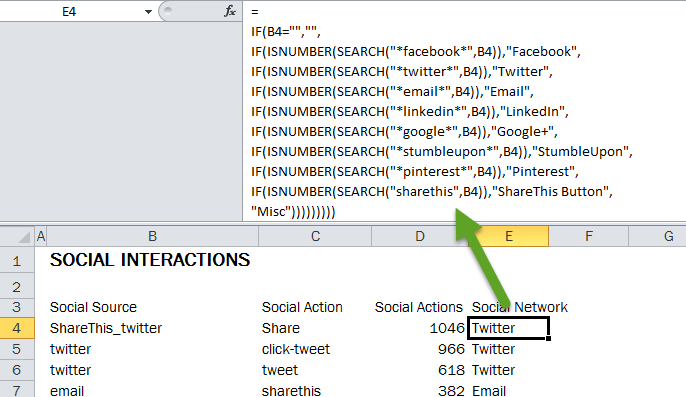
If you fat finger something in your formula, it’s really easy to see using this strategy because the IF functions won’t line up. When I’m finished, I just collapse the formula bar back to size by clicking-and-dragging the bottom of it.
Here’s what that same formula would look like if I didn’t use line breaks:

Putting It All Together
Okay, so here’s how we’re going to use them in concert. The Google Analytics custom report we’re using in this demo uses two dimensions: Social Source and Social Action and one metric, Social Actions. It’s a flat report, which, betedubs, is perfect for pivot tables. (Again, you should have data in this report if you use the ShareThis or AddThis plugin on WordPress.) But you could use this same strategy with any marketing data that you have to bucket based on snippets of text inside of strings.
If the formula in cell E4 could talk in plain English (wouldn’t that be nice?), here’s what it would say: “Hey, Excel, check out cell B4. If you see the string facebook anywhere in there, ISNUMBER will return a value of TRUE because you’ll return a number telling me the position of where the string I’m searching for. I don’t actually care about where that string is, only that it returns a number. If it does (IOW, it returns a value of TRUE), return the string Facebook; if it’s false, look for the next sting (i.e., twitter) and return Twitter … Rinse and repeat until you’ve cycled through all of the criteria. And if you don’t find facebook, twitter, email, linkedin, google, stumbleupon, pinterest, or sharethis, just call it Misc.” (Obviously, switch out sharethis for addthis if you’re using that plugin.)
Misc Notes
Difference Between SEARCH and FIND
Someone asked me about using the FIND function on Facebook instead of SEARCH. I rarely use the FIND function because it’s not as flexible as SEARCH. For one, it’s case sensitive. I can only remember one time using it because I needed to differentiate between cases. A much bigger liability is you can’t use it for partial matches because it doesn’t support Excel’s wildcard characters (* and ?).
Extracting Text Instead Of Categorizing It
So what if you didn’t want to match exact or partial text for the purpose of categorizing it like I have in this post with the help of the IF and ISNUMBER functions? What if, instead, you wanted to extract it instead? Then you would use the SEARCH function with the LEFT, RIGHT, and/or MID functions. I demonstrate how to do that in this tutorial on pulling domain names from a list of URLs. (I use this technique in conjunction with pivot tables in just about all competitive analysis I do because it allows me to group backlinks by domain.)
Image credit
~~~
If you would like to learn more about Excel, check out my Excel dashboard course. 24 instructional videos, totaling 6+ hours of instruction for $95.