
17 авг. 2022 г.
читать 3 мин
Логистическая регрессия — это метод, который мы используем для подбора регрессионной модели, когда переменная ответа является бинарной.
В этом руководстве объясняется, как выполнить логистическую регрессию в Excel.
Пример: логистическая регрессия в Excel
Используйте следующие шаги, чтобы выполнить логистическую регрессию в Excel для набора данных, который показывает, были ли баскетболисты колледжей выбраны в НБА (драфт: 0 = нет, 1 = да) на основе их среднего количества очков, подборов и передач в предыдущем время года.
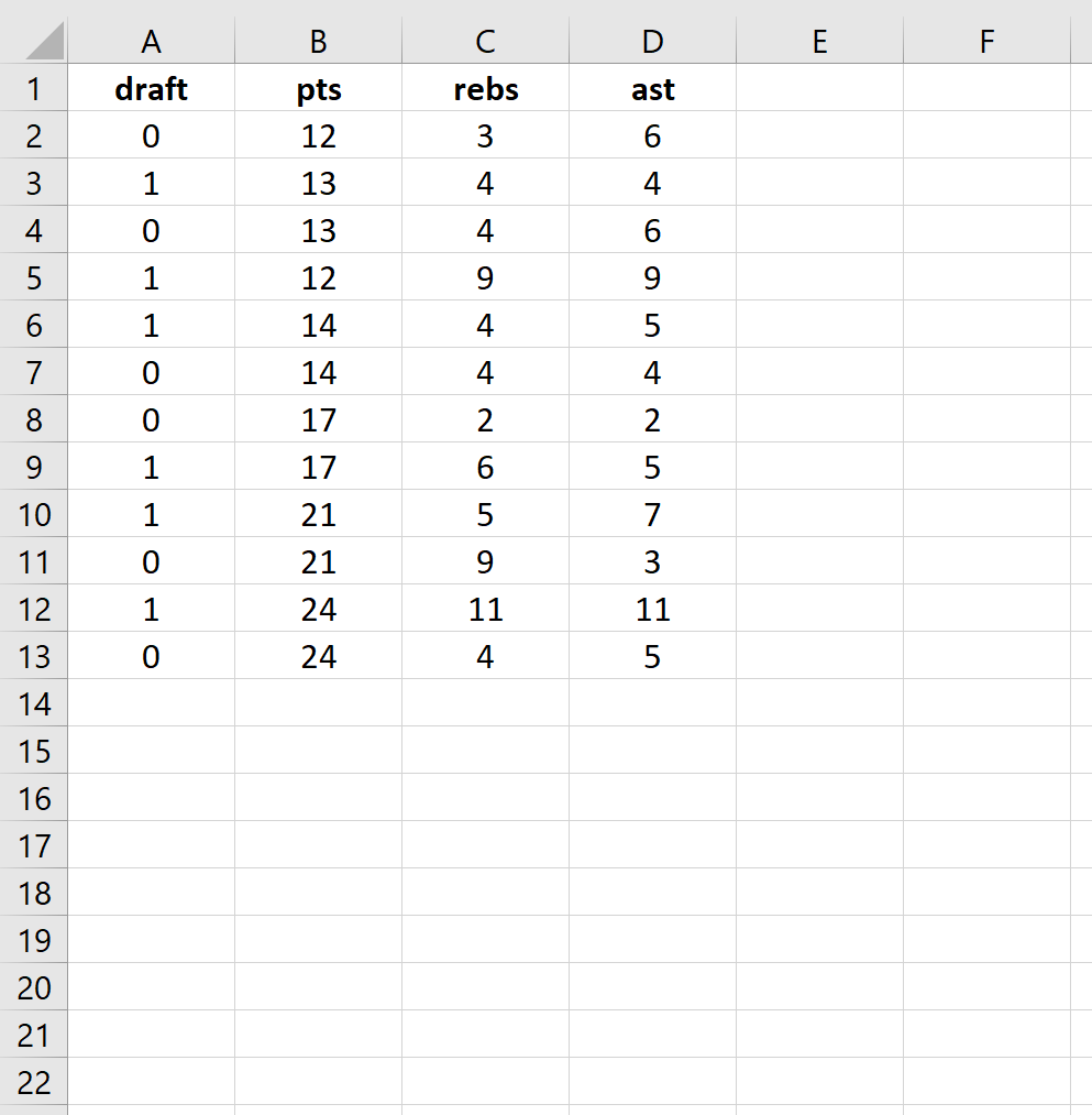
Шаг 1: Введите данные.
Сначала введите следующие данные:
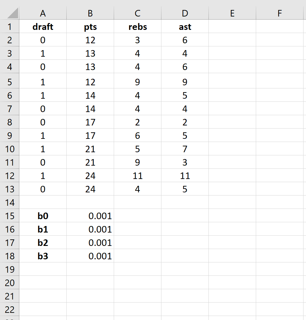
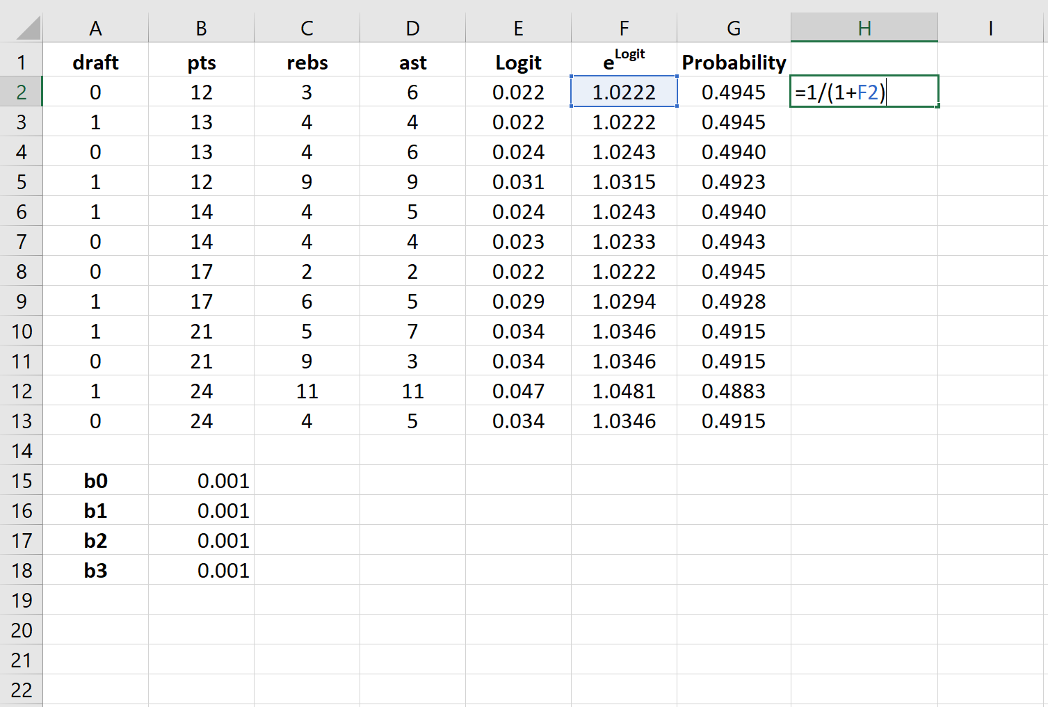
Шаг 2: Введите ячейки для коэффициентов регрессии.
Поскольку в модели у нас есть три объясняющие переменные (pts, rebs, ast), мы создадим ячейки для трех коэффициентов регрессии плюс один для точки пересечения в модели. Мы установим значения для каждого из них на 0,001, но мы оптимизируем их позже.
Далее нам нужно будет создать несколько новых столбцов, которые мы будем использовать для оптимизации этих коэффициентов регрессии, включая логит, e логит , вероятность и логарифмическую вероятность.
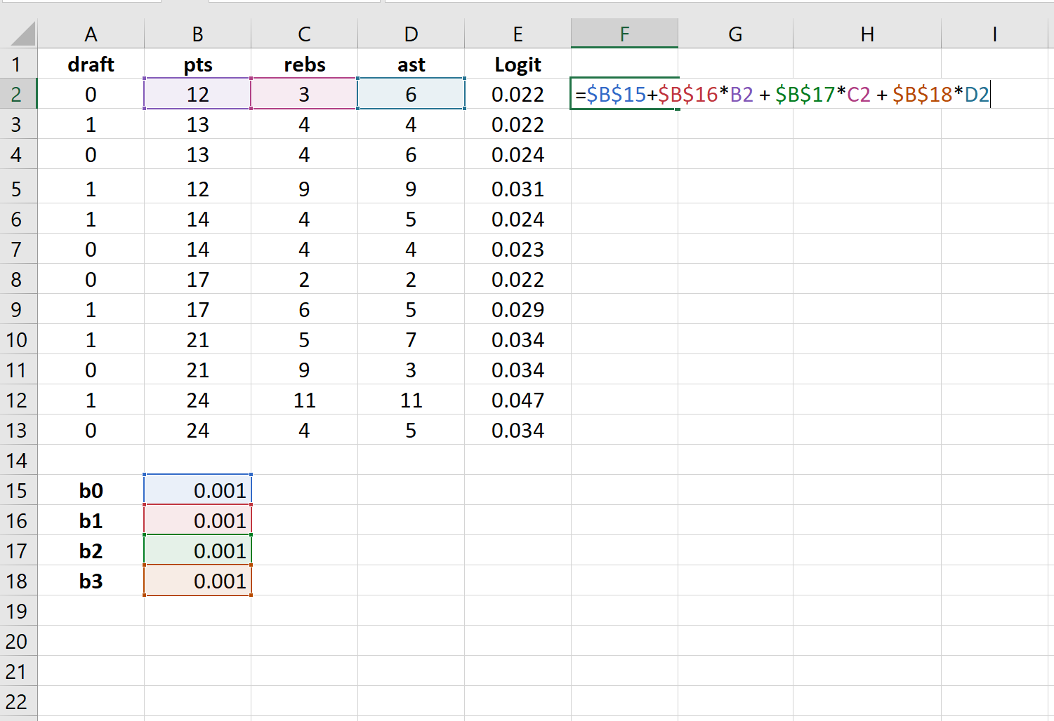
Шаг 3: Создайте значения для логита.
Далее мы создадим столбец logit, используя следующую формулу:
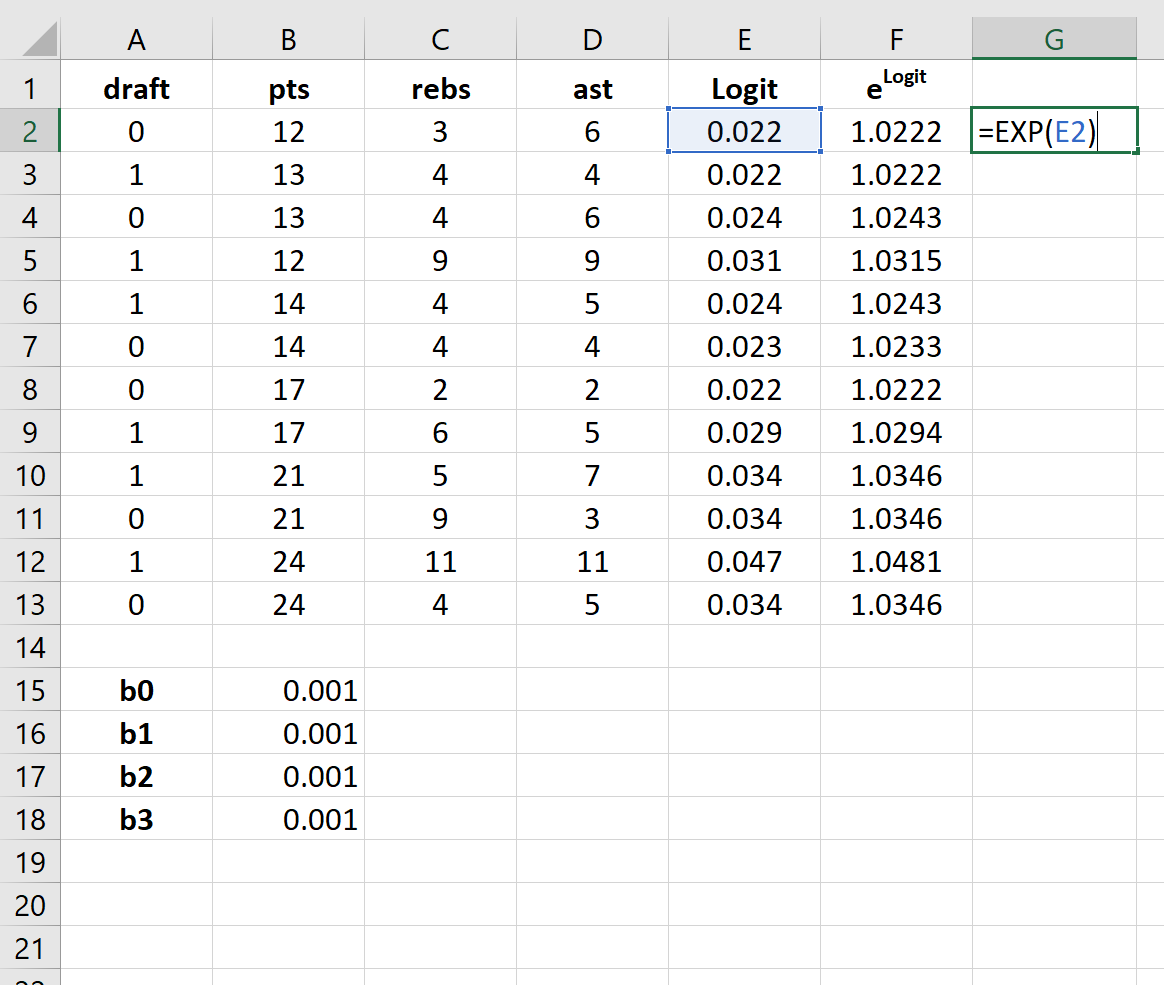
Шаг 4: Создайте значения для e logit .
Далее мы создадим значения для e logit , используя следующую формулу:
Шаг 5: Создайте значения для вероятности.
Далее мы создадим значения вероятности, используя следующую формулу:
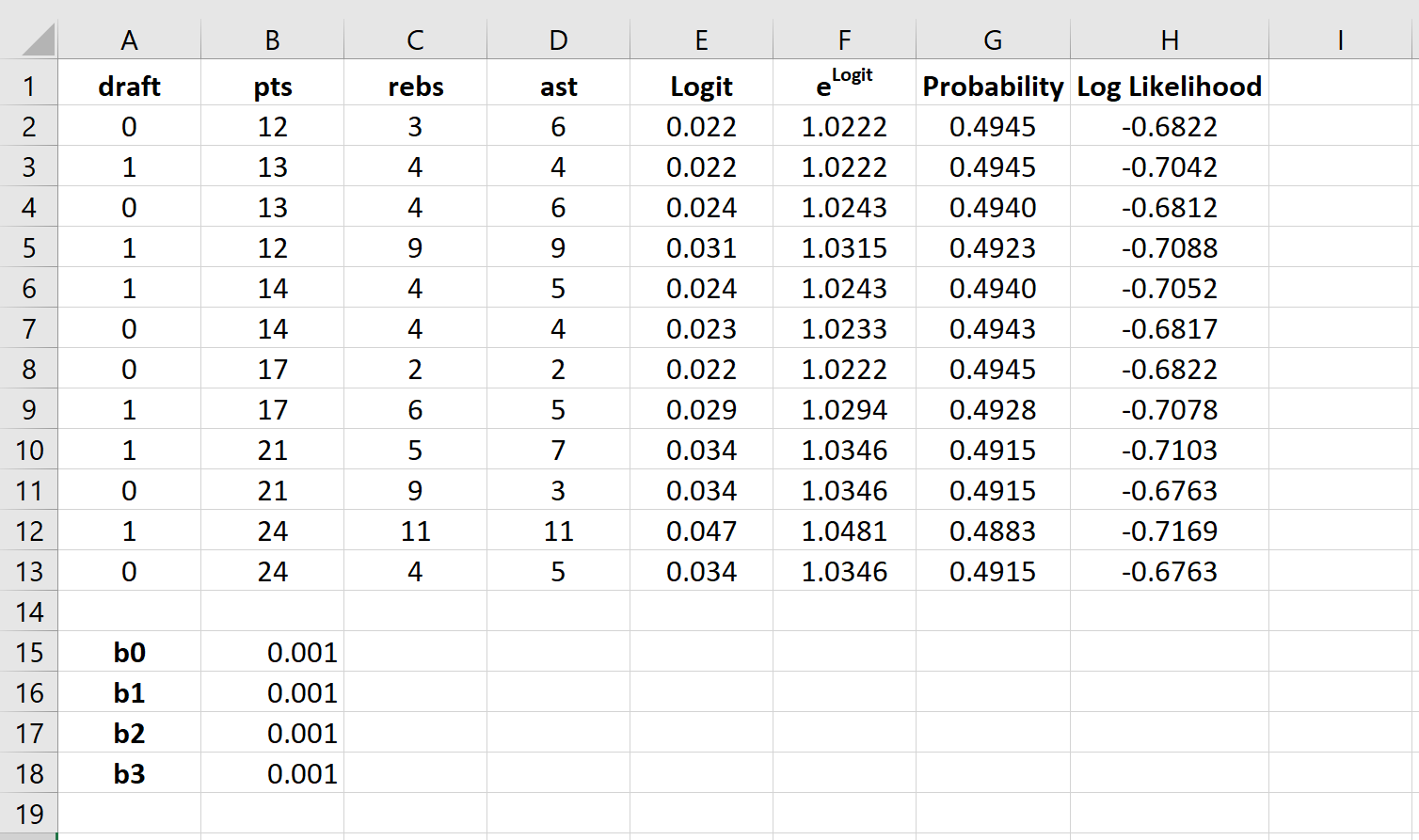
Шаг 6: Создайте значения для логарифмической вероятности.
Далее мы создадим значения для логарифмической вероятности, используя следующую формулу:
Логарифмическая вероятность = LN (вероятность)
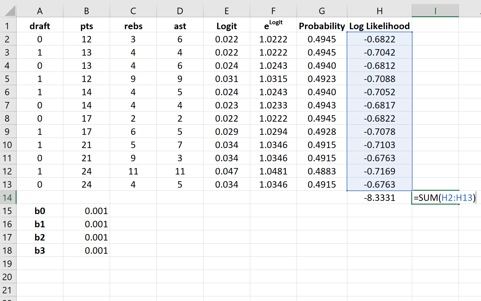
Шаг 7: Найдите сумму логарифмических вероятностей.
Наконец, мы найдем сумму логарифмических правдоподобий, то есть число, которое мы попытаемся максимизировать, чтобы найти коэффициенты регрессии.
Шаг 8: Используйте Решатель, чтобы найти коэффициенты регрессии.
Если вы еще не установили Solver в Excel, выполните следующие действия:
- Щелкните Файл .
- Щелкните Параметры .
- Щелкните Надстройки .
- Нажмите Надстройка «Поиск решения» , затем нажмите «Перейти» .
- В новом всплывающем окне установите флажок рядом с Solver Add-In , затем нажмите «Перейти» .
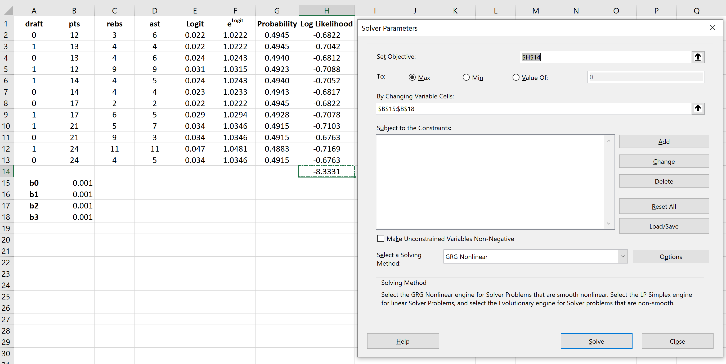
После установки Солвера перейдите в группу Анализ на вкладке Данные и нажмите Солвер.Введите следующую информацию:
- Установите цель: выберите ячейку H14, содержащую сумму логарифмических вероятностей.
- Путем изменения ячеек переменных: выберите диапазон ячеек B15:B18, который содержит коэффициенты регрессии.
- Сделать неограниченные переменные неотрицательными: снимите этот флажок.
- Выберите метод решения: выберите GRG Nonlinear.
Затем нажмите «Решить» .
Решатель автоматически вычисляет оценки коэффициента регрессии:
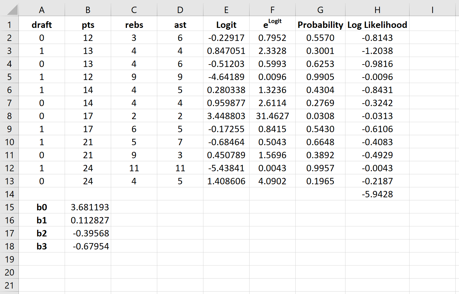
По умолчанию коэффициенты регрессии можно использовать для определения вероятности того, что осадка = 0. Однако обычно в логистической регрессии нас интересует вероятность того, что переменная отклика = 1. Таким образом, мы можем просто поменять знаки на каждом из коэффициенты регрессии:
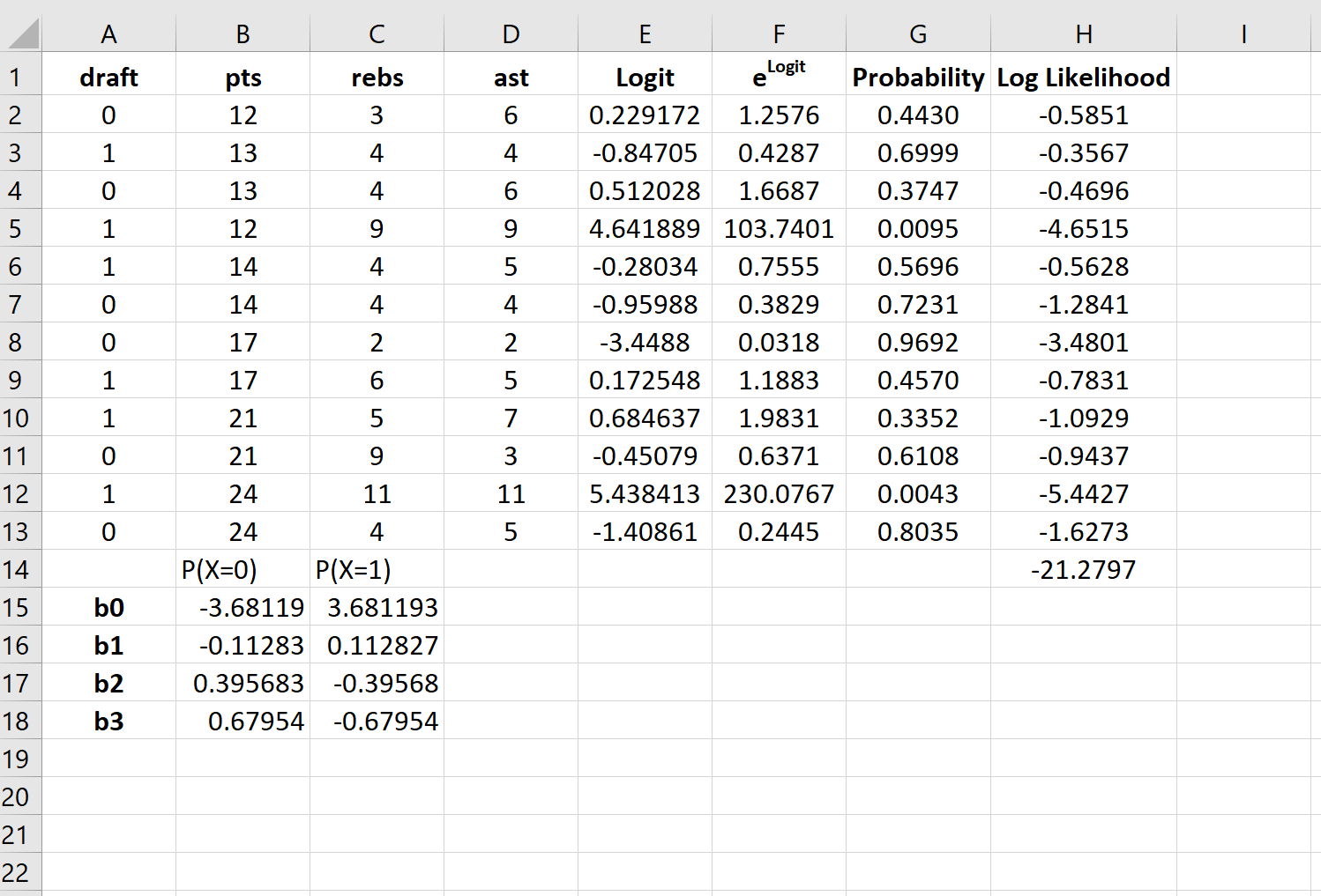
Теперь эти коэффициенты регрессии можно использовать для определения вероятности того, что осадка = 1.
Например, предположим, что игрок набирает в среднем 14 очков за игру, 4 подбора за игру и 5 передач за игру. Вероятность того, что этот игрок будет выбран в НБА, можно рассчитать как:
P(draft = 1) = e 3,681193 + 0,112827*(14) -0,39568*(4) – 0,67954*(5) / (1+e 3,681193 + 0,112827*(14) -0,39568*(4) – 0,67954*(5) ) ) = 0,57 .
Поскольку эта вероятность больше 0,5, мы прогнозируем, что этот игрокпопасть в НБА.
Связанный: Как создать кривую ROC в Excel (шаг за шагом)
Logistic regression is a method that we use to fit a regression model when the response variable is binary.
This tutorial explains how to perform logistic regression in Excel.
Example: Logistic Regression in Excel
Use the following steps to perform logistic regression in Excel for a dataset that shows whether or not college basketball players got drafted into the NBA (draft: 0 = no, 1 = yes) based on their average points, rebounds, and assists in the previous season.
Step 1: Input the data.
First, input the following data:

Step 2: Enter cells for regression coefficients.
Since we have three explanatory variables in the model (pts, rebs, ast), we will create cells for three regression coefficients plus one for the intercept in the model. We will set the values for each of these to 0.001, but we will optimize for them later.

Next, we will have to create a few new columns that we will use to optimize for these regression coefficients including the logit, elogit, probability, and log likelihood.
Step 3: Create values for the logit.
Next, we will create the logit column by using the the following formula:

Step 4: Create values for elogit.
Next, we will create values for elogit by using the following formula:

Step 5: Create values for probability.
Next, we will create values for probability by using the following formula:

Step 6: Create values for log likelihood.
Next, we will create values for log likelihood by using the following formula:
Log likelihood = LN(Probability)

Step 7: Find the sum of the log likelihoods.
Lastly, we will find the sum of the log likelihoods, which is the number we will attempt to maximize to solve for the regression coefficients.

Step 8: Use the Solver to solve for the regression coefficients.
If you haven’t already install the Solver in Excel, use the following steps to do so:
- Click File.
- Click Options.
- Click Add-Ins.
- Click Solver Add-In, then click Go.
- In the new window that pops up, check the box next to Solver Add-In, then click Go.
Once the Solver is installed, go to the Analysis group on the Data tab and click Solver. Enter the following information:
- Set Objective: Choose cell H14 that contains the sum of the log likelihoods.
- By Changing Variable Cells: Choose the cell range B15:B18 that contains the regression coefficients.
- Make Unconstrained Variables Non-Negative: Uncheck this box.
- Select a Solving Method: Choose GRG Nonlinear.
Then click Solve.
The Solver automatically calculates the regression coefficient estimates:

By default, the regression coefficients can be used to find the probability that draft = 0.
However, typically in logistic regression we’re interested in the probability that the response variable = 1.
So, we can simply reverse the signs on each of the regression coefficients:

Now these regression coefficients can be used to find the probability that draft = 1.
For example, suppose a player averages 14 points per game, 4 rebounds per game, and 5 assists per game. The probability that this player will get drafted into the NBA can be calculated as:
P(draft = 1) = e3.681193 + 0.112827*(14) -0.39568*(4) – 0.67954*(5) / (1+e3.681193 + 0.112827*(14) -0.39568*(4) – 0.67954*(5)) = 0.57.
Since this probability is greater than 0.5, we predict that this player would get drafted into the NBA.
Related: How to Create a ROC Curve in Excel (Step-by-Step)
Содержание
- Как выполнить логистическую регрессию в Excel
- Пример: логистическая регрессия в Excel
- How to Perform Logistic Regression in Excel
- Example: Logistic Regression in Excel
- Do logistic regression excel
Как выполнить логистическую регрессию в Excel

Логистическая регрессия — это метод, который мы используем для подбора регрессионной модели, когда переменная ответа является бинарной.
В этом руководстве объясняется, как выполнить логистическую регрессию в Excel.
Пример: логистическая регрессия в Excel
Используйте следующие шаги, чтобы выполнить логистическую регрессию в Excel для набора данных, который показывает, были ли баскетболисты колледжей выбраны в НБА (драфт: 0 = нет, 1 = да) на основе их среднего количества очков, подборов и передач в предыдущем время года.
Шаг 1: Введите данные.
Сначала введите следующие данные:
Шаг 2: Введите ячейки для коэффициентов регрессии.
Поскольку в модели у нас есть три объясняющие переменные (pts, rebs, ast), мы создадим ячейки для трех коэффициентов регрессии плюс один для точки пересечения в модели. Мы установим значения для каждого из них на 0,001, но мы оптимизируем их позже.
Далее нам нужно будет создать несколько новых столбцов, которые мы будем использовать для оптимизации этих коэффициентов регрессии, включая логит, e логит , вероятность и логарифмическую вероятность.
Шаг 3: Создайте значения для логита.
Далее мы создадим столбец logit, используя следующую формулу:
Шаг 4: Создайте значения для e logit .
Далее мы создадим значения для e logit , используя следующую формулу:
Шаг 5: Создайте значения для вероятности.
Далее мы создадим значения вероятности, используя следующую формулу:
Шаг 6: Создайте значения для логарифмической вероятности.
Далее мы создадим значения для логарифмической вероятности, используя следующую формулу:
Логарифмическая вероятность = LN (вероятность)
Шаг 7: Найдите сумму логарифмических вероятностей.
Наконец, мы найдем сумму логарифмических правдоподобий, то есть число, которое мы попытаемся максимизировать, чтобы найти коэффициенты регрессии.
Шаг 8: Используйте Решатель, чтобы найти коэффициенты регрессии.
Если вы еще не установили Solver в Excel, выполните следующие действия:
- Щелкните Файл .
- Щелкните Параметры .
- Щелкните Надстройки .
- Нажмите Надстройка «Поиск решения» , затем нажмите «Перейти» .
- В новом всплывающем окне установите флажок рядом с Solver Add-In , затем нажмите «Перейти» .
После установки Солвера перейдите в группу Анализ на вкладке Данные и нажмите Солвер.Введите следующую информацию:
- Установите цель: выберите ячейку H14, содержащую сумму логарифмических вероятностей.
- Путем изменения ячеек переменных: выберите диапазон ячеек B15:B18, который содержит коэффициенты регрессии.
- Сделать неограниченные переменные неотрицательными: снимите этот флажок.
- Выберите метод решения: выберите GRG Nonlinear.
Затем нажмите «Решить» .
Решатель автоматически вычисляет оценки коэффициента регрессии:
По умолчанию коэффициенты регрессии можно использовать для определения вероятности того, что осадка = 0. Однако обычно в логистической регрессии нас интересует вероятность того, что переменная отклика = 1. Таким образом, мы можем просто поменять знаки на каждом из коэффициенты регрессии:
Теперь эти коэффициенты регрессии можно использовать для определения вероятности того, что осадка = 1.
Например, предположим, что игрок набирает в среднем 14 очков за игру, 4 подбора за игру и 5 передач за игру. Вероятность того, что этот игрок будет выбран в НБА, можно рассчитать как:
P(draft = 1) = e 3,681193 + 0,112827*(14) -0,39568*(4) – 0,67954*(5) / (1+e 3,681193 + 0,112827*(14) -0,39568*(4) – 0,67954*(5) ) ) = 0,57 .
Поскольку эта вероятность больше 0,5, мы прогнозируем, что этот игрокпопасть в НБА.
Источник
How to Perform Logistic Regression in Excel
Logistic regression is a method that we use to fit a regression model when the response variable is binary.
This tutorial explains how to perform logistic regression in Excel.
Example: Logistic Regression in Excel
Use the following steps to perform logistic regression in Excel for a dataset that shows whether or not college basketball players got drafted into the NBA (draft: 0 = no, 1 = yes) based on their average points, rebounds, and assists in the previous season.
Step 1: Input the data.
First, input the following data:
Step 2: Enter cells for regression coefficients.
Since we have three explanatory variables in the model (pts, rebs, ast), we will create cells for three regression coefficients plus one for the intercept in the model. We will set the values for each of these to 0.001, but we will optimize for them later.
Next, we will have to create a few new columns that we will use to optimize for these regression coefficients including the logit, e logit , probability, and log likelihood.
Step 3: Create values for the logit.
Next, we will create the logit column by using the the following formula:
Step 4: Create values for e logit .
Next, we will create values for e logit by using the following formula:
Step 5: Create values for probability.
Next, we will create values for probability by using the following formula:
Step 6: Create values for log likelihood.
Next, we will create values for log likelihood by using the following formula:
Log likelihood = LN(Probability)
Step 7: Find the sum of the log likelihoods.
Lastly, we will find the sum of the log likelihoods, which is the number we will attempt to maximize to solve for the regression coefficients.
Step 8: Use the Solver to solve for the regression coefficients.
If you haven’t already install the Solver in Excel, use the following steps to do so:
- Click File.
- Click Options.
- Click Add-Ins.
- Click Solver Add-In, then click Go.
- In the new window that pops up, check the box next to Solver Add-In, then click Go.
Once the Solver is installed, go to the Analysis group on the Data tab and click Solver. Enter the following information:
- Set Objective: Choose cell H14 that contains the sum of the log likelihoods.
- By Changing Variable Cells: Choose the cell range B15:B18 that contains the regression coefficients.
- Make Unconstrained Variables Non-Negative: Uncheck this box.
- Select a Solving Method: Choose GRG Nonlinear.
Then click Solve.
The Solver automatically calculates the regression coefficient estimates:
By default, the regression coefficients can be used to find the probability that draft = 0.
However, typically in logistic regression we’re interested in the probability that the response variable = 1.
So, we can simply reverse the signs on each of the regression coefficients:
Now these regression coefficients can be used to find the probability that draft = 1.
For example, suppose a player averages 14 points per game, 4 rebounds per game, and 5 assists per game. The probability that this player will get drafted into the NBA can be calculated as:
P(draft = 1) = e 3.681193 + 0.112827*(14) -0.39568*(4) – 0.67954*(5) / (1+e 3.681193 + 0.112827*(14) -0.39568*(4) – 0.67954*(5) ) = 0.57.
Since this probability is greater than 0.5, we predict that this player would get drafted into the NBA.
Источник
Do logistic regression excel
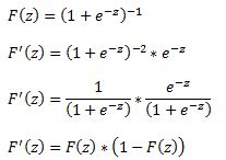
A logit model is a type of a binary choice model. We use a logistic equation to assign a probability to an event. We define a logistic cumulative density function as:

which is equivalent to


Another property of the logistic function is that:

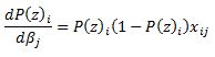
The first derivative of the logistic function, which we will need when deriving the coefficients of our model, with respect to z is:

In a logistic regression model we set up the equation below:

In this set up using ordinary least squares to estimate the beta coefficients is impossible so we must rely on maximum likelihood method.
Under the assumption that each observation of the dependent variable is random and independent we can derive a likelihood function. The likelihood that we observe our existing sample under the assumption of independence is simply the product of the probability of each observation.
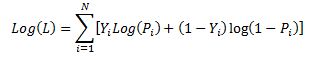
Our likelihood function is:

Where Y is either 0 or 1. We can see that when Y =1 then we have P and when Y=0 we have (1-P)
The aim of the maximum likelihood method is to derive the coefficients of the model that maximize the likelihood function. It is much easier to work with the log of the likelihood function.

From calculus we know that a functions maximum is at a point where its first derivative is equal to zero. Therefore our approach is to take the derivative of the log likelihood function with respect to each beta and derive the value of betas for which the first derivative is equal to zero. This cannot be done analytically unfortunately so we must resolve to using a numerical method. Fortunately for us the log likelihood function has nice properties that allows us to use Newton’s method to achieve this.
Newton’s method is easiest to understand in a univariate set up. It is a numerical method for finding a root of a function by successively making better approximations to the root based on the functions gradient (first derivative).
As a quick example we know that we can approximate a function using first order Taylor series approximation.

where Xc is the current estimate of the root. By setting the function to zero we get

This means that in each step of the algorithm we can improve on an initial guess for x using above rule. Same principles apply to a multivariate system of equations:

Here x is a vector of x values and J is the Jacobian matrix of first derivatives evaluated at vector xc and F is the value of the function evaluated at using latest estimates of x.
Coming back to our logistic regression problem what we are trying to do is to figure out a combination of beta parameters for which our log likelihood function is at a maximum which is equivalent to deriving the set of coefficients where the first derivatives of the likelihood function are all equal to zero. We will do this by using Newton’s numerical method. In the notation from above F is the collection of our log likelihood function’s derivatives with respect to each beta and J is the Hessian matrix of second order partial derivatives of the likelihood function with respect to each beta.
It is a little tedious but necessary to work out these derivatives analytically so we can feed them into our spreadsheet.
Lets restate the log likelihood function once more:

And lets remember that in our case Pi is modeled as:

We will list all the steps in the calculations for those who wish to double check the work
First lets calculate

and via chain rule


and via chain rule

Now we can work through the derivative of our likelihood function.

The derivative of Y with respect to beta (highlighted in red) is equal to zero so we are left with:

Now we can substitute our calculated derivatives:

Values in red cancel out and we are left with:

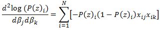
Now we need to calculate the Hessian matrix. Remembering that:


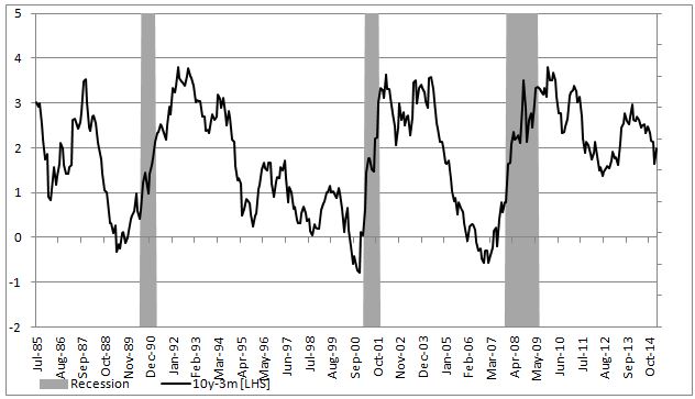
To show an example of how to implement this in excel we will attempt to model the probability of a recession in US (as defined by NBER) with a 3 month lead time. In our set up Y = 1 if US experiences a recession in 3months time and 0 otherwise. Our explanatory variable will be the 10yr3mth treasury curve spread. The yield curve is widely considered to be a leading indicator for economic slowdowns and curve inversion is often considered a sign of a recession.
In the chart below we highlight US recessions in grey while the black line is the yield curve.
The model we are trying to estimate is:

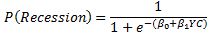
In a spreadsheet we load data on historical recessions in column C and our dependent variable in column D which refers to column C but 3 months ahead. In column E we input 1 which will be our intercept. Column F has historical values for the yield curve. In column G we calculate the probability with the above formula. Our initial guess for betas is zero which we have entered in cell C2 and C3.

In column H we calculate the log likelihood function for each observation. we sum all the values in cell H5. Therefore H5 contains the value of the below formula while each row has a value for each i in the brackets.

Column I calculates the derivative of the likelihood function for each observation with respect to the intercept. Column J calculates the derivative of the likelihood function for each observation with respect to the second beta. The sum of the totals for each column are in cells I2 and I3.

Now we need to calculate the second order derivatives of the likelihood function with respect to each beta. We need 4 in total but remembering that (hessian matrix is symmetric) we only need to calculate 3 columns.

Column K through M calculates the partial derivatives for each row and the sums are reported in a matrix in range J2:K3

Now we finally need to calculate the incremental adjustment to our beta estimates as dictated by the Newton algorithm.

We can use Excel’s functions MINVERSE to calculate the inverse of the Hessian matrix and MMULT function to multiply by our Jacobian matrix. Inputting =MMULT(MINVERSE(J2:K3),I2:I3) in range H2:H3 and pressing Ctrl+Shift+Enter since these are array functions we get the marginal adjustment needed.
Finally in G2 we calculate the adjusted intercept beta by subtracting H2 from C2. We do the same for the second beta.

All the calculations shown so far constitute just one iteration of the Newton algorithm. The results so far look like below:

we can copy and paste as values range G2:G3 to C2:C3 to calculate the second iteration of the algorithm

Notice that the log likelihood function has increased. We now have our new estimates in G2:G3. We can copy and paste as values into C2:C3 again. And we should repeat this until the Jacobian matrix is showing zeroes. Once both entries in I2:I3 are zero our log likelihood function is at a maximum.
The algorithm has converged after only 6 iterations and we get below estimates for betas

Overall the model does a poor job of forecasting recessions. The red line shows the probabilities.

In a follow up post we will show how to implement logistic regression in VBA. We will also introduce statistical methods to validate the model and to check for statistical significance of the estimated parameters.
A final note, in this post we wanted to provide a thorough explanation of the logistic regression model and the empirical example we have chosen is too simplistic to be used in practice. However using this approach to model recession probabilities can be very fruitful. Below is an example of a six factor model using the same techniques that forecasts historical recession episodes very well.
Источник
A logit model is a type of a binary choice model. We use a logistic equation to assign a probability to an event. We define a logistic cumulative density function as:

which is equivalent to


Another property of the logistic function is that:

The first derivative of the logistic function, which we will need when deriving the coefficients of our model, with respect to z is:
In a logistic regression model we set up the equation below:

In this set up using ordinary least squares to estimate the beta coefficients is impossible so we must rely on maximum likelihood method.
Under the assumption that each observation of the dependent variable is random and independent we can derive a likelihood function. The likelihood that we observe our existing sample under the assumption of independence is simply the product of the probability of each observation.
Our likelihood function is:

Where Y is either 0 or 1. We can see that when Y =1 then we have P and when Y=0 we have (1-P)
The aim of the maximum likelihood method is to derive the coefficients of the model that maximize the likelihood function. It is much easier to work with the log of the likelihood function.
From calculus we know that a functions maximum is at a point where its first derivative is equal to zero. Therefore our approach is to take the derivative of the log likelihood function with respect to each beta and derive the value of betas for which the first derivative is equal to zero. This cannot be done analytically unfortunately so we must resolve to using a numerical method. Fortunately for us the log likelihood function has nice properties that allows us to use Newton’s method to achieve this.
Newton’s method is easiest to understand in a univariate set up. It is a numerical method for finding a root of a function by successively making better approximations to the root based on the functions gradient (first derivative).
As a quick example we know that we can approximate a function using first order Taylor series approximation.

where Xc is the current estimate of the root. By setting the function to zero we get

This means that in each step of the algorithm we can improve on an initial guess for x using above rule. Same principles apply to a multivariate system of equations:

Here x is a vector of x values and J is the Jacobian matrix of first derivatives evaluated at vector xc and F is the value of the function evaluated at using latest estimates of x.
Coming back to our logistic regression problem what we are trying to do is to figure out a combination of beta parameters for which our log likelihood function is at a maximum which is equivalent to deriving the set of coefficients where the first derivatives of the likelihood function are all equal to zero. We will do this by using Newton’s numerical method. In the notation from above F is the collection of our log likelihood function’s derivatives with respect to each beta and J is the Hessian matrix of second order partial derivatives of the likelihood function with respect to each beta.
It is a little tedious but necessary to work out these derivatives analytically so we can feed them into our spreadsheet.
Lets restate the log likelihood function once more:
And lets remember that in our case Pi is modeled as:

We will list all the steps in the calculations for those who wish to double check the work
First lets calculate

and via chain rule

Therefore

Also,

and via chain rule

Now we can work through the derivative of our likelihood function.

The derivative of Y with respect to beta (highlighted in red) is equal to zero so we are left with:

Now we can substitute our calculated derivatives:

Values in red cancel out and we are left with:

Now we need to calculate the Hessian matrix. Remembering that:
we have:
To show an example of how to implement this in excel we will attempt to model the probability of a recession in US (as defined by NBER) with a 3 month lead time. In our set up Y = 1 if US experiences a recession in 3months time and 0 otherwise. Our explanatory variable will be the 10yr3mth treasury curve spread. The yield curve is widely considered to be a leading indicator for economic slowdowns and curve inversion is often considered a sign of a recession.
In the chart below we highlight US recessions in grey while the black line is the yield curve.

The model we are trying to estimate is:
In a spreadsheet we load data on historical recessions in column C and our dependent variable in column D which refers to column C but 3 months ahead. In column E we input 1 which will be our intercept. Column F has historical values for the yield curve. In column G we calculate the probability with the above formula. Our initial guess for betas is zero which we have entered in cell C2 and C3.

In column H we calculate the log likelihood function for each observation. we sum all the values in cell H5. Therefore H5 contains the value of the below formula while each row has a value for each i in the brackets.

Column I calculates the derivative of the likelihood function for each observation with respect to the intercept. Column J calculates the derivative of the likelihood function for each observation with respect to the second beta. The sum of the totals for each column are in cells I2 and I3.

Now we need to calculate the second order derivatives of the likelihood function with respect to each beta. We need 4 in total but remembering that (hessian matrix is symmetric) we only need to calculate 3 columns.

Column K through M calculates the partial derivatives for each row and the sums are reported in a matrix in range J2:K3

Now we finally need to calculate the incremental adjustment to our beta estimates as dictated by the Newton algorithm.
Remember:

We can use Excel’s functions MINVERSE to calculate the inverse of the Hessian matrix and MMULT function to multiply by our Jacobian matrix. Inputting =MMULT(MINVERSE(J2:K3),I2:I3) in range H2:H3 and pressing Ctrl+Shift+Enter since these are array functions we get the marginal adjustment needed.
Finally in G2 we calculate the adjusted intercept beta by subtracting H2 from C2. We do the same for the second beta.

All the calculations shown so far constitute just one iteration of the Newton algorithm. The results so far look like below:

we can copy and paste as values range G2:G3 to C2:C3 to calculate the second iteration of the algorithm
Notice that the log likelihood function has increased. We now have our new estimates in G2:G3. We can copy and paste as values into C2:C3 again. And we should repeat this until the Jacobian matrix is showing zeroes. Once both entries in I2:I3 are zero our log likelihood function is at a maximum.
The algorithm has converged after only 6 iterations and we get below estimates for betas

Overall the model does a poor job of forecasting recessions. The red line shows the probabilities.

In a follow up post we will show how to implement logistic regression in VBA. We will also introduce statistical methods to validate the model and to check for statistical significance of the estimated parameters.
A final note, in this post we wanted to provide a thorough explanation of the logistic regression model and the empirical example we have chosen is too simplistic to be used in practice. However using this approach to model recession probabilities can be very fruitful. Below is an example of a six factor model using the same techniques that forecasts historical recession episodes very well.

When the dependent variable is categorical it is often possible to show that the relationship between the dependent variable and the independent variables can be represented by using a logistic regression model. Using such a model, the value of the dependent variable can be predicted from the values of the independent variables.
We review here binary logistic regression models where the dependent variable only takes one of two values. In Multinomial and Ordinal Logistic Regression we look at multinomial and ordinal logistic regression models where the dependent variable can take two or more values.
We also review a model similar to logistic regression called probit regression.
Topics
- Basic Concepts
- Finding Coefficients using Excel’s Solver
- Significance Testing of Logistic Regression Coefficients
- Testing Fit of the Logistic Regression Model
- Finding Coefficients using Newton’s Method
- Handling Categorical Coding
- Comparing Logistic Regression Models
- Hosmer-Lemeshow Test
- Classification Table
- ROC Curve
- Real Statistics Logistic Regression Functions
- Additional Real Statistics Capabilities
- Logistic Regression Power and Sample Size
- Probit Regression
References
Howell, D. C. (2010) Statistical methods for psychology (7th ed.). Wadsworth, Cengage Learning.
https://labs.la.utexas.edu/gilden/files/2016/05/Statistics-Text.pdf
Christensen, R. (2013) Logistic regression: predicting counts.
http://stat.unm.edu/~fletcher/SUPER/chap21.pdf
Wikipedia (2012) Logistic regression
https://en.wikipedia.org/wiki/Logistic_regression
Agresti, A. (2013) Categorical data analysis, 3rd Ed. Wiley.
https://mybiostats.files.wordpress.com/2015/03/3rd-ed-alan_agresti_categorical_data_analysis.pdf
Содержание
- Подключение пакета анализа
- Виды регрессионного анализа
- Линейная регрессия в программе Excel
- Разбор результатов анализа
- Вопросы и ответы

Регрессионный анализ является одним из самых востребованных методов статистического исследования. С его помощью можно установить степень влияния независимых величин на зависимую переменную. В функционале Microsoft Excel имеются инструменты, предназначенные для проведения подобного вида анализа. Давайте разберем, что они собой представляют и как ими пользоваться.
Подключение пакета анализа
Но, для того, чтобы использовать функцию, позволяющую провести регрессионный анализ, прежде всего, нужно активировать Пакет анализа. Только тогда необходимые для этой процедуры инструменты появятся на ленте Эксель.
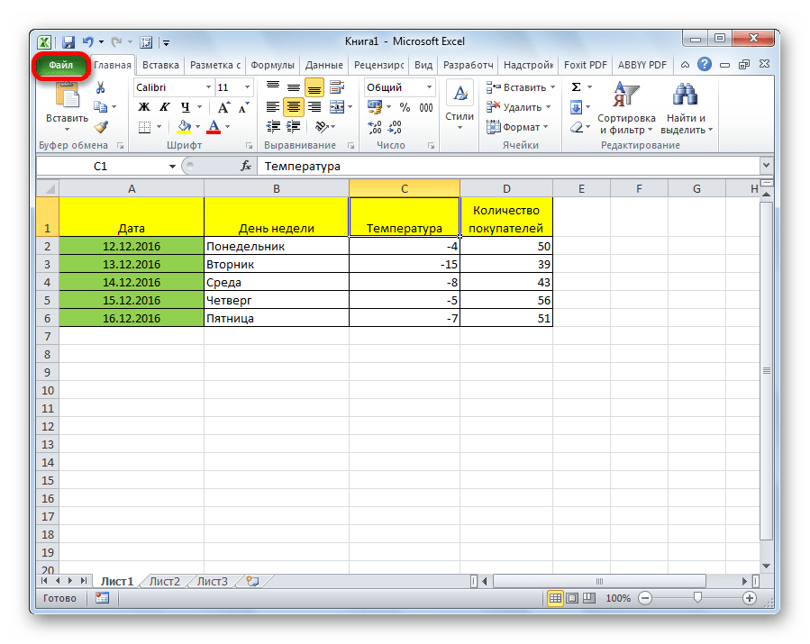
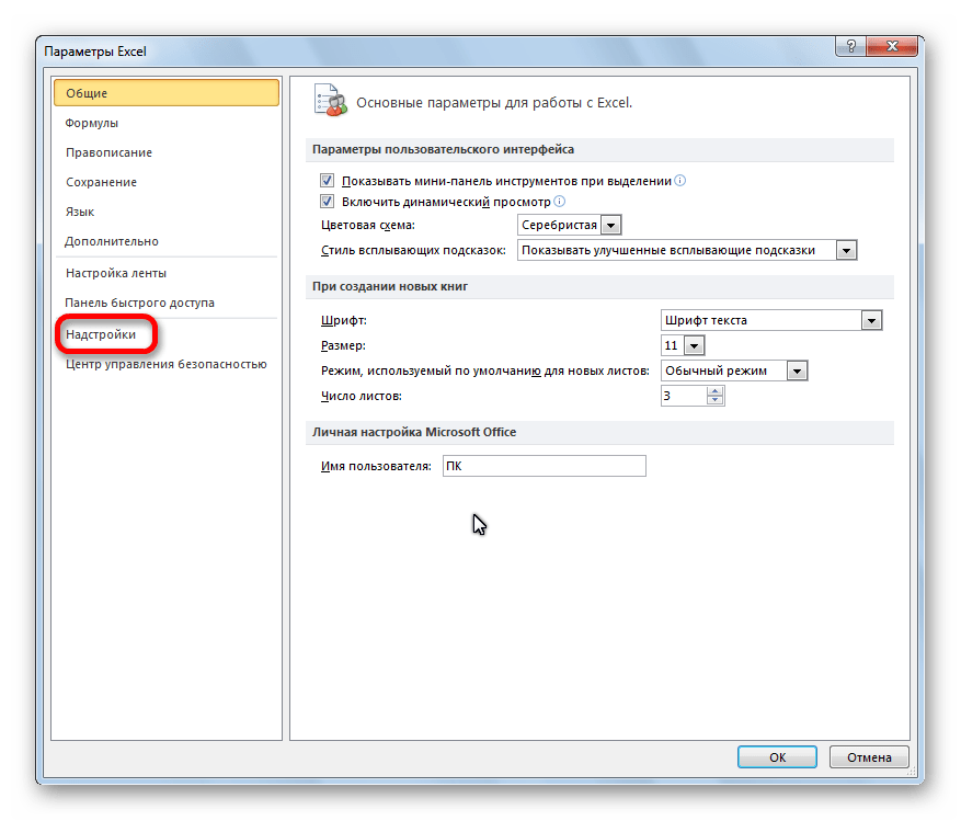
- Перемещаемся во вкладку «Файл».
- Переходим в раздел «Параметры».
- Открывается окно параметров Excel. Переходим в подраздел «Надстройки».
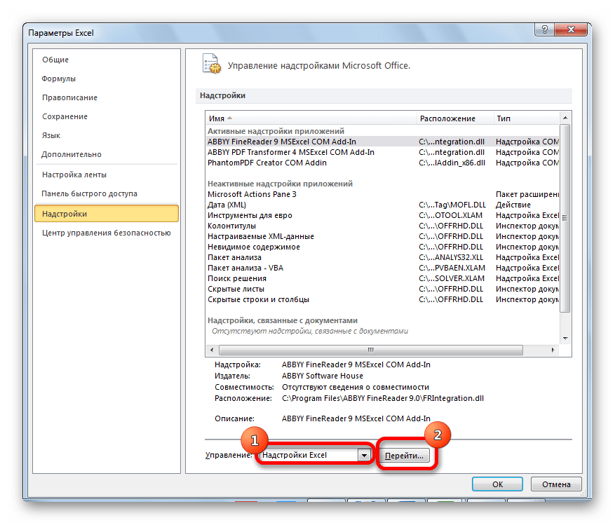
- В самой нижней части открывшегося окна переставляем переключатель в блоке «Управление» в позицию «Надстройки Excel», если он находится в другом положении. Жмем на кнопку «Перейти».
- Открывается окно доступных надстроек Эксель. Ставим галочку около пункта «Пакет анализа». Жмем на кнопку «OK».


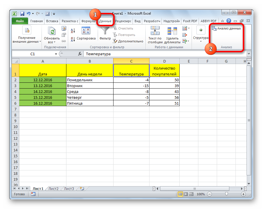
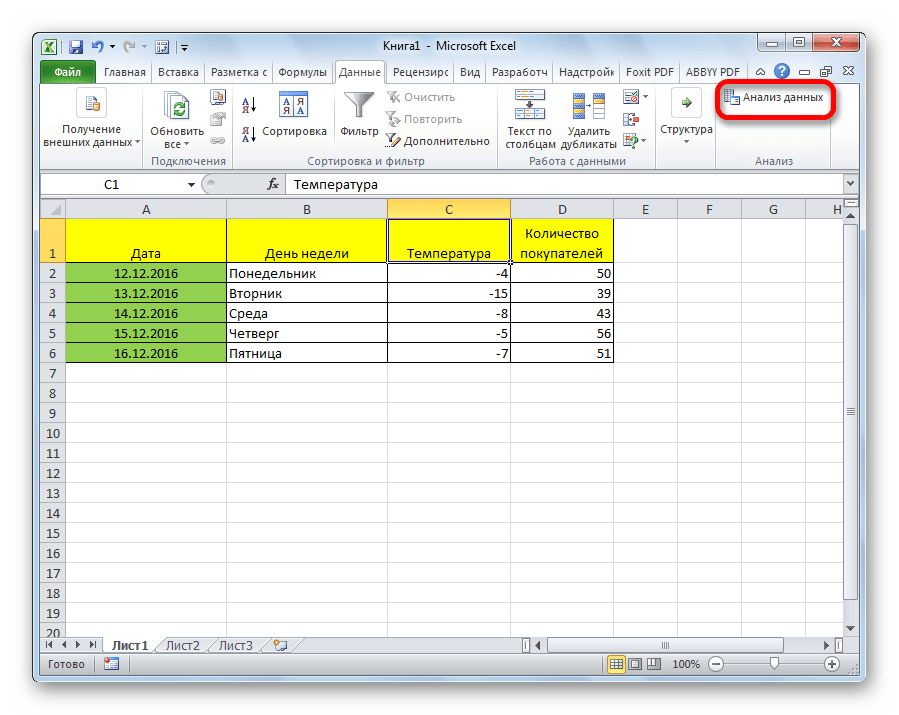
Теперь, когда мы перейдем во вкладку «Данные», на ленте в блоке инструментов «Анализ» мы увидим новую кнопку – «Анализ данных».
Виды регрессионного анализа
Существует несколько видов регрессий:
- параболическая;
- степенная;
- логарифмическая;
- экспоненциальная;
- показательная;
- гиперболическая;
- линейная регрессия.
О выполнении последнего вида регрессионного анализа в Экселе мы подробнее поговорим далее.
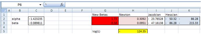
Внизу, в качестве примера, представлена таблица, в которой указана среднесуточная температура воздуха на улице, и количество покупателей магазина за соответствующий рабочий день. Давайте выясним при помощи регрессионного анализа, как именно погодные условия в виде температуры воздуха могут повлиять на посещаемость торгового заведения.
Общее уравнение регрессии линейного вида выглядит следующим образом: У = а0 + а1х1 +…+акхк. В этой формуле Y означает переменную, влияние факторов на которую мы пытаемся изучить. В нашем случае, это количество покупателей. Значение x – это различные факторы, влияющие на переменную. Параметры a являются коэффициентами регрессии. То есть, именно они определяют значимость того или иного фактора. Индекс k обозначает общее количество этих самых факторов.
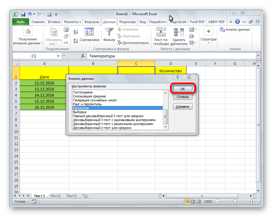
- Кликаем по кнопке «Анализ данных». Она размещена во вкладке «Главная» в блоке инструментов «Анализ».
- Открывается небольшое окошко. В нём выбираем пункт «Регрессия». Жмем на кнопку «OK».
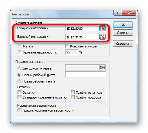
- Открывается окно настроек регрессии. В нём обязательными для заполнения полями являются «Входной интервал Y» и «Входной интервал X». Все остальные настройки можно оставить по умолчанию.
В поле «Входной интервал Y» указываем адрес диапазона ячеек, где расположены переменные данные, влияние факторов на которые мы пытаемся установить. В нашем случае это будут ячейки столбца «Количество покупателей». Адрес можно вписать вручную с клавиатуры, а можно, просто выделить требуемый столбец. Последний вариант намного проще и удобнее.
В поле «Входной интервал X» вводим адрес диапазона ячеек, где находятся данные того фактора, влияние которого на переменную мы хотим установить. Как говорилось выше, нам нужно установить влияние температуры на количество покупателей магазина, а поэтому вводим адрес ячеек в столбце «Температура». Это можно сделать теми же способами, что и в поле «Количество покупателей».

С помощью других настроек можно установить метки, уровень надёжности, константу-ноль, отобразить график нормальной вероятности, и выполнить другие действия. Но, в большинстве случаев, эти настройки изменять не нужно. Единственное на что следует обратить внимание, так это на параметры вывода. По умолчанию вывод результатов анализа осуществляется на другом листе, но переставив переключатель, вы можете установить вывод в указанном диапазоне на том же листе, где расположена таблица с исходными данными, или в отдельной книге, то есть в новом файле.
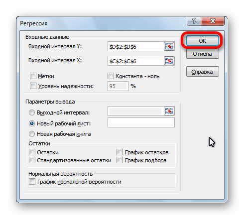
После того, как все настройки установлены, жмем на кнопку «OK».


Разбор результатов анализа
Результаты регрессионного анализа выводятся в виде таблицы в том месте, которое указано в настройках.
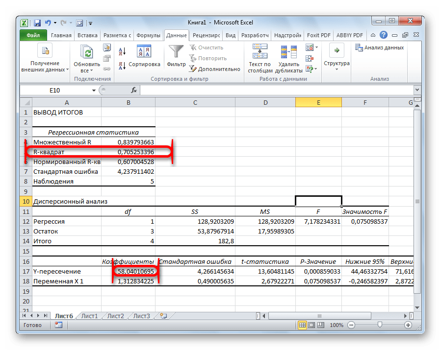
Одним из основных показателей является R-квадрат. В нем указывается качество модели. В нашем случае данный коэффициент равен 0,705 или около 70,5%. Это приемлемый уровень качества. Зависимость менее 0,5 является плохой.
Ещё один важный показатель расположен в ячейке на пересечении строки «Y-пересечение» и столбца «Коэффициенты». Тут указывается какое значение будет у Y, а в нашем случае, это количество покупателей, при всех остальных факторах равных нулю. В этой таблице данное значение равно 58,04.
Значение на пересечении граф «Переменная X1» и «Коэффициенты» показывает уровень зависимости Y от X. В нашем случае — это уровень зависимости количества клиентов магазина от температуры. Коэффициент 1,31 считается довольно высоким показателем влияния.
Как видим, с помощью программы Microsoft Excel довольно просто составить таблицу регрессионного анализа. Но, работать с полученными на выходе данными, и понимать их суть, сможет только подготовленный человек.
This is one of the following seven articles on Logistic Regression in Excel
Logistic Regression Overview
Logistic Regression in 7 Steps in Excel 2010 and Excel 2013
R Square For Logistic Regression Overview
Excel R Square Tests: Nagelkerke, Cox and Snell, and Log-Linear Ratio in Excel 2010 and Excel 2013
Likelihood Ratio Is Better Than Wald Statistic To Determine if the Variable Coefficients Are Significant For Excel 2010 and Excel 2013
Excel Classification Table: Logistic Regression’s Percentage Correct of Predicted Results in Excel 2010 and Excel 2013
Hosmer- Lemeshow Test in Excel – Logistic Regression Goodness-of-Fit Test in Excel 2010 and Excel 2013
The purpose of this example of binary logistic regression is to create an equation that will calculate the probability that a production machine is currently producing output that conforms to desired specifications based upon the age of the machine in months and the average number of shifts that the machine has operated during each week of its lifetime.
Data was collected on 20 similar machines as follows:
1) Whether the machine produces output that meets specifications at least 99 percent of the time.(1 = Machine Meets Spec – It Does Produce Conforming Output at least 99 Percent of the Time, 0 = Machine Does Not Meets Spec – It Does Not Produce Conforming Output at least 99 Percent of the Time)
2) The Machine’s Age in Months
3) The Average Number of Shifts That the Machine Has Operated Each Week During Its Lifetime.

(Click On Image To See a Larger Version)
Logistic Regression Steps in Excel
Logistic Regression Step 1 – Sort the Data
The purpose of sorting the data is to make data patterns more evident. Using Excel data sorting tool, perform the primary sort on the dependent variable. In this case, the dependent variable is the response variable indicating whether the prospect made a purchase. Perform subordinate sorts (secondary, tertiary, etc.) on the remaining variables.
The following data was sorted initially according to the response variable (Y). The secondary sort was done according to Machine Age and the tertiary sort was done according to Average Number of Shifts of Operation Per Week. The results are as follows:

(Click On Image To See a Larger Version)
Patterns are evident from the data sort. Machines that did not produce conforming output tended to the older machines and/or machines that operate during a higher average number of shifts per week.
Logistic Regression Step 2 – Calculate a Logit For Each Data Record
Given the following inputs, X1, X2, …, Xk, the Logit equals the following:
Logit = L = b0 + b1X1 + b2X2 + …+ bkXk
If the explanatory variables are Age and Average Number of Shifts, the Logit, L, is as follows:
Logit = L = b0 + b1*Age + b2*(Average Number of Weekly Shifts)
The Excel Solver will ultimately optimize the variables b0, b1, and b2 in order to create an equation that will accurately predict the probability of a machine producing conforming output given the machines age and average number of operating shifts per week.
The Decision Variables are the variables that the Solver adjusts during the optimization process. The Decision Variables b0, b1, and b2 are arbitrarily set to 0.1 before the Solver is run. It is a good idea to initially set the Solver decision variables so that the resulting Logit is well below 20 for each record. Logits that exceed 20 cause extreme values to occur in later steps of logistic regression. The Solver decision variables b0, b1, and b2 have been arbitrarily set to the value of 0.1 to initial produce reasonably small Logits as shown next.
A unique Logit is created for each of the 20 data records based on the initial settings of the Decision Variables as follows:
 (Click On Image To See a Larger Version)
Logistic Regression Step 3 – Calculate eL For Each Data Record
The number e is the base of the natural logarithm. It is approximately equal to 2.71828163 and is the limit of (1 + 1/n)n as n approaches infinity. eL must be calculated for each data record. This step will be shown in the image in the next step, Step 4.
Logistic Regression Step 4 – Calculate P(X) For Each Data Record
P(X) is the probability of event X occurring. Event X occurs when a machine produces conforming output. P(X) is the probability of a machine producing conforming output.
P(X) = eL / (1 + eL)
L = Logit = b0 + b1*X1 + b2*X2 + …+ bk*Xk
Calculating eL and P(X) for each of the data records is done as follows:
 (Click On Image To See a Larger Version)
eL can also be calculated in Excel as exp(L).
Logistic Regression Step 5 – Calculate LL, the Log-Likelihood Function
The conditional probability Pr(Yi=yi|X1i,X2i,…Xki) is the probability that predicted dependent variable yi equals the actual observed value Yi given the values of the independent variables inputs X1i,X2i,…Xki.
The conditional probability Pr(Yi=yi|X1i,X2i,…Xki) will be abbreviated Pr(Y=y|X) from here forward for convenience.
The conditional probability Pr(Y=y|X) is calculated by the following formula:
Pr(Y=y|X) = P(X)Y * [1-P(X)](1-Y)
Taking the natural log of both sides yields the following:
ln [ Pr(Y=y|X) ] = y*ln [ P(X) ] * (1-y)*ln[ [1-P(X)] ]
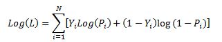
The Log-Likelihood Function, LL, is the sum of the ln [ Pr(Y=y|X) ] terms for all data records as per the following formula:
LL = ∑ Yi *P(Xi) + (1 – Yi)(1-P(Xi))
Calculating LL is done as follows:

(Click On Image To See a Larger Version)
 (Click On Image To See a Larger Version)
Logistic Regression Step 6 – Use the Excel Solver to Calculate MLL, the Maximum Log-Likelihood Function
The objective of Logistic Regression is find the coefficients of the Logit (b0 , b1,, b2 + …+ bk) that maximize LL, the Log-Likelihood Function in cell H30, to produce MLL, the Maximum Log-Likelihood Function.
The functionality of the Excel Solver is fairly straightforward: the Excel Solver adjusts the numeric values in specific cells in order to maximize or minimize the value in a single other cell.
The cell that the Solver is attempting to maximize or minimize is called the Solver Objective. This is LL in cell H30.
The cells whose values the Solver adjusts are called the Decision Variables. The Solver Decision Variables are therefore in cells C2, C3, and C4. These contain b0 , b1,, b2 + …+ bk, the coefficients of the Logit. These cells will be adjusted to maximize LL, which is in cell H30.
The Excel Solver is an add-in that in included with most Excel packages. The Solver most be manually activated by the user before it can be utilized for the first time. Different versions of Excel require different method of activation for the Solver. The best advice is to search Microsoft’s documentation online to locate instructions for activating the add-ins that are included with your version of Excel. YouTube videos are often another convenient source for step-by-step instructions for activating Solver in your version of Excel. Once activated, the Solver is normally found in the Data tab of versions of Excel from 2007 onward that use the ribbon navigation. Excel 2003 provides a link to the Solver in the drop-down menu under Tools.
These Decision Variables and Objective are entered into the Solver dialogue box as follows:
 (Click On Image To See a Larger Version)
Make sure not to check the checkbox next to Make Unconstrained Variables Non-Negative.
Excel Solver’s GRG Nonlinear Solving Method
The GRG Nonlinear solving method should be selected if any of the equations involving Decision variables or Constraints is nonlinear and smooth (uninterrupted, continuous, i.e., having no breaks). GRG stands for Generalized Reduced Gradient and is a long-time, proven, reliable method for solving nonlinear problems.
The equations on the path to the calculation of the Objective (maximizing LK) involve the calculation of eL, P(X), and Pr(Y=y|X). Each of these three equations is nonlinear and smooth. An equation is “smooth” if that equation and the derivative of that equation have no breaks (are continuous). The GRG Nonlinear solving method should therefore be selected.
One way to determine whether an equation or function is non-smooth (the graph has a sharp point indicating that the derivative is discontinuous) or discontinuous (the equation’s graph abruptly changes values at certain points – the graph is disconnected at these points) is to graph the equation over its expected range of values.
The Solver Should Be Run Through Several Trials To Ensure an Optimal Solution
When the Solver runs the GRG algorithm, it picks a starting point for its calculations. Each time the Solver GRG algorithm is run, it picks a slightly different starting point. This is why different answers will often appear after each run of the GRG Nonlinear solving method. The Solver should be re-run several times until the Objective (LK) is not maximized further. This should produce the best locally optimal values of the Decision Variables (b0, b1, b2, …, bk).
The GRG Nonlinear solving method is guaranteed to produce locally optimal solutions but not globally optimal solutions. The GRG nonlinear solving method will produce a Globally Optimal solution if all functions in the path to the Objective and all Constraints are convex. If any of the functions or Constraints is non-convex, the GRG Nonlinear solving method may find only Locally Optimal Solutions.
A function is convex if it has only one peak either up or down. A convex function can always be solved to a Globally Optimal solution. A function is non-convex if it has more than one peak or is discontinuous. Non-convex solutions can often be solved only to Locally Optimal solutions.
A Globally Optimal solution is the best possible solution that meets all Constraints. A Globally Optimal solution might be comparable to Mount Everest since Mount Everest is the highest of all mountains.
A Locally Optimal solution is the best nearby solution that meets all Constraints. It may not be the best overall solution, but it is the best nearby solution. A Locally Optimal solution might be comparable to Mount McKinley, which is the highest mountain in North America not the highest of all mountains.
The function eL with L = b0 + b1*X1 + b2*X2 + …+ bk*Xk can be non-convex because inputs X1 , X2 ,…, Xk can be nonlinear. The GRG Nonlinear solving method is therefore only guaranteed to find a Locally Optimal Solution.
How to Increase the Chance That the Solver Will Find a Globally Optimal Solution
There are three ways to increase the chance that the Solver will arrive at a Globally Optimal solution:
The first is to run the Solver multiple times using different sets of values for the Decision Variables. This option allows you to select initial sets of Decision Variables based on your understanding of the overall problem and is often the best way to arrive at the most desirable solution.
The second was is to select “Use Multistart.” This runs the GRG Solver for a number of times and randomly selects a different set of initial values for the Decision Variables during each run. The Solver then presents the best of all of the Locally Optimal solutions that it has found.
The third way is to set constraints in the Solver dialogue box that will force the Solver to try a new set of values. Constraints are limitations manually placed on the Decision Variables. Constraints can be useful if the Decision variables should be limited to a specific range of values. A Globally Optimal solution will not likely be found by applying constraints but a more realistic solution can be obtained by limiting Decision Variables to likely values.
Interpreting Excel Solver Results
Running the Solver produces the following results for this problem:

(Click On Image To See a Larger Version)
 (Click On Image To See a Larger Version)
MLL, the Maximum Log-Likelihood was calculated to be -6.654560484 when the constants were adjusted as Solver Decision Variables to the values of:
b0 = 12.48285608
b1 = -0.117031374
b2 = -1.469140055
Logistic Regression Step 7 – Test the Solver Output By Running Scenarios
Validate the output by running several scenarios through the Solver results. Each scenario will employ a different variation of input variables X1, X2, .. , Xk to produce outputs that should be consistent with the initial data set.
The sort of the initial data showed a pattern that nonconforming product was more likely on older machines and/or machines that were run more often.
The following three scenarios were run as follows:
Scenario 1
Machine Age = 40 months
Average Number of Weekly Shifts = 7
P(X) = Probability of Conforming Output = 8 percent
 (Click On Image To See a Larger Version)
Scenario 2
Machine Age = 40 months
Average Number of Weekly Shifts = 4
P(X) = Probability of Conforming Output = 87 percent
 (Click On Image To See a Larger Version)
Scenario 3
Machine Age = 12 months
Average Number of Weekly Shifts = 7
P(X) = Probability of Conforming Output = 69 percent
 (Click On Image To See a Larger Version)
The outcomes of these three scenarios are consistent with the patterns apparent in the initial sorted data set below that nonconforming product was more likely to be produced by older machines and/or machines that were run more often:

(Click On Image To See a Larger Version)
Excel Master Series Blog Directory
Statistical Topics and Articles In Each Topic
- Histograms in Excel
- Creating a Histogram With the Histogram Data Analysis Tool in Excel
- Creating an Automatically Updating Histogram in 7 Steps in Excel With Formulas and a Bar Chart
- Bar Chart in Excel
- Creating a Bar Chart in 7 Steps in Excel 2010 and Excel 2013
- Combinations & Permutations in Excel
- Combinations in Excel 2010 and Excel 2013
- Permutations in Excel 2010 and Excel 2013
- Normal Distribution in Excel
- Overview of the Normal Distribution
- Normal Distribution’s PDF (Probability Density Function) in Excel 2010 and Excel 2013
- Normal Distribution’s CDF (Cumulative Distribution Function) in Excel 2010 and Excel 2013
- Solving Normal Distribution Problems in Excel 2010 and Excel 2013
- Overview of the Standard Normal Distribution in Excel 2010 and Excel 2013
- An Important Difference Between the t and Normal Distribution Graphs
- The Empirical Rule and Chebyshev’s Theorem in Excel – Calculating How Much Data Is a Certain Distance From the Mean
- Demonstrating the Central Limit Theorem In Excel 2010 and Excel 2013 In An Easy-To-Understand Way
- t-Distribution in Excel
- Overview of the t- Distribution
- Binomial Distribution in Excel
- Overview of the Binomial Distribution in Excel 2010 and Excel 2013
- Solving Problems With the Binomial Distribution in Excel 2010 and Excel 2013
- Normal Approximation of the Binomial Distribution in Excel 2010 and Excel 2013
- Distributions Related to the Binomial Distribution
- z-Tests in Excel
- Overview of Hypothesis Tests Using the Normal Distribution in Excel 2010 and Excel 2013
- One-Sample z-Test in 4 Steps in Excel 2010 and Excel 2013
- 2-Sample Unpooled z-Test in 4 Steps in Excel 2010 and Excel 2013
- Overview of the Paired (Two-Dependent-Sample) z-Test in 4 Steps in Excel 2010 and Excel 2013
- t-Tests in Excel
- Overview of t-Tests: Hypothesis Tests that Use the t-Distribution
- 1-Sample t-Tests in Excel
- 1-Sample t-Test in 4 Steps in Excel 2010 and Excel 2013
- Excel Normality Testing For the 1-Sample t-Test in Excel 2010 and Excel 2013
- 1-Sample t-Test – Effect Size in Excel 2010 and Excel 2013
- 1-Sample t-Test Power With G*Power Utility
- Wilcoxon Signed-Rank Test in 8 Steps As a 1-Sample t-Test Alternative in Excel 2010 and Excel 2013
- Sign Test As a 1-Sample t-Test Alternative in Excel 2010 and Excel 2013
- 2-Independent-Sample Pooled t-Tests in Excel
- 2-Independent-Sample Pooled t-Test in 4 Steps in Excel 2010 and Excel 2013
- Excel Variance Tests: Levene’s, Brown-Forsythe, and F Test For 2-Sample Pooled t-Test in Excel 2010 and Excel 2013
- Excel Normality Tests Kolmogorov-Smirnov, Anderson-Darling, and Shapiro Wilk Tests For Two-Sample Pooled t-Test
- Two-Independent-Sample Pooled t-Test — All Excel Calculations
- 2- Sample Pooled t-Test – Effect Size in Excel 2010 and Excel 2013
- 2-Sample Pooled t-Test Power With G*Power Utility
- Mann-Whitney U Test in 12 Steps in Excel as 2-Sample Pooled t-Test Nonparametric Alternative in Excel 2010 and Excel 2013
- 2- Sample Pooled t-Test = Single-Factor ANOVA With 2 Sample Groups
- 2-Independent-Sample Unpooled t-Tests in Excel
- 2-Independent-Sample Unpooled t-Test in 4 Steps in Excel 2010 and Excel 2013
- Variance Tests: Levene’s Test, Brown-Forsythe Test, and F-Test in Excel For 2-Sample Unpooled t-Test
- Excel Normality Tests Kolmogorov-Smirnov, Anderson-Darling, and Shapiro-Wilk For 2-Sample Unpooled t-Test
- 2-Sample Unpooled t-Test Excel Calculations, Formulas, and Tools
- Effect Size for a 2-Independent-Sample Unpooled t-Test in Excel 2010 and Excel 2013
- Test Power of a 2-Independent Sample Unpooled t-Test With G-Power Utility
- Paired (2-Sample Dependent) t-Tests in Excel
- Paired t-Test in 4 Steps in Excel 2010 and Excel 2013
- Excel Normality Testing of Paired t-Test Data
- Paired t-Test Excel Calculations, Formulas, and Tools
- Paired t-Test – Effect Size in Excel 2010, and Excel 2013
- Paired t-Test – Test Power With G-Power Utility
- Wilcoxon Signed-Rank Test in 8 Steps As a Paired t-Test Alternative
- Sign Test in Excel As A Paired t-Test Alternative
- Hypothesis Tests of Proportion in Excel
- Hypothesis Tests of Proportion Overview (Hypothesis Testing On Binomial Data)
- 1-Sample Hypothesis Test of Proportion in 4 Steps in Excel 2010 and Excel 2013
- 2-Sample Pooled Hypothesis Test of Proportion in 4 Steps in Excel 2010 and Excel 2013
- How To Build a Much More Useful Split-Tester in Excel Than Google’s Website Optimizer
- Chi-Square Independence Tests in Excel
- Chi-Square Independence Test in 7 Steps in Excel 2010 and Excel 2013
- Chi-Square Goodness-Of-Fit Tests in Excel
- Overview of the Chi-Square Goodness-of-Fit Test
- Chi-Square Goodness- of-Fit Test With Pre-Determined Bins Sizes in 7 Steps in Excel 2010 and Excel 2013
- Chi-Square Goodness-Of-Fit-Normality Test in 9 Steps in Excel 2010 and Excel 2013
- F Tests in Excel
- F-Test in 6 Steps in Excel 2010 and Excel 2013
- Normality Testing For F Test In Excel 2010 and Excel 2013
- Levene’s and Brown- Forsythe Tests: F-Test Alternatives in Excel
- Correlation in Excel
- Overview of Correlation In Excel 2010 and Excel 2013
- Pearson Correlation in Excel
- Pearson Correlation in 3 Steps in Excel 2010 and Excel 2013
- Pearson Correlation – Calculating r Critical and p Value of r in Excel
- Spearman Correlation in Excel
- Spearman Correlation in 6 Steps in Excel 2010 and Excel 2013
- Confidence Intervals in Excel
- z-Based Confidence Intervals of a Population Mean in 2 Steps in Excel 2010 and Excel 2013
- t-Based Confidence Intervals of a Population Mean in 2 Steps in Excel 2010 and Excel 2013
- Minimum Sample Size to Limit the Size of a Confidence interval of a Population Mean
- Confidence Interval of Population Proportion in 2 Steps in Excel 2010 and Excel 2013
- Min Sample Size of Confidence Interval of Proportion in Excel 2010 and Excel 2013
- Simple Linear Regression in Excel
- Overview of Simple Linear Regression in Excel 2010 and Excel 2013
- Complete Simple Linear Regression Example in 7 Steps in Excel 2010 and Excel 2013
- Residual Evaluation For Simple Regression in 8 Steps in Excel 2010 and Excel 2013
- Residual Normality Tests in Excel – Kolmogorov-Smirnov Test, Anderson-Darling Test, and Shapiro-Wilk Test For Simple Linear Regression
- Evaluation of Simple Regression Output For Excel 2010 and Excel 2013
- All Calculations Performed By the Simple Regression Data Analysis Tool in Excel 2010 and Excel 2013
- Prediction Interval of Simple Regression in Excel 2010 and Excel 2013
- Multiple Linear Regression in Excel
- Basics of Multiple Regression in Excel 2010 and Excel 2013
- Complete Multiple Linear Regression Example in 6 Steps in Excel 2010 and Excel 2013
- Multiple Linear Regression’s Required Residual Assumptions
- Normality Testing of Residuals in Excel 2010 and Excel 2013
- Evaluating the Excel Output of Multiple Regression
- Estimating the Prediction Interval of Multiple Regression in Excel
- Regression — How To Do Conjoint Analysis Using Dummy Variable Regression in Excel
- Logistic Regression in Excel
- Logistic Regression Overview
- Logistic Regression in 6 Steps in Excel 2010 and Excel 2013
- R Square For Logistic Regression Overview
- Excel R Square Tests: Nagelkerke, Cox and Snell, and Log-Linear Ratio in Excel 2010 and Excel 2013
- Likelihood Ratio Is Better Than Wald Statistic To Determine if the Variable Coefficients Are Significant For Excel 2010 and Excel 2013
- Excel Classification Table: Logistic Regression’s Percentage Correct of Predicted Results in Excel 2010 and Excel 2013
- Hosmer- Lemeshow Test in Excel – Logistic Regression Goodness-of-Fit Test in Excel 2010 and Excel 2013
- Single-Factor ANOVA in Excel
- Overview of Single-Factor ANOVA
- Single-Factor ANOVA in 5 Steps in Excel 2010 and Excel 2013
- Shapiro-Wilk Normality Test in Excel For Each Single-Factor ANOVA Sample Group
- Kruskal-Wallis Test Alternative For Single Factor ANOVA in 7 Steps in Excel 2010 and Excel 2013
- Levene’s and Brown-Forsythe Tests in Excel For Single-Factor ANOVA Sample Group Variance Comparison
- Single-Factor ANOVA — All Excel Calculations
- Overview of Post-Hoc Testing For Single-Factor ANOVA
- Tukey-Kramer Post-Hoc Test in Excel For Single-Factor ANOVA
- Games-Howell Post-Hoc Test in Excel For Single-Factor ANOVA
- Overview of Effect Size For Single-Factor ANOVA
- ANOVA Effect Size Calculation Eta Squared in Excel 2010 and Excel 2013
- ANOVA Effect Size Calculation Psi – RMSSE – in Excel 2010 and Excel 2013
- ANOVA Effect Size Calculation Omega Squared in Excel 2010 and Excel 2013
- Power of Single-Factor ANOVA Test Using Free Utility G*Power
- Welch’s ANOVA Test in 8 Steps in Excel Substitute For Single-Factor ANOVA When Sample Variances Are Not Similar
- Brown-Forsythe F-Test in 4 Steps in Excel Substitute For Single-Factor ANOVA When Sample Variances Are Not Similar
- Two-Factor ANOVA With Replication in Excel
- Two-Factor ANOVA With Replication in 5 Steps in Excel 2010 and Excel 2013
- Variance Tests: Levene’s and Brown-Forsythe For 2-Factor ANOVA in Excel 2010 and Excel 2013
- Shapiro-Wilk Normality Test in Excel For 2-Factor ANOVA With Replication
- 2-Factor ANOVA With Replication Effect Size in Excel 2010 and Excel 2013
- Excel Post Hoc Tukey’s HSD Test For 2-Factor ANOVA With Replication
- 2-Factor ANOVA With Replication – Test Power With G-Power Utility
- Scheirer-Ray-Hare Test Alternative For 2-Factor ANOVA With Replication
- Two-Factor ANOVA Without Replication in Excel
- Two-Factor ANOVA Without Replication in Excel 2010 and Excel 2013
- Randomized Block Design ANOVA in Excel
- Randomized Block Design ANOVA in Excel 2010 and Excel 2013
- Repeated-Measures ANOVA in Excel
- Single-Factor Repeated-Measures ANOVA in 4 Steps in Excel 2010 and Excel 2013
- Sphericity Testing in 9 Steps For Repeated Measures ANOVA in Excel 2010 and Excel 2013
- Effect Size For Repeated-Measures ANOVA in Excel 2010 and Excel 2013
- Friedman Test in 3 Steps For Repeated-Measures ANOVA in Excel 2010 and Excel 2013
- ANCOVA in Excel
- Single-Factor ANCOVA in 8 Steps in Excel 2010 and Excel 2013
- Normality Testing in Excel
- Creating a Box Plot in 8 Steps in Excel
- Creating a Normal Probability Plot With Adjustable Confidence Interval Bands in 9 Steps in Excel With Formulas and a Bar Chart
- Chi-Square Goodness-of-Fit Test For Normality in 9 Steps in Excel
- Kolmogorov-Smirnov, Anderson-Darling, and Shapiro-Wilk Normality Tests in Excel
- Nonparametric Testing in Excel
- Mann-Whitney U Test in 12 Steps in Excel
- Wilcoxon Signed-Rank Test in 8 Steps in Excel
- Sign Test in Excel
- Friedman Test in 3 Steps in Excel
- Scheirer-Ray-Hope Test in Excel
- Welch’s ANOVA Test in 8 Steps Test in Excel
- Brown-Forsythe F Test in 4 Steps Test in Excel
- Levene’s Test and Brown-Forsythe Variance Tests in Excel
- Chi-Square Independence Test in 7 Steps in Excel
- Chi-Square Goodness-of-Fit Tests in Excel
- Chi-Square Population Variance Test in Excel
- Post Hoc Testing in Excel
- Tukey’s HSD Post Hoc Test in Excel
- Tukey-Kramer Post Hoc Test in Excel
- Games-Howell Post Hoc Test in Excel
- Creating Interactive Graphs of Statistical Distributions in Excel
- Interactive Statistical Distribution Graph in Excel 2010 and Excel 2013
- Interactive Graph of the Normal Distribution in Excel 2010 and Excel 2013
- Interactive Graph of the Chi-Square Distribution in Excel 2010 and Excel 2013
- Interactive Graph of the t-Distribution in Excel 2010 and Excel 2013
- Interactive Graph of the t-Distribution’s PDF in Excel 2010 and Excel 2013
- Interactive Graph of the t-Distribution’s CDF in Excel 2010 and Excel 2013
- Interactive Graph of the Binomial Distribution in Excel 2010 and Excel 2013
- Interactive Graph of the Exponential Distribution in Excel 2010 and Excel 2013
- Interactive Graph of the Beta Distribution in Excel 2010 and Excel 2013
- Interactive Graph of the Gamma Distribution in Excel 2010 and Excel 2013
- Interactive Graph of the Poisson Distribution in Excel 2010 and Excel 2013
- Solving Problems With Other Distributions in Excel
- Solving Uniform Distribution Problems in Excel 2010 and Excel 2013
- Solving Multinomial Distribution Problems in Excel 2010 and Excel 2013
- Solving Exponential Distribution Problems in Excel 2010 and Excel 2013
- Solving Beta Distribution Problems in Excel 2010 and Excel 2013
- Solving Gamma Distribution Problems in Excel 2010 and Excel 2013
- Solving Poisson Distribution Problems in Excel 2010 and Excel 2013
- Optimization With Excel Solver
- Maximizing Lead Generation With Excel Solver
- Minimizing Cutting Stock Waste With Excel Solver
- Optimal Investment Selection With Excel Solver
- Minimizing the Total Cost of Shipping From Multiple Points To Multiple Points With Excel Solver
- Knapsack Loading Problem in Excel Solver – Optimizing the Loading of a Limited Compartment
- Optimizing a Bond Portfolio With Excel Solver
- Travelling Salesman Problem in Excel Solver – Finding the Shortest Path To Reach All Customers
- Chi-Square Population Variance Test in Excel
- Overview of the Chi-Square Population Variance Test in Excel 2010 and Excel 2013
- Analyzing Data With Pivot Tables and Pivot Charts
- Simplifying Excel Pivot Table and Pivot Chart Setup
- SEO Functions in Excel
- Top 10 Excel SEO Functions — You’ll Like These
- Time Series Analysis in Excel
- Forecasting With Exponential Smoothing in Excel
- Forecasting With the Weighted Moving Average in Excel
- Forecasting With the Simple Moving Average in Excel
- VLOOKUP
- Simplifying Excel Lookup Functions: VLOOKUP, HLOOKUP, INDEX, MATCH, CHOOSE, and OFFSET
- VLOOKUP — Just Like Looking Up a Number in a Telephone Book
- VLOOKUP To Look Up a Discount in a Distant Database
Рассмотрим использование
MS
EXCEL
для прогнозирования переменной
Y
на основании нескольких переменных Х, т.е. множественную регрессию.
Перед прочтением этой статьи рекомендуется освежить в памяти
простую линейную регрессию
– прогнозирование на основе значений только одного фактора.
Disclaimer
: Данную статью не стоит рассматривать, как пересказ главы из учебника по статистике. Статья не обладает ни полнотой, ни строгостью изложения положений статистической науки. Эта статья – о применении MS EXCEL для целей
Множественного регрессионного анализа.
Теоретические отступления приведены лишь из соображения логики изложения. Использование данной статьи для изучения
Регрессии
– плохая идея.
Статья про
Множественный регрессионный анализ
получилась большая, поэтому ниже для удобства приведены ее разделы:
- Оценка неизвестных параметров
- Диаграмма рассеяния
-
Вычисление прогнозных значений Y
(отдельное наблюдение и среднее значение) и построение доверительных интервалов
- Стандартные ошибки и доверительные интервалы для коэффициентов регрессии
- Проверка гипотез
- Генерация данных для множественной регрессии с помощью заданного тренда
- Коэффициент детерминации
Прогнозирование единственной переменной Y на основании значений 2-х или более переменных Х называется
множественной регрессией
.
Множественная линейная регрессионная модель
(Multiple Linear Regression Model)
имеет вид Y=β
0
+β
1
*X
1
+β
2
*X
2
+…+β
k
*X
k
+ε. В этом случае переменная Y зависит от k поясняющих переменных Х, т.е.
регрессоров
. ε —
случайная ошибка
. Модель является линейной относительно неизвестных параметров β.
Оценка неизвестных параметров
В этой статье рассмотрим модель с 2-мя регрессорами. Сначала введем необходимые обозначения и понятия множественной регрессии.
Для описания зависимости Y от 2-х переменных
линейная модель
имеет вид:
Y=β
0
+β
1
*X
1
+β
2
*X
2
+ε.
Параметры этой модели β
i
нам неизвестны, но их можно оценить, используя случайную выборку (измеренные значения переменной Y от заданных Х). Оценки параметров модели (β
0
, β
1
, β
2
) обычно вычисляются
методом наименьших квадратов (МНК)
, который минимизирует сумму квадратов ошибок прогнозирования (критерий минимизации в англоязычной литературе обозначают как SSE – Sum of Squared Errors).
Соответствующие оценки параметров будем обозначать как
b
0
,
b
1
и
b
2
.
Ошибка ε имеет случайную природу и имеет свою функцию распределения со
средним значением
=0 и
дисперсией σ
2
.
Оценки
b
1
и
b
2
называются
коэффициентами регрессии
, они определяют влияние соответствующей переменной X, когда все остальные независимые переменные остаются
неизменными
.
Сдвиг (intercept)
или
постоянный
член
b
0
, определяет прогнозируемое значение Y, когда все поясняющие переменные Х равны 0 (часто
сдвиг
не имеет физического смысла в рамках модели и обусловлен лишь математическими вычислениями
МНК
).
Вычислив оценки, полученные методом
МНК,
позволяют прогнозировать значения переменной Y:
Y=
b
0
+
b
1
*X
1
+
b
2
*X
2
Примечание
: Для случая 2-х регрессоров, все спрогнозированные значения переменной Y будут лежать в плоскости (в
плоскости регрессии
).
В качестве примера рассмотрим технологический процесс изготовления нити:
Инженер, на основе имеющегося опыта, предположил, что
прочность нити
Y зависит от
концентрации исходного раствора
(Х
1
) и
температуры реакции
(Х
2
), и соответствует модели линейной регрессии. Для нахождения комбинации переменных Х, при которых Y принимает максимальное значение, необходимо определить коэффициенты регрессии, сделав выборку.
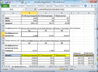
В MS EXCEL
коэффициенты множественной регрессии
удобнее всего вычислить с помощью функции
ЛИНЕЙН()
. Это сделано в
файле примера на листе Коэффициенты
. Чтобы вычислить оценки:
-
выделите 3 ячейки в одной строке (т.к. мы рассматриваем случай 2-х регрессоров, то будут вычислены 2
коэффициента регрессии
+
величина сдвига
= 3 значения, для вывода которых понадобится 3 ячейки). Пусть это будет диапазон
С8:Е8
; -
в
Строке формул
введите =
ЛИНЕЙН(D20:D50;B20:C50)
. Предполагается, что в столбце
В
содержатся прогнозируемые значения Y (в нашей модели это Прочность нити), в столбцах
С
и
D
содержатся значения контролируемых параметров Х (Х1 – Концентрация в столбце С и Х2 – Температура в столбце D). -
нажмите
CTRL
+
SHIFT
+
ENTER
(т.к. этоформула массива
).
В левой ячейке будет рассчитано значение
коэффициента регрессии
b
2
для переменной Х2, в средней ячейке — значение
коэффициента регрессии
b
1
для переменной Х1, в правой –
сдвиг
. Обратите внимание, что порядок вывода
коэффициентов
регрессии
обратный по отношению к расположению столбцов с данными соответствующих переменных Х (вычисленный коэффициент
b
2
располагается
левее
по отношению к
b
1
, тогда как значения переменной Х2 располагаются
правее
значений переменной Х1). Это может привести к путанице, поэтому лучше разместить коэффициенты над соответствующими столбцами с данными, как это сделано в строке 17
файла примера
.
Примечание
: В принципе без функции
ЛИНЕЙН()
можно обойтись, записав альтернативные формулы. Для этого в
файле примера на листе Коэффициенты
в столбцах
I
:
K
вычислены отклонения значений переменных Х
1i
, Х
2i
, Y
i
от их средних значений
![]()
, т.е.:
![]()
Далее коэффициенты регрессии рассчитываются по следующим формулам (эти формулы справедливы только при прогнозировании по 2-м независимым переменным Х):
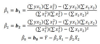
При прогнозировании по 3-м и более независимым переменным Х формулы для вычисления
коэффициентов регрессии
значительно усложняются, поэтому следует использовать матричный подход.
В
файле примера на листе Матричная форма
выполнены расчеты
коэффициентов регрессии
с помощью матричного подхода.
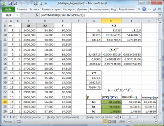
Расчет можно произвести как пошагово, так и одной
формулой массива
:
=МУМНОЖ(МОБР(МУМНОЖ(ТРАНСП(B9:D33);(B9:D33)));МУМНОЖ(ТРАНСП(B9:D33);(E9:E33)))
Коэффициенты регрессии
(вектор
b
)
в этом случае вычисляются по формуле
b
=(X
T
X)
-1
(X
T
Y) или в другом виде записи
b
=(X
’
X)
-1
(X
’
Y)
Под Х подразумевается матрица, состоящая из столбцов значений переменной Х с дополнительным столбцом единиц, а под Y – вектор-столбец значений Y.
Символ
Т
или ‘ – это
транспонирование матрицы
, а обозначение
-1
говорит о
вычислении обратной матрицы
.
Диаграмма рассеяния
В случае
простой линейной регрессии
(один регрессор, т.е. одна переменная Х) для визуализации связи между прогнозируемым значением Y и переменной Х строят
диаграмму рассеяния
(двумерную).

В случае
множественной
линейной регрессии
двумерную диаграмму рассеяния можно построить только для анализа влияния каждого отдельного регрессора на Y (при этом остальные Х не меняются), т.е. так называемую Матричную диаграмму рассеивания (См.
файл примера лист Диагр расс (матричная)
).
К сожалению, такую диаграмму трудно интерпретировать.
Более того, матричная диаграмма может вводить в заблуждение (см.
Introduction
to
linear
regression
analysis
/
D
.
C
.
Montgomery
,
E
.
A
.
Peck
,
G
.
G
.
Vining
, раздел 3.2.5
), демонстрируя наличие или отсутствие линейной взаимосвязи между отдельным регрессором X
i
и Y.
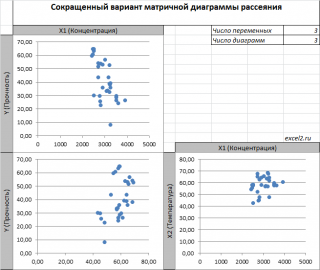
Для случая с 2-мя регрессорами можно предложить альтернативный вид матричной
диаграммы рассеяния
. В стандартной диаграмме рассеяния строятся проекции на координатные плоскости Х1;Х2, Y;X1 и Y;X2. Однако, если взглянуть на точки относительно
плоскости регрессии
, то картину, на мой взгляд, будет проще интерпретировать.
Сравним две матричные диаграммы рассеяния (см.
файл примера на листе «Диагр расс (в плоск регрессии)»
, построенные для одних и тех же наблюдений. Первая – стандартная,
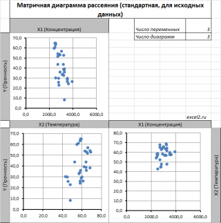
вторая представляет собой вид сверху на плоскость регрессии и 2 вида вдоль плоскости.
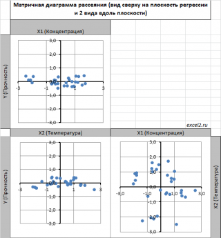
На второй диаграмме становится очевидно, что разброс точек относительно плоскости регрессии совсем не большой и поэтому, скорее всего, построенная модель является полезной, а выбранные 2 переменные Х позволяют прогнозировать Y (конечно, для подтверждения этой гипотезы нужно
провести процедуру F-теста
).
Несколько слов о построении альтернативной матричной диаграммы рассеяния:
-
Перед построением необходимо нормировать значения наблюдений (для каждой переменной вычесть
среднее
и разделить на
стандартное отклонение
). В этом случае практически все точки на диаграммах будут находится в диапазоне +/-3 (по аналогии со
стандартным нормальным распределением
, 99% значений которого лежат в пределах +/-3 сигма). В этом случае, на диаграмме можно фиксировать мин/макс значений осей, чтобы EXCEL автоматически не модифицировал масштаб осей при изменении данных (это не всегда удобно);
-
Теперь координаты точек необходимо рассчитать в системе отсчета относительно плоскости регрессии (в которой плоскость Оху’ совпадает с плоскостью регрессии). Для этого необходимо найти
матрицу вращения
, например, через вращение приводящее к совмещению нормали к плоскости регрессии и вектора оси Z (0;0;1);
-
Новые координаты позволяют построить альтернативную матричную диаграмму. Кроме того, для удобства можно вращать систему координат вокруг новой оси Z, чтобы нагляднее представить себе распределение точек относительно плоскости регрессии (для этого использована Полоса прокрутки в ячейках
Q
31:
S
31
).
Вычисление прогнозных значений Y (отдельное наблюдение и среднее значение) и построение доверительных интервалов
После того, как нами были найдены тем или иным способом коэффициенты регрессии можно приступать к вычислению прогнозных значений Y на основе заданных значений переменных Х.
Уравнение прогнозирования или уравнение регрессии в случае 2-х независимых переменных (регрессоров) записывается в виде:
Y=
b
0
+
b
1
*
Х
1
+
b
2
*
Х
2
Примечание:
В MS EXCEL
прогнозное значение Y для заданных Х
1
и Х
2
можно также предсказать с помощью функции
ТЕНДЕНЦИЯ()
. При этом 2-й аргумент будет ссылкой на столбцы, содержащие все значения переменных Х
1
и Х
2
, а 3-й аргумент функции должен быть ссылкой на диапазон ячеек, содержащий 2 значения Х (Х
1i
и Х
2i
) для выбранного наблюдения i (см.
файл примера, лист Коэффициенты, столбец G
). Функция
ПРЕДСКАЗ()
, использованная нами в простой регрессии, не работает в случае
множественной регрессии
.
Найдя прогнозное значение Y, мы, таким образом, вычислим его точечную оценку. Понятно, что фактическое значение Y, полученное при наблюдении, будет, скорее всего, отличаться от этой оценки. Чтобы ответить на вопрос о том, на сколько хорошо мы можем предсказывать новые значения Y, нам потребуется построить
доверительный интервал
этой оценки, т.е. диапазон в котором с определенной заданной вероятностью, скажем 95%, мы ожидаем новое значение Y.
Доверительные интервалы
построим при фиксированном Х для:
- нового наблюдения Y;
- среднего значения Y (интервал будет уже, чем для отдельного нового наблюдения)
Как и в случае
простой линейной регрессии
, для построения
доверительных интервалов
нам потребуется сначала вычислить
стандартную ошибку модели
(standard error of the model)
, которая приблизительно показывает насколько велика ошибка предсказания значений переменной Y на основании значений переменных Х.
Для вычисления
стандартной ошибки
оценивают
дисперсию
ошибки ε, т.е. сигма^2
(ее часто обозначают как
MS
Е либо
MSres
)
. Затем, вычислив из полученной оценки квадратный корень, получим
Стандартную ошибку регрессии (часто обозначают как
SEy
или
sey
).
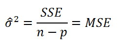
где SSE – сумма квадратов значений ошибок модели ei=yi — ŷi (
Sum of Squared Errors
). MSE означает Mean Square of Errors (среднее квадратов ошибок, точнее остатков).
Величина n-p – это количество
степеней свободы
(
df
–
degrees
of
freedom
), т.е. число параметров системы, которые могут изменяться независимо (вспомним, что у нас в этом примере есть n независимых наблюдений переменной Y, р – количество оцениваемых параметров модели). В случае
простой множественной регрессии
с 2-мя регрессорами
число степеней свободы
равно n-3, т.к. при построении
плоскости регрессии
было оценено 3 параметра модели
b
(т.е. на это было «потрачено» 3
степени свободы
).
В MS EXCEL
стандартную ошибку
SEy можно вычислить формулы (см.
файл примера, лист Статистика
):
=
ИНДЕКС(ЛИНЕЙН($E$13:$E$43;$C$13:$D$43;;ИСТИНА);3;2)
Стандартная ошибка
нового наблюдения Y при заданных значениях Х (вектор Хi) вычисляется по формуле:
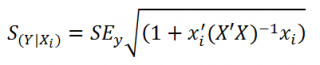
x
i
— вектор-столбец со значениями переменных Х (с дополнительной 1) для заданного наблюдения i.
Соответствующий доверительный интервал вычисляется по формуле:
![]()
где α (альфа) –
уровень значимости
(обычно принимают равным 0,05=5%)
р – количество оцениваемых параметров модели (в нашем случае = 3)
n-p – число степеней свободы

–
квантиль
распределения Стьюдента
(задает количество
стандартных ошибок
, в +/- диапазоне которых вероятность обнаружить новое наблюдение равно 1-альфа). Т.е. если
квантиль
равен 2, то диапазон шириной +/- 2
стандартных ошибок
относительно прогнозного значения Y будет с вероятностью 95% содержать новое наблюдение Y (для каждого заданного Хi). В MS EXCEL вычисления квантиля производят по формуле =
СТЬЮДЕНТ.ОБР.2Х(0,05;n-p)
, подробнее см.
в статье про распределение Стьюдента
.
![]()
– прогнозное значение Yi вычисляемое по формуле Yi=
b
0+
b
1*
Х1i+
b
2*
Х2i (точечная оценка).
Стандартная ошибка
среднего значения Y при заданных значениях Х (вектор Хi) будет меньше, чем стандартная ошибка отдельного наблюдения. Вычисления производятся по формуле:
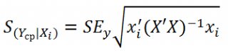
x
i
— вектор-столбец со значениями переменных Х (с дополнительной 1) для заданного наблюдения i.
Соответствующий
доверительный интервал
вычисляется по формуле:
![]()
Прогнозное значение Yi (точечная оценка) используется тоже, что и для отдельного наблюдения.
Стандартные ошибки и доверительные интервалы для коэффициентов регрессии
В разделе
Оценка неизвестных параметров
мы получили точечные оценки
коэффициентов регрессии
. Так как эти оценки получены на основе случайных величин (значений переменных Х и Y), то эти оценки сами являются случайными величинами и соответственно имеют функцию распределения со
средним значением
и
дисперсией
. Но, чтобы перейти от
точечных оценок
к
интервальным
, необходимо вычислить соответствующие
стандартные ошибки
(т.е.
стандартные отклонения
)
коэффициентов регрессии
.
Стандартная ошибка коэффициента регрессии
b
j
(обозначается
se
(
b
j
)
) вычисляется на основании
стандартной ошибки
по следующей формуле:
где C
jj
является диагональным элементом матрицы (X
’
X)
-1
. Для коэффициента сдвига
b
0
индекс j=1 (верхний левый элемент), для
b
1
индекс j=2,
b
2
индекс j=3 (нижний правый элемент).
SEy –
стандартная ошибка регрессии
(см.
выше
).
В MS EXCEL
стандартные ошибки коэффициентов регрессии
можно вычислить с помощью функции
ЛИНЕЙН()
:
=
ИНДЕКС(ЛИНЕЙН($E$13:$E$43;$C$13:$D$43;;ИСТИНА);2;j)
Примечание
: Подробнее о функции
ЛИНЕЙН()
см. статью
Функция MS EXCEL ЛИНЕЙН()
.
Применяя матричный подход
стандартные ошибки
можно вычислить и через обычные формулы (точнее через
формулу массива
, см.
файл примера лист Статистика
):
=
КОРЕНЬ(СУММКВРАЗН(E13:E43;F13:F43) /(n-p)) *КОРЕНЬ (ИНДЕКС (МОБР (МУМНОЖ(ТРАНСП(B13:D43);(B13:D43)));j;j))
При построении
двухстороннего доверительного интервала
для
коэффициента регрессии
его границы определяются следующим образом:
b
j
+/- t*Se(
b
j
)
где t – это
t-значение
, которое можно вычислить с помощью формулы =
СТЬЮДЕНТ.ОБР.2Х(0,05;n-p)
для
уровня значимости
0,05.
В результате получим, что найденный
доверительный интервал
с вероятностью 95% (1-0,05) накроет истинное значение
коэффициента регрессии
b
j
.
Здесь мы считаем, что
коэффициент регрессии
b
j
имеет
распределение Стьюдента
с n-p
степенями свободы
(n – количество наблюдений, т.е. пар Х и Y).
Проверка гипотез
Когда мы строим модель, мы предполагаем, что между Y и переменными X существует линейная взаимосвязь. Однако, как это иногда бывает в статистике, можно вычислять параметры связи даже тогда, когда в действительности она не существует, и обусловлена лишь случайностью.
Единственный вариант, когда Y не зависит X, возможен, когда все
коэффициенты регрессии
β
равны 0.
Чтобы убедиться, что вычисленная нами оценка
коэффициентов регрессии
не обусловлена лишь случайностью (они не случайно отличны от 0), используют
проверку гипотез
. В качестве
нулевой гипотезы
Н
0
принимают, что линейной связи нет, т.е. ВСЕ β=0. В качестве альтернативной гипотезы
Н
1
принимают, что ХОТЯ БЫ ОДИН коэффициент β <>0.
Процедура проверки значимости множественной регрессии, приведенная ниже, является обобщением
дисперсионного анализа
, использованного нами в случае
простой линейной регрессии (F-тест)
.
Если нулевая гипотеза справедлива, то
тестовая
F
-статистика
имеет
F-распределение
со степенями свободы
k
и
n
—
k
-1
, т.е. F
k, n-k-1
:
Проверку значимости регрессии можно также осуществить через вычисление
p
-значения
. В этом случае вычисляют вероятность того, что случайная величина F примет значение F
0
(это и есть
p-значение
), затем сравнивают p-значение с заданным
уровнем значимости α (альфа)
. Если
p-значение
больше уровня значимости
,
то нулевую гипотезу нет оснований отклонить, и регрессия незначима.
В MS EXCEL значение F
0
можно вычислить на основании значений выборки по вышеуказанной формуле или с помощью функции
ЛИНЕЙН()
:
=
ИНДЕКС(ЛИНЕЙН(E13:E43; C13:D43;;ИСТИНА);4;1)
В MS EXCEL для проверки гипотезы через
p
-значение
используйте формулу =F.РАСП.ПХ(F
0
;k;n-k-1)<
альфа
Если формула вернет ИСТИНА, то регрессия значима. Если формула вернет ЛОЖЬ, то у нас нет оснований отклонить нулевую гипотезу, т.е. «скорее всего» все коэффициенты регрессии равны 0 (см.
файл примера лист Статистика
, где показано эквивалентность обоих подходов проверки значимости регрессии).

В MS EXCEL критическое значение для заданного
уровня значимости
F
1-альфа, k, n-k-1
можно вычислить по формуле =
F.ОБР(1- альфа;k;n-k-1)
или =
F.ОБР.ПХ(альфа;k; n-k-1)
. Другими словами требуется вычислить
верхний альфа-
квантиль
F
-распределения
с соответствующими
степенями свободы
.
Таким образом, при значении статистики F
0
> F
1-альфа, k, n-k-1
мы имеем основание для отклонения нулевой гипотезы.
В программах статистики результаты процедуры
F
-теста
выводят с помощью стандартной таблицы
дисперсионного анализа
. В
файле примера такая таблица приведена на листе Надстройка
, которая построена на основе результатов, возвращаемых инструментом
Регрессия надстройки Пакета анализа MS EXCEL
.
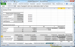
Генерация данных для множественной регрессии с помощью заданного тренда
Иногда, бывает удобно сгенерировать значения наблюдений, имея заданный тренд.
Для решения этой задачи нам потребуется:
- задать значения регрессоров в нужном диапазоне (значения переменных Х);
-
задать коэффициенты регрессии (
b
); -
задать тренд (вычислить значения Y=
b
0
+
b
1
*
Х
1
+
b
2
*
Х
2
); - задать величину разброса Y вокруг тренда (варианты: случайный разброс в заданных границах или заданная фигура, например, круг)
Все вычисления выполнены в
файле примера, лист Тренд
для случая 2-х регрессоров. Там же построены
диаграммы рассеяния
.
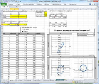
Коэффициент детерминации
Коэффициент детерминации
R
2
показывает насколько полезна построенная нами
линейная регрессионная модель
.
По определению
коэффициент детерминации
R
2
равен:
R
2
=
Изменчивость объясненная моделью (
SSR
) / Общая изменчивость (
SST
).
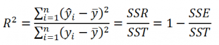
Этот показатель можно вычислить с помощью функции
ЛИНЕЙН()
:
=
ИНДЕКС(ЛИНЕЙН(E13:E43;C13:D43;;ИСТИНА);3)
При добавлении в модель новой объясняющей переменной Х,
коэффициент детерминации
будет всегда расти. Поэтому, рост
коэффициента детерминации
не может служить основанием для вывода о том, что новая модель (с дополнительным регрессором) лучше прежней.
Более подходящей статистикой, которая лишена указанного недостатка, является
нормированный
коэффициент детерминации
(Adjusted R-squared):
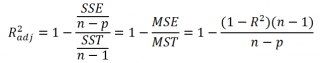
где p – число независимых
регрессоров
(вычисления см.
файл примера лист Статистика
).