
Suppose that your boss wants you to protect an entire workbook, but also wants to be able to change a few cells after you enable protection on the workbook. Before you enabled password protection, you had unlocked some cells in the workbook. Now that your boss is done with the workbook, you can lock these cells.
Follow these steps to lock cells in a worksheet:
-
Select the cells you want to lock.
-
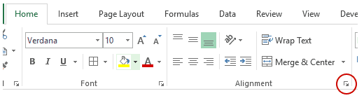
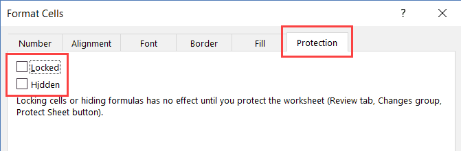
On the Home tab, in the Alignment group, click the small arrow to open the Format Cells popup window.
-
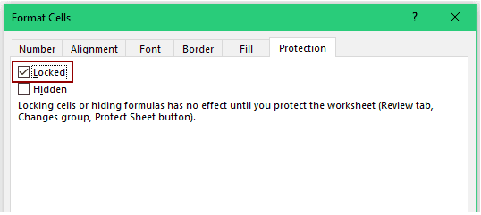
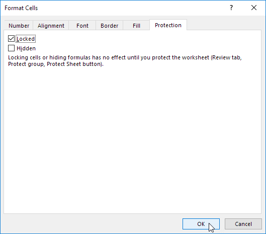
On the Protection tab, select the Locked check box, and then click OK to close the popup.
Note: If you try these steps on a workbook or worksheet you haven’t protected, you’ll see the cells are already locked. This means that the cells are ready to be locked when you protect the workbook or worksheet.
-
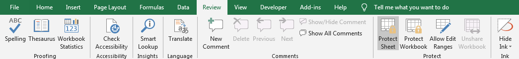
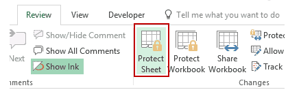
On the Review tab in the ribbon, in the Changes group, select either Protect Sheet or Protect Workbook, and then reapply protection. See Protect a worksheet or Protect a workbook.
Tip: It’s a best practice to unlock any cells that you may want to change before you protect a worksheet or a workbook, but you can also unlock them after you apply protection. To remove protection, simply remove the password.
In addition to protecting workbooks and worksheets, you can also protect formulas.
Excel for the web can’t lock cells or specific areas of a worksheet.
If you want to lock cells or protect specific areas, click Open in Excel and lock cells to protect them or lock or unlock specific areas of a protected worksheet.
![]()
Download Article
![]()
Download Article
Locking cells in an Excel spreadsheet can prevent any changes from being made to the data or formulas that reside in those particular cells. Cells that are locked and protected can be unlocked at any time by the user who initially locked the cells. Follow the steps below to learn how to lock and protect cells in Microsoft Excel versions 2010, 2007, and 2003.
To learn how to unlock the cells, read the article How to Open a Password Protected Excel File.
Things You Should Know
- In all versions of Excel, highlight and right click your cells. Then, select «Format Cells» > «Protection.» Check «Locked» and save.
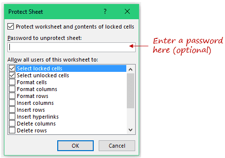
- In Excel 2007 and 2010, go to «Review» > «Changes/Protect Sheet» > «Protect worksheet and contents of locked cells.» Type a password click through the prompts to save.
- In Excel 2003, go to «Tools» > «Protection» > «Protect Sheet.» Check «Protect worksheet and contents of locked cells.» Enter a password and follow the prompts to save.
-

1
Open the Excel spreadsheet that contains the cells you want locked.
-
2
Select the cell or cells you want locked.
Advertisement
-
3
Right-click on the cells, and select «Format Cells.»
-
4
Click on the tab labeled «Protection.»
-
5
Place a checkmark in the box next to the option labeled «Locked.»
-
6
Click «OK.»
-
7
Click on the tab labeled «Review» at the top of your Excel spreadsheet.
-
8
Click on the button labeled «Protect Sheet» from within the «Changes» group.
-
9
Place a checkmark next to «Protect worksheet and contents of locked cells.»
-
10
Enter a password in the text box labeled «Password to unprotect sheet.»
-
11
Click on «OK.»
-
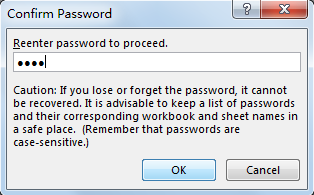
12
Retype your password into the text box labeled «Reenter password to proceed.»
-
13
Click «OK.» The cells you selected will now be locked and protected, and can only be unlocked by selecting the cells once again, and entering the password you selected.


Advertisement
-
1
Open the Excel document that contains the cell or cells you want to lock.
-
2
Select one or all of the cells you want locked.
-
3
Right-click on your cell selections, and select «Format Cells» from the drop-down menu.
-
4
Click on the «Protection» tab.
-
5
Place a checkmark next to the field labeled «Locked.»
-
6
Click the «OK» button.
-
7
Click on the «Tools» menu at the top of your Excel document.
-
8
Select «Protection» from the list of options.
-
9
Click on «Protect Sheet.»
-
10
Place a checkmark next to the option labeled «Protect worksheet and contents of locked cells.»
-
11
Type a password at the prompt for «Password to unprotect sheet,» then click «OK.»
-
12
Reenter your password at the prompt for «Reenter password to proceed.»
-
13
Select «OK.» All the cells you selected will now be locked and protected, and can only be unlocked going forward by selecting the locked cells, and entering the password you initially set up.


Advertisement
Add New Question
-
Question
How do I lock cells in Excel without the whole document becoming read only?

I suppose you want to lock certain cells instead of the whole sheets. To do that, choose the whole sheet, right click and then select «Format Cells», then «Protection», then uncheck the «Locked» option and click okay. Then select the cells you want to lock, right click and select «Format Cells», then Protection; this time, check the «Locked» option and click okay. Now go back to the main tab, select «Review», then click on «Protect Sheet», and do whatever you want to do with it. Now only the cells you «locked» are protected from editing instead of the whole sheet.
-
Question
How can I protract the single cell while using Excel?
You cannot protract a single cell in Excel. You can, however, make it appear longer than the rest of the cells around it by «merging» two or more cells together. Highlight the cells you desire and right click. A menu will pop up allowing you to merge them.
-
Question
How do I allow changes to some cells of a protected sheet?
Select the whole worksheet by clicking the Select All button. On the Home tab, in the Font group, click the Format Cell Font dialog box launcher. On the Protection tab, clear the Locked box and then click OK.
Ask a Question
200 characters left
Include your email address to get a message when this question is answered.
Submit
Advertisement
Video
-
If multiple users have access to your Excel document, lock all cells that contain important data or complex formulas to prevent the cells from being accidentally changed.
-
If the majority of cells in your Excel document contain valuable data or complex formulas, consider locking or protecting the entire document, then unlock the few cells that are allowed to be modified.
Thanks for submitting a tip for review!
Advertisement
About This Article
Article SummaryX
1. Select the cells.
2. Right-click the cells and select Format Cells.
3. Click Protection.
4. Check the ″Locked″ box and click OK.
5. Click Review.
6. Click Protect Sheet.
7. Check ″Protect worksheet and contents of locked cells.″
8. Enter a password and click OK.
Did this summary help you?
Thanks to all authors for creating a page that has been read 235,187 times.
Is this article up to date?
Bottom Line: Learn how to lock individual cells or ranges in Excel so that users cannot change the formulas or contents of protected cells. Plus a few bonus tips to save time with the setup.
Skill Level: Beginner
Video Tutorial
Download the Excel File
You can download the file that I use in the video tutorial by clicking below.
Protecting Your Work from Unwanted Changes
If you share your spreadsheets with other users, you’ve probably found that there are specific cells you don’t want them to modify. This is especially true for cells that contain formulas and special formatting.
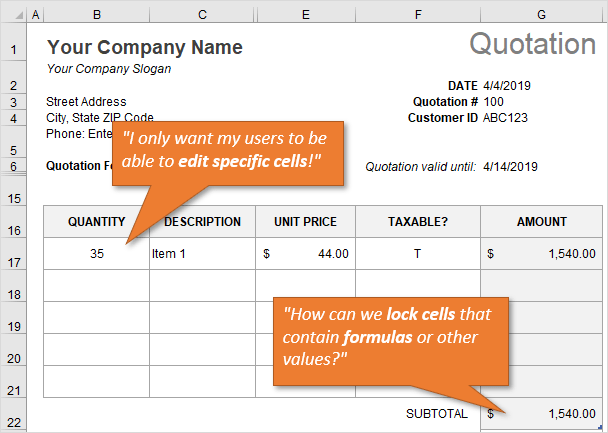
The great news is that you can lock or unlock any cell, or a whole range of cells, to keep your work protected. It’s easy to do, and it involves two basic steps:
- Locking/unlocking the cells.
- Protecting the worksheet.
Here’s how to prevent users from changing some cells.
Step 1: Lock and Unlock Specific Cells or Ranges
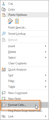
Right-click on the cell or range you want to change, and choose Format Cells from the menu that appears.
This will bring up the Format Cells window (keyboard shortcut for this window is Ctrl + 1.). Choose the tab that says Protection.
Next, make sure that the Locked option is checked.
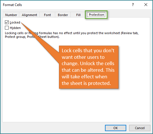
Locked is the default setting for all cells in a new worksheet/workbook.
Once we protect the worksheet (in the next step) those locked cells will not be able to be altered by users.
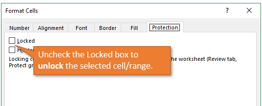
If you want users to be able to edit a particular cell or range, uncheck the Locked box so they are unlocked. Since cells are locked by default, most of the job will be going through the sheet and unlocking cells that can be edited by users.
I share some shortcuts to make this process faster in the Bonus section below.
Step 2: Protect the Worksheet
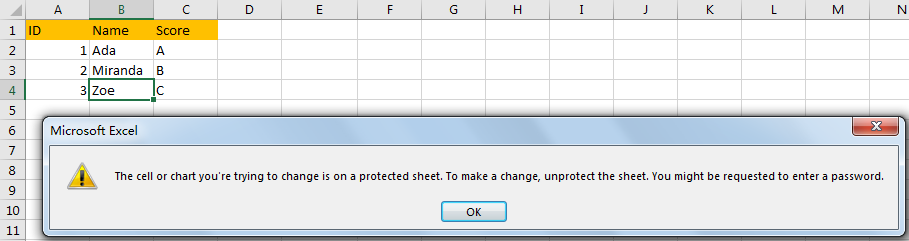
Now that you’ve locked/unlocked the cells that you want users to be able to edit, you want to protect the sheet. Once you protect the sheet, users cannot change the locked cells. However, they can still modify the unlocked cells.
To protect the sheet, simply right-click on the tab at the bottom of the sheet, and choose Protect Sheet… from the menu.
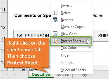
This will bring up the Protect Sheet window. If you want your sheet to be password protected, you have the option of entering a password here. Adding a password is optional. Click OK.
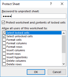
If you’ve chosen to enter a password, then you will be prompted to verify your entry after you’ve clicked OK.
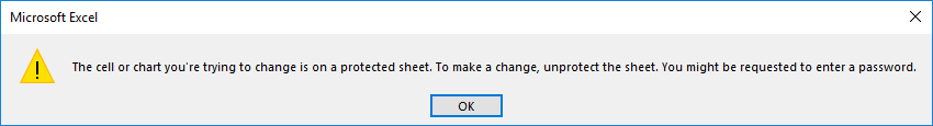
With the sheet protected, users will be unable to change the cells that are locked. If they try to make changes, they will get an error/warning message that looks like this.
You can unprotect the sheet in the same way that you protected it, by right-clicking on the sheet tab. An alternative way to protect and unprotect sheets is by using the Protect Sheet button in the Review tab of the Ribbon.
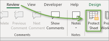
The button text displays the opposite of the current state. It says Protect Sheet when the sheet is unprotected, and Unprotect Sheet when it is protected.
It’s important to note that all cells can be edited when the sheet is unprotected. After making changes you must protect the sheet again and Save the workbook before sending or sharing with other users.
3 Bonus Tips for Locking Cells and Protecting Sheets
As you can see, it is fairly simple to protect your formulas and formatting from being changed! But I’d like to leave you with three tips to help make it faster & easier for both you and your users.
1. Prevent Locked Cells From Being Selected
This tip will help make it faster and easier for your users to input data in the sheet.
Turning off the Select locked cells option prevents the locked cells from being selected with either the mouse or keyboard (arrow or tab keys). This means users will only be able to select the unlocked cells that they need to edit. They can quickly hit the Tab, Enter, or arrow keys to move to the next editable cell.
To make this change, you just uncheck the option that says “Select locked cells” on the Protect Sheet window.
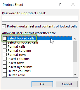
After pressing OK, you will only be able to select the unlocked cells.
2. Add a button for locking cells to the Quick Access Toolbar
This allows you to quickly see the locked setting for a cell or range.
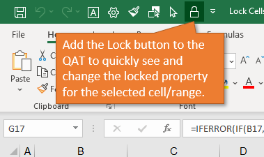
From the Home tab on the Ribbon, you can open the drop-down menu under the Format button and see the option to Lock Cell.
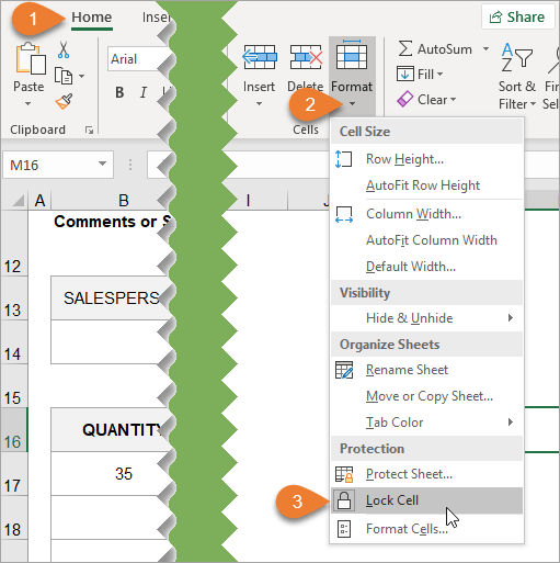
If you right-click on the Lock Cell option, another menu appears giving you the option to add the button to the Quick Access Toolbar.
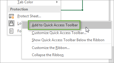
When you select this option, the button will be added to the Quick Access Toolbar at the top of the workbook. This button will remain each time you use Excel. You can easily lock and unlock specific cells on your sheet by clicking on this button.
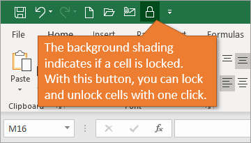
You can also see if the active cell locked or unlocked. The button will have a dark background if the selection is locked.
It’s important to note that this only shows the locked state of the active cell. If you have multiple cells selected, the active cell is the cell you selected first and appears with no fill shading.
Mixed Lock State
If you select a range that contains both locked and unlocked cells, you will see a solid box for the Locked checkbox in the Format Cells window. This denotes the mixed state.
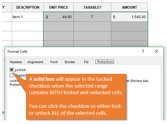
You can click the checkbox to lock or unlock ALL cells in the selected range.
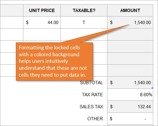
3. Use different formatting for locked cells
By changing the formatting of cells that are locked, you give your users a visual clue that those cells are off limits. In this example the locked cells have a gray fill color. The unlocked (editable) cells are white. You can also provide a guide on the sheet or instructions tab.
You might be wondering where I found this template for a quote. I got it from the template library. You can access the library by going to the File tab, choosing New, and using the search word “quote.”
You can find all sorts of useful templates there, including invoices, calendars, to-do lists, budgets, and more.
Conclusion
By locking your cells and protecting your sheet, you can keep your formulas safe from tampering by other users, and prevent mistakes.
I hope this simple tutorial proves helpful to you. Please leave a comment below if you have any tips or questions about locking cells, protecting sheets with passwords, or preventing users from changing cells.
Thank you! 🙂
What is Locking Cells in Excel?
In Excel, cells are locked to protect them from unwanted editing, deleting, and overwriting. Locking cells is specifically beneficial in cases where an excel worksheet needs to be shared with several colleagues.
For example, an organization Z provides consultation in taxation, audit, accountancy, insolvency, and other legal matters. Its finance director has asked Mr. A (subordinate in finance team) to create an Excel worksheet, which consists of:
- Market share captured by Z and its competitors over the past five years
- Deviations of the actual performance from the forecasts of the current year
- Sales revenueSales revenue refers to the income generated by any business entity by selling its goods or providing its services during the normal course of its operations. It is reported annually, quarterly or monthly as the case may be in the business entity’s income statement/profit & loss account.read more figures generated by the sales team in the present year
- Sales projections of the next two years
Further, Mr. A has been asked to share the worksheet with the marketing department to assist it in revising plans. For such inter-departmental collaboration, Mr. A wants his Excel data to be untouched as it circulates. This is where the cell locking property of Excel is used.
When working on shared files, the chances of making accidental changes to the data increase. Moreover, even slight modifications to the Excel formulas can lead to entirely different and erroneous results.
For addressing such issues, Excel provides a lock feature, which is always enabled by default. To confirm that the excel cells are locked, perform the following steps:
- Right-click on a cell and select “format cells.”
- Click the “protection” tab in the “format cells” window.
- The checkbox for “locked” is already selected, implying that the cells are locked.
Table of contents
- What is Locking Cells in Excel?
- Lock & Protect Protection of Formula Cells
- How to Lock Cells in Excel?
- Example #1–Lock Only the Excel Formula Cell
- Example #2–Lock Only the Final Excel Formula Cell
- Example #3–Lock all the Excel Formula Cells
- Frequently Asked Questions
- Recommended Articles
Lock & Protect Protection of Formula Cells
Before sharing a worksheet, one may want to lock and protect the excel formula cells. This is done to prevent entering an alphabet, a number or space in these cells. Moreover, no one is authorized to delete these cells other than the worksheet creator.
A locked excel cell can be edited or overwritten unless it is protected. To protect only the formula cells, perform the following steps in the mentioned sequence:
- Unlock all cells of the worksheet since they are locked, by default.
- Lock the formula cell.
- Protect the formula cell by protecting the worksheet.
Note: Only locking or only protecting cells does not prevent them from being changed. To secure a cell, it must be locked first and then protected.
How to Lock Cells in Excel?
Let us learn how to lock cells in Excel with the help of the following examples.
You can download this Lock Cell Formulas Excel Template here – Lock Cell Formulas Excel Template
Example #1–Lock Only the Excel Formula Cell
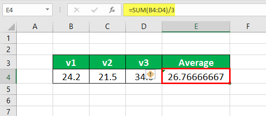
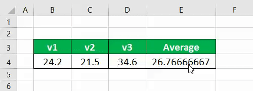
The following table shows three numeric values titled “v1,” “v2,” and “v3.” We want to calculate the average of these values.
Further, lock and protect the cell in excel, which displays the formula of average.
The steps to calculate the average and thereafter protect the formula cell are listed as follows:
Step 1: Enter the average formula in cell E4.
Step 2: Unlock the already locked cells of the excel tableIn excel, tables are a range with data in rows and columns, and they expand when new data is inserted in the range in any new row or column in the table. To use a table, click on the table and select the data range.read more. For this, select any cell within the table and press “Ctrl+A” (or Command+A) together.
Alternatively, unlock the entire worksheet by selecting any cell outside the table and pressing “Ctrl+A.” The subsequent steps 3 and 4 can also be applied for unlocking the worksheet.
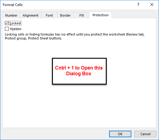
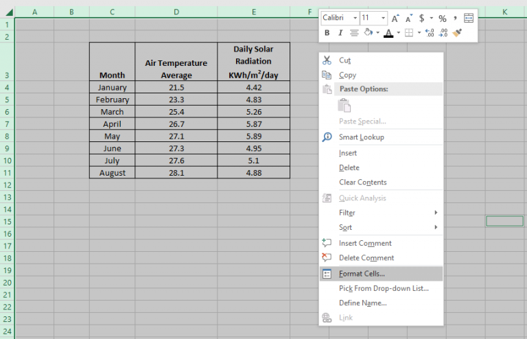
Step 3: Press “Ctrl+1” (or Command+1) together. The “format cells” dialog box appears, as shown in the following image.
Alternatively, right-click the selection and choose “format cells” from the context menu.
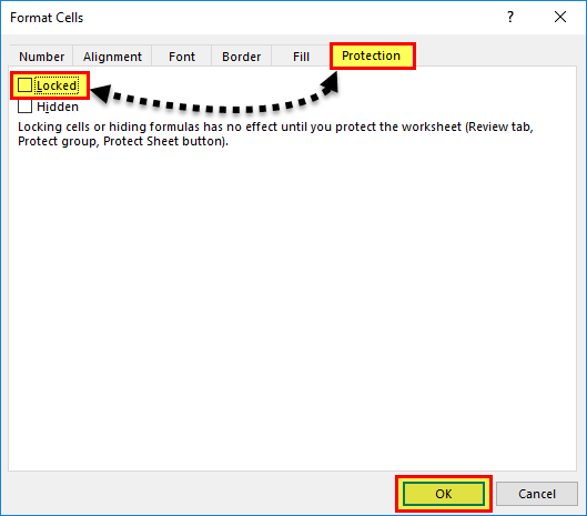
Step 4: In the “protection” tab, deselect the “locked” option. Click “Ok.”
Step 5: All the cells of the table are unlocked.
Step 6: Select the cell containing the formula (E4). Perform the following steps in the mentioned sequence:
- Press “Ctrl+1” together.
- The “format cells” dialog box opens.
- In the “protection” tab, select the “locked” option, as shown in the following image.
- Click “Ok.”
The formula cell E4 is locked.
Step 7: Protect the formula cell by clicking “protect sheet” in the Review tab.
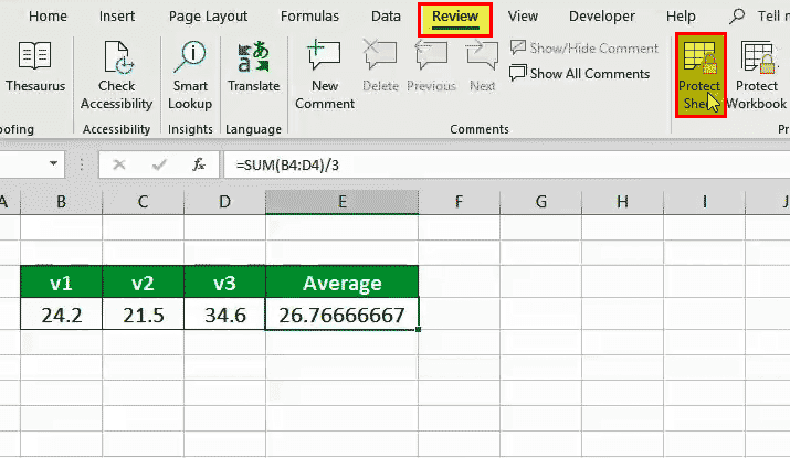
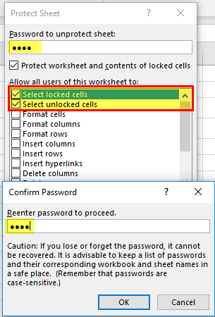
Step 8: Enter a password and click “Ok.” Confirm the password and click “Ok” again.
Note: It is optional to enter a password. In case a password is not provided, anyone using the Excel worksheet can unprotect the sheet and change its content.
Step 9: The formula cell is locked and protected in excel. If you try to edit the cell E4, a message appears stating that the cell is protected.
The same is shown in the following image.
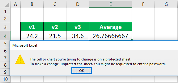
Only the formula cell E4 is protected. If you try to overwrite any other cell of the given table, no message is displayed. This is because the remaining cells of the table are not protected.
Note: Only the locked cells in Excel can be protected.
Example #2–Lock Only the Final Excel Formula Cell
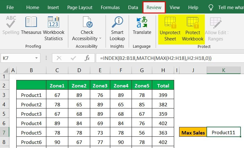
The following table shows the zone-wise sales (in $) of 16 different products. We want to calculate the total sales of each product.
Further, lock and protect the cell in excel which displays the highest sales of a product. The cells containing sales and total product sales should remain editable.
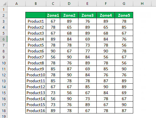
The steps to calculate the total product sales and thereafter protect the final formula cell are listed as follows:
Step 1: Enter the following formula in cell H3 to calculate the total sales of each product.
“=SUM(C3:G3)”
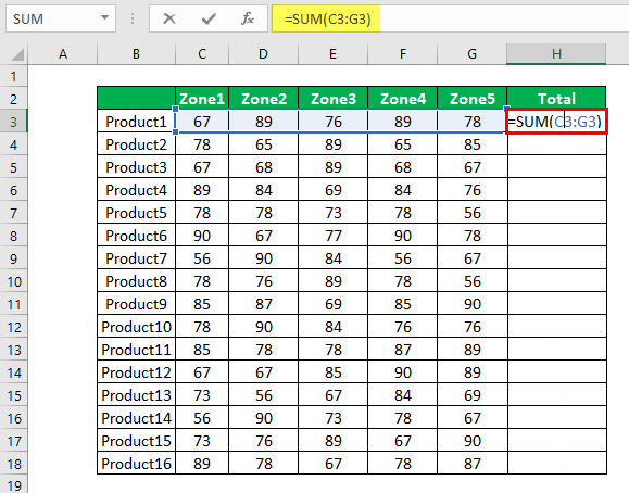
Step 2: Press the “Enter” key and drag the formula to the remaining cells, as shown in the following image.
Note: A green triangle appearing on top of the cells of column H (range H3:H18) indicates that the formulas are unlocked.

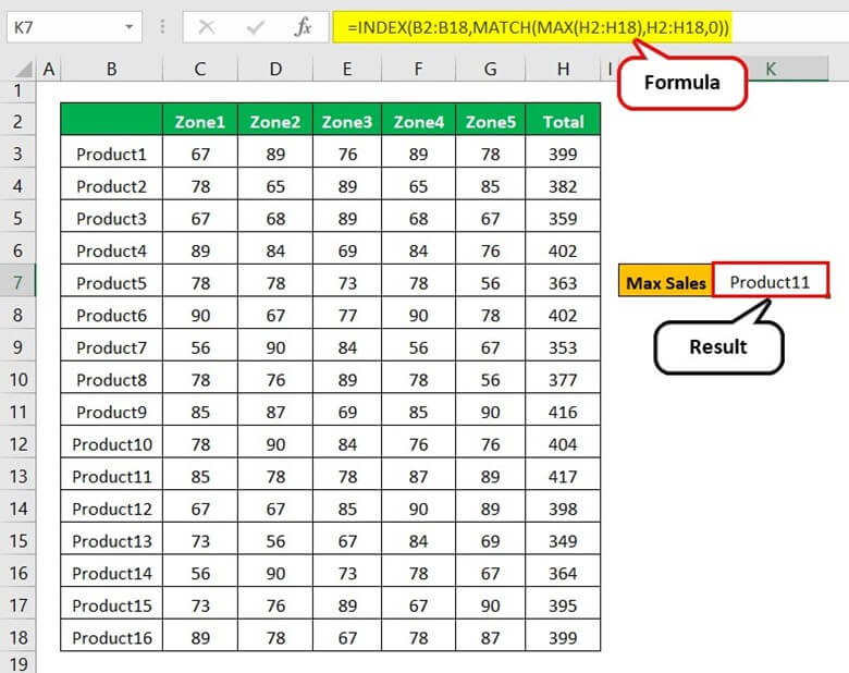
Step 3: Enter the following formula in cell K7 to identify the product with the highest sales.
“=INDEX(B2:B18,MATCH(MAX(H2:H18),H2:H18,0))”

Step 4: Press the “Enter” key. The product with the highest sales appears in cell K7.
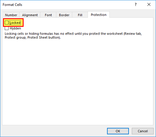
Step 5: To protect only the formula cell K7, unlock all the cells of the worksheet in the mentioned sequence:
- Press the keys “Ctrl+A” together. This selects all the cells of the worksheet.
- Press the keys “Ctrl+1” together. This opens the “format cells” dialog box.
- In the “protection” tab, deselect the “locked” option.
- Click “Ok.”
All the cells of the worksheet are unlocked.
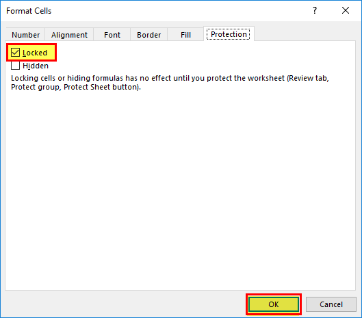
Step 6: To lock cell K7, perform the following steps in the mentioned sequence:
- Select the cell K7 containing the formula.
- Press “Ctrl+1” together.
- In the “format cells” dialog box, select the “locked” option under the “protection” tab.
- Click “Ok.”
The formula cell K7 is locked in excel.
Step 7: To protect cell K7, perform the following steps in the mentioned sequence:
- In the Review tab, click “protect sheet.”
- Enter a password and click “Ok.”
- Confirm the password and click “Ok.”
Hence, the formula cell K7 is locked and protected. The remaining cells containing sales (columns C to G) and total product sales (column H) are editable.
Note: Once a sheet is protected, the “unprotect sheetOnce the workbook has been password-protected, one must input the exact password that was entered while protecting the workbook in order to unprotect it.read more” option appears in the Review tab, as shown in the following image.
Example #3–Lock all the Excel Formula Cells
Let us understand the protection of Excel formulasProtect Excel Formulas are the critical element of Excel files to create reports or organize the data, without which one cannot modify or make changes at any time.read more with the help of the “go to special” feature.
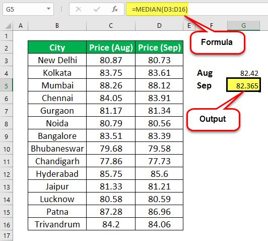
The following table shows the oil prices of different cities for August and September 2018. We want to calculate the median prices for the given months. In addition, identify the month with the higher median price.
Further, lock all the cells which contain formulas by using the “go to special” feature.
The steps to calculate the median prices and thereafter protect all the formula cells are listed as follows:
Step 1: Enter the following formula in cell G4 to calculate the median prices for August.
“=MEDIAN(C3:C16)”
Press the “Enter” key and the output appears in cell G4.

Step 2: Enter the following formula in cell G5 to calculate the median prices for September.
“=MEDIAN(D3:D16)”
Press the “Enter” key and the output appears in cell G5.
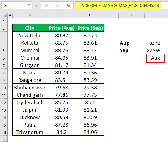
Step 3: Enter the following formula in cell G6 to identify the month with the higher median price.
“=INDEX(F4:F5,MATCH(MAX(G4:G5),G4:G5,0))”
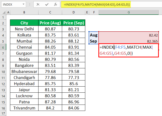
Step 4: Press the “Enter” key. The month with the higher median price appears in cell G6.
Step 5: To protect the cells containing the formula, unlock all the cells in Excel. For this, perform the following steps in the mentioned sequence:
- Select all the cells of the worksheet by pressing “Ctrl+A” together.
- Press “Ctrl+1” together and the “format cells” dialog box opens.
- In the “protection” tab, deselect the “locked” option.
- Click “Ok.”
All the cells of the worksheet are unlocked.

Step 6: In the Home tab, click the “find and select” drop-down in the “editing” group. Select the “go to special” option, as shown in the following image.
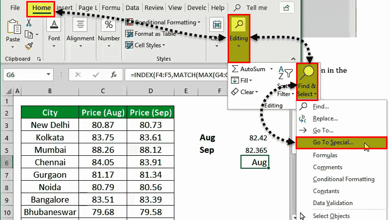
If you are using Mac, select “go to” in the Edit tab. Click “special.”
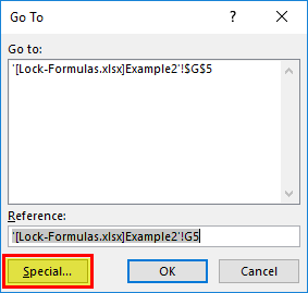
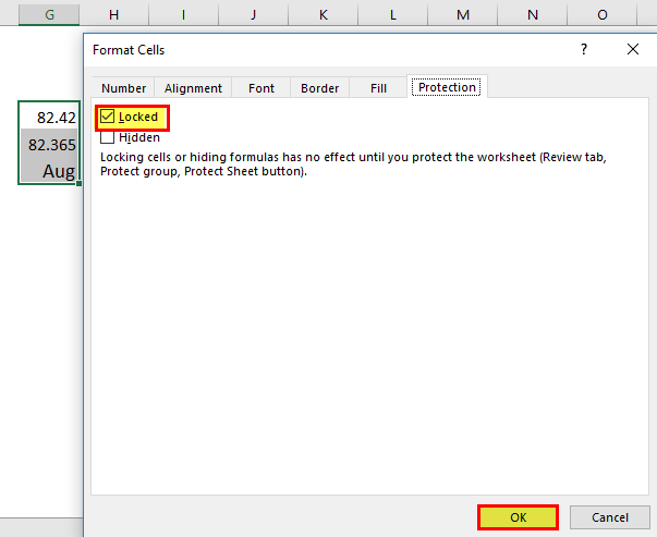
Step 7: The “go to special” dialog box opens. Select “formulas” and click “Ok.”

Step 8: All the cells containing the formulas (G4, G5, and G6) are selected. To lock these excel cells, perform the following steps in the mentioned sequence:
- Press the keys “Ctrl+1” together.
- The “format cells” dialog box appears, as shown in the following image.
- In the “protection” tab, select the “locked” option.
- Click “Ok.”
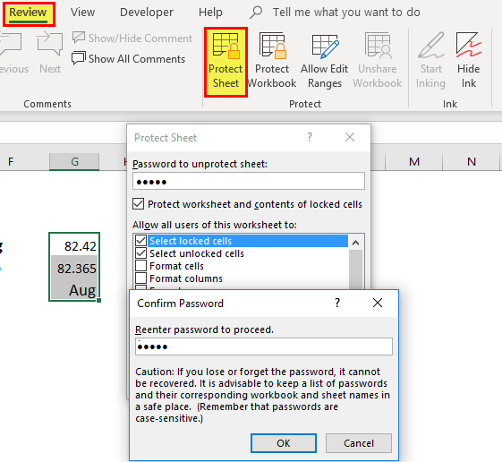
Step 9: To protect the formula cells, perform the following steps in the mentioned sequence:
- Click “protect sheet” under the Review tab.
- Enter a password (optional) and click “Ok.”
- Re-enter the password to confirm it.
- Click “Ok.”
All the formulas cells (G4, G5, and G6) are now protected.
Frequently Asked Questions
1. What does it mean to lock cells in Excel and how is it done?
Locking excel cells is a technique of protecting them from changes like editing, deleting, and overwriting. It is possible to lock and unlock either a part or the entire worksheet.
For instance, it is possible to lock specific cells and leave the remaining data unlocked. Likewise, the user can edit the raw data (input cells), but the formula cells that calculate the output can be locked.
By default, the worksheet is locked. To lock or unlock the entire excel worksheet, the steps are listed as follows:
a. Select the entire worksheet by pressing “Ctrl+A.”
b. Right-click the selection and choose “format cells” from the context menu.
c. Select the “locked” option to lock all cells. Alternatively, uncheck the “locked” option to unlock all cells.
d. Click “Ok.”
All cells of the worksheet are locked or unlocked depending on the action performed in “step c.”
2. How to lock and protect specific cells in Excel?
The steps to lock and protect specific cells in Excel are listed as follows:
a. Unlock all cells of the excel worksheet
• Select the entire worksheet by pressing “Ctrl+A.”
• Right-click the selection and choose “format cells” from the context menu. Alternatively, press “Ctrl+Shift+F” or “Ctrl+1.”
• In the “format cells” dialog box, uncheck the “locked” option. Click “Ok.”
b. Select the cells or ranges to be locked.
• For adjacent cells–select the cells to be locked with the help of “Shift” and the arrow keys.
• For non-adjacent cells–select the cells to be locked by pressing and holding the “Ctrl” key.
c. Lock the selected cells
• Press “Ctrl+1” together and the “format cells” dialog box opens.
• Select the “locked” option in the “protection” tab. Click “Ok.”
d. Protect the worksheet
• Click “protect sheet” in the “changes” group of the Review tab. Alternatively, right-click the sheet name appearing at the bottom left-hand side. Select “protect sheet” from the context menu.
• Enter a password which is optional and click “Ok.”
• Confirm the password and click “Ok.”
The specific cells are locked and protected while the remaining cells are editable.
Note: While entering the password, you can select the actions that the users are allowed to perform.
3. How to lock multiple cells and protect them without using a password in Excel?
For locking multiple cells, an important point to consider is the selection of cells. It is possible to select a range of cells which can be either adjacent or non-adjacent. The selection of ranges is carried out as follows:
• For an adjacent range: Select by using the “Shift” and arrow keys together.
• For a non-adjacent range: Select by pressing and holding the “Ctrl” key.
• For one column: Select any cell within the column to be locked and press “Ctrl+Space.”
• For multiple non-adjacent rows or columns: Click the different row or column labels (on the left or on top) by pressing and holding the “Ctrl” key.
Once the cells are selected, they can be locked and protected. This is done by pressing “Ctrl+1” and selecting the “locked” option in the “protection” tab. Further, click “protect sheet” under the Review tab.
Cells can be protected without supplying a password as well. For this, just omit supplying the password while protecting a sheet in the Review tab.
However, one must remember that if a password is not provided, the worksheet content can be changed by anyone. This is because the “unprotect sheet” option can be availed by any user.
Recommended Articles
This has been a guide to lock cells in Excel. Here we discuss how to lock excel formula cells in Excel, along with practical examples and downloadable Excel templates. For more on Excel, take a look at the following articles–
- Checkbox in ExcelA checkbox in excel is a square box used for presenting options (or choices) to the user to choose from.read more
- Scroll Lock in ExcelWhen we press the down arrow key from any cell, it normally moves us to the next cell below it, but when we have scroll lock turned on, it drags the worksheet down while the cursor stays in the same cell.read more
- Last Day of the Month in ExcelThe EOMONTH function can be used to find the last day of the month. This function’s functionality is not limited to knowing the current month’s last day; we may also choose to know the previous and next month’s last days.read more
Many users used to lock cells in Excel so that no one can modify the content of the protected cells without their permission. Thus, if you also want to restrict someone from making changes to your Excel cells then read this blog. This post contains different ways to lock Excel cells and make them protected.
Quick Ways |
Step-By-Step Solutions Guide |
|
Way 1- Lock Cells In Excel Worksheet |
Choose the cells >> go to the Home tab and then from the Alignment…Complete Steps |
|
Way 2- Lock Some Specific Cells In Excel |
Choose the entire worksheet >> go to Home tab >> hit sign of the dialog box launcher…Complete Steps |
|
Way 3- Lock Excel Cells Using VBA Code |
Choose entire cells in Excel spreadsheet >> go to the Home tab >> cells >> Format…Complete Steps |
|
Way 4- Protect Entire Worksheet Except Few Cells |
Press Control + 1 key >> in the opened Format Cells dialog box >> go to ‘Protection’...Complete Steps |
|
Way 5- Lock Formula Cells |
Choose Format Cells >> go to Protection tab >> untick Locked option >> OK…Complete Steps |
To repair & recover corrupted Excel file data, we recommend this tool:
This software will prevent Excel workbook data such as BI data, financial reports & other analytical information from corruption and data loss. With this software you can rebuild corrupt Excel files and restore every single visual representation & dataset to its original, intact state in 3 easy steps:
- Download Excel File Repair Tool rated Excellent by Softpedia, Softonic & CNET.
- Select the corrupt Excel file (XLS, XLSX) & click Repair to initiate the repair process.
- Preview the repaired files and click Save File to save the files at desired location.
What’s The Need To Lock Cells In Excel?
The plus point of locking cells in Excel is that it protects your data from the unwanted changes.
Suppose you have to share your Excel spreadsheet with other users and there are some specific cells which you don’t want to get modified. In that case, cell lock is the best trick to avoid formula and formatting changes like issues.
Way 1- Lock Cells In Excel Worksheet
Follow the below-mentioned solutions to do so:
- Choose the cells which you need to lock.
- Go to the Home tab and then from the Alignment group tap to the small arrow present across it. This will open the windows of Format Cells.
- Now in the format cell window go to the Protection tab and choose the check box of Locked After that tap to the OK button to shut off this popup window.

Note: If you are attempting these steps on the worksheet or workbook which you haven’t protected then you will find that the cells are locked already. This implies that the cell can also be locked when the workbook or worksheet is protected.
- From the excel ribbon hit the Review After that from the Changes group, you have to choose either the Protect Workbook or Protect Sheet.
- Next, you have to reapply the protection over your workbook or worksheet.
Tip: well it’s a best solution to unlock cells which you need to modify before protecting a workbook or worksheet. But don’t get worried as you can unlock them easily even after applying protection over it. For removing up the protection, all you need to do is just remove the applied password.
Also Read: 5 Tricks To Protect Excel Workbook From Editing
Way 2- Lock Some Specific Cells In Excel
Sometimes you just need to lock some individual cells which contain important data or formulas. In such cases, only protect the cells which you need to lock leaving the rest one as it is.
By default, entire cells are comes locked, so if you apply protection to your sheet then entire cells are also get locked.
So, make sure that only those cells are protected which you want to lock and after that only apply protection to the whole worksheet.
Follow the steps to lock some specific cells in Excel
- Choose entire worksheet and then go to the Home tab.
- After that hit, the sign of the dialog box launcher presents the alignment group.
- Now in the opened dialog box of Format Cells, got to the Protection tab and uncheck the Locked option. Hit the OK button.
- Choose the cells which you need to lock.
- Again make a tap over the dialog box launcher present in the Alignment group which is under the Home tab.
- Now again in the opened dialog box of Format Cells go to the Protection tab and make a check mark across the Locked option.
- Doing this will unlock entire cells of your worksheet except the one which you have selected for locking.
- Now go to the Review tab and then from the Changes group hit the Protect Sheet option.
- From the opened dialogue box of Protect Sheet:
- Check whether the option of ‘Protect worksheet and contents of locked cells’ is checked or not. If it’s not then check it.

- Enter the password to apply password on your sheet.

- Now specify the permission which you want to assign to other users. By default, you will see that the first two options are already selected. Using which user can easily make selection for the locked or unlocked cells.
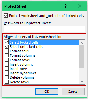
- Apart from this you can also allow other options like inserting rows/columns or making changes in the formatting.
- Tap to the OK button.

If you are applying any password then you are asked to reconfirm it.
When the next time you try to edit those specific cells, you will get the following error message pop-up dialog box.
Way 3- Lock Excel Cells Using VBA Code
- Choose entire cells in your Excel spreadsheet.
- Now go to the Home tab first and then to cells from this cell section tap on the Format option and choose the format cells option.
- This will open a Format Cells dialogue box. On this opened dialog box, you need hit the Protection tab. Here you have un-select the option Locked.

- Now in your Excel file where name of your sheet appears. Make a right click from your mouse and choose the View Code.
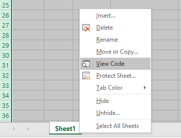
- This will open Microsoft Visual Basic for Applications dialogue box. In this opened white sheet along with the dialogue box, you just need to type the below code.
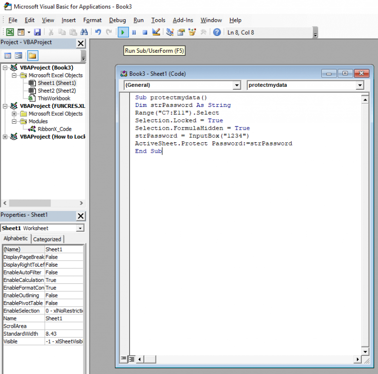
- In the written code, we have selected the data range from C7 to E11. And have also applied a password like, 1234.
- After entering the complete code go to the Debug Here you will find a Run Sub/User Form (F5) option tap on it.
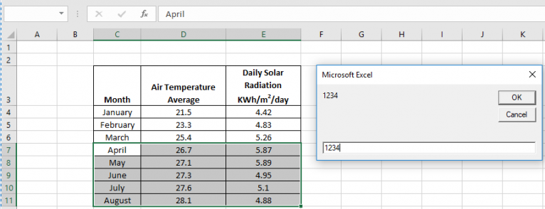
- Now you will see that your Excel worksheet is opening along with a password window.
- So, write same password that you as allotted in the VBA code eg: 1234.
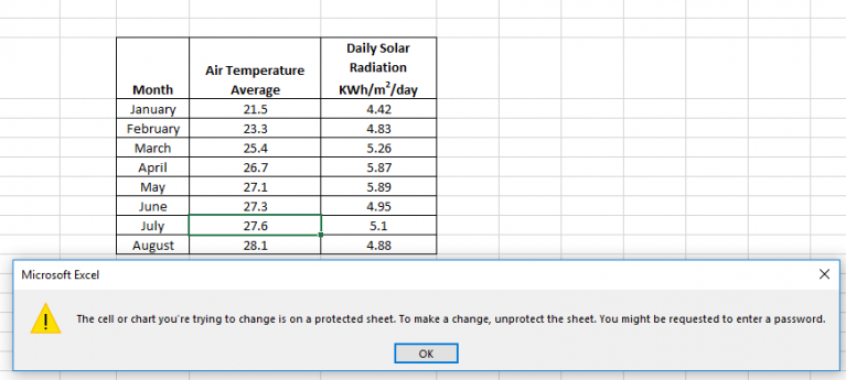
- After doing this whenever you approach for making changes in the desired cells of the Excel. This will throw a warning message stating that “you can’t edit the cells as it is protected”.
Note: To unlock the cells locked with Excel VBA code you have to follow the same unlocking procedures as explained earlier.
Also Read; Top 3 Methods To Unlock Password Protected Excel File
Way 4- Protect Entire Worksheet Except Few Cells
In some cases, people also want to protect the entire worksheet by keeping some of the cells unlocked.
Well, such a situation arises when you have added interactive features in your worksheet like a drop-down list. And you want that your drop-down keeps working even when the worksheet is protected.
To accomplish this task, just follow the below-mentioned steps:
- Make a selection of the cells which you want to keep unlocked.
- Press the Control + 1 key from your keyboard.
- In the opened Format Cells dialog box go to the ‘Protection’.
- Unselect the Locked option and hit the OK button.
Now if the entire worksheet is kept protected, these particular cells should work normally.
For this you have to perform the following steps, so as to protect the entire worksheet except the selected cells:
- Hit the Review tab and then from the Changes group tap to the Protect Sheet icon.
- In the opened Protect Sheet dialog box:
- Check whether the option of ‘Protect worksheet and contents of locked cells’ is checked or not. If it’s not then check it.

- Enter the password to apply password on your sheet).
- Now specify the permission which you want to assign to other users. By default, you will see that the first two options are already selected. Using which user can easily make selection for the locked or unlocked cells.
- Apart from this you can also allow other options like inserting rows/columns or making changes in the formatting.

Way 5- Lock Formula Cells
To lock formula cells, the very first thing you need to do is unlock all the cells and then only lock the cells having the formula in it. At last protect the sheet.
Well if you don’t know how to perform all these tasks then follow the below steps:
- Choose entire cell of your worksheet.

- Now make a right click and from the listed option choose the Format Cells.
- On the opened format cell window go to the Protection tab and untick the check box of Locked option. After that hit the OK button.

- Go to the Home tab and then from the Editing group choose the Find & Select.

- Hit the Go To Special option.

- Choose Formulas and hit the OK button.
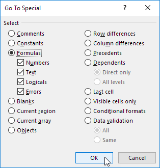
You will see that after doing these steps Excel will selects all the formula cells.

- Press the CTRL + 1 button from your keyboard.
- Go to the Protection tab and select the check box of Locked option. After that press the OK button.
Note:
If you select the check box of Hidden option then the user will not be able to see the formula within the formula bar even after choosing the formula cells.
Always keep in mind that locking cells doesn’t have any effect until and unless the worksheet is protected.
- So now it’s time to protect your Excel sheet.
After this, you will see that entire the formula cells are been locked. In case of editing these cells, firstly you need to unprotect the worksheet.
Use Excel Repair Tool to Repair/Recover Corrupted Excel Documents
MS Excel Repair Tool is a special tool that is specifically designed to repair any sort of issues, corruption, errors in Excel file. This can also easily restore entire lost Excel data including cell comments, charts, worksheet properties, and other related data.
It is a unique tool that can repair multiple corrupted Excel files in one repair cycle and restore data to a new blank Excel file or the preferred location. The tool has the ability to recover data without modifying the original formatting.
- The interface is very simple, with a large toolbar of buttons to add files or folders to the application.
- With this software, you can repair your corrupted Excel file.
- It can easily restore all corrupt excel files and also recover everything which includes cell comments, charts, worksheet properties, and other related data.
- The corrupted excel file can be restored to a new blank Excel file.
- It has the ability to recover the complete Excel file data from the file and restore them even without modifying the original formatting.
* Free version of the product only previews recoverable data.
Steps to Utilize MS Excel Repair Tool:
Related FAQs:
Can I Lock Multiple Cells in Excel?
Yes, you can lock multiple cells in Excel through freeze panes. Apart from that, you can use a shortcut key- F4 to lock specific columns or rows in the document as well as the range of cells that you want to lock.
How Do I Make a Cell Non-Editable in Excel?
To make a cell non editable in Excel, you need to make cell as read only using VBA code. Although using the VBA code helps to make cell as read-only so that no one can edit them and even you don’t have to lock the cells to protect your worksheet data.
Does F4 Lock Cells in Excel?
Yes, the F4 key is a shortcut mode or we can say the easiest way to lock cells in the MS Excel.
Bottom Line
Locking cells in Excel help you to keep the formula completely safe from being tempered by any third-party user.
Hopefully, this informative tutorial seems helpful to you on how to protect cells in excel without protecting sheets. Don’t forget to leave a comment if you have any queries or tips to share about how to lock cells in Excel and protect them.


Priyanka is an entrepreneur & content marketing expert. She writes tech blogs and has expertise in MS Office, Excel, and other tech subjects. Her distinctive art of presenting tech information in the easy-to-understand language is very impressive. When not writing, she loves unplanned travels.