Lock rows in excel

Freeze panes to lock rows and columns

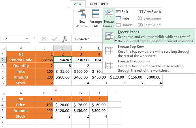
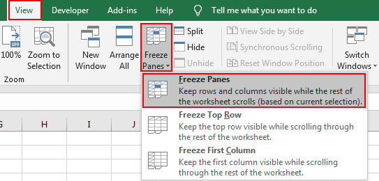
To keep an area of a worksheet visible while you scroll to another area of the worksheet, go to the View tab, where you can Freeze Panes to lock specific rows and columns in place, or you can Split panes to create separate windows of the same worksheet.

Freeze rows or columns

Freeze the first column

• Select View > Freeze Panes > Freeze First Column.

            The faint line that appears between Column A and B shows that the first column is frozen.

Freeze the first two columns

1. Select the third column.

2. Select View > Freeze Panes > Freeze Panes.

Freeze columns and rows

1. Select the cell below the rows and to the right of the columns you want to keep visible when you scroll.

2. Select View > Freeze Panes > Freeze Panes.

Unfreeze rows or columns

• On the View tab > Window > Unfreeze Panes.

  

  Note: If you don’t see the View tab, it’s likely that you are using Excel Starter. Not all features are supported in Excel Starter.

Need more help?

You can always ask an expert in the Excel Tech Community or get support in the Answers community.

See Also

Freeze panes to lock the first row or column in Excel 2016 for Mac

Split panes to lock rows or columns in separate worksheet areas

Overview of formulas in Excel

How to avoid broken formulas

Find and correct errors in formulas

Keyboard shortcuts in Excel

Excel functions (alphabetical)

Excel functions (by category)

The Microsoft Excel program is designed not only to enter data into the table conveniently and edit it as you need it, but also to view large blocks of information. Most people using PCs work with it constantly.

The columns and rows names can be significantly removed from the cells with which the user is working at this time. Scrolling the page to see the name of the document is not comfortable for any user. Therefore, the Tabular Processor has possibilities to fix certain areas.



Locking a row in Excel while scrolling

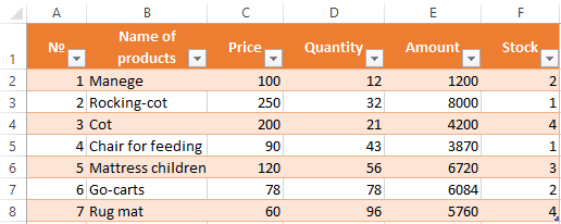
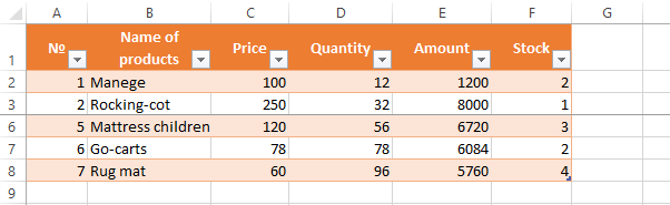
Usually an Excel table has one cap. Meanwhile, this document can have up to thousands of rows. Working with multipage table blocks is inconvenient when column names are not visible. Scrolling the page to its beginning to return to the correct cell is absolutely irrational. To make the cap visible when scrolling, fix the top row of the Excel table, following these actions:

1. Create the needed table and fill it with the data.



2. Make any of the cells active. Go to the “VIEW” tab using the tool “Freeze Panes”.



3. In the menu select the “Freeze Top Row” functions.

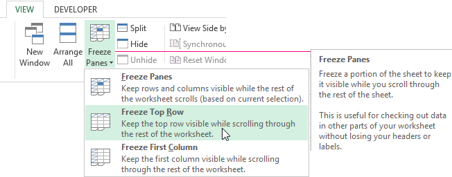
You will get a delimiting line under the top line. Now when you scroll vertically the table cap will be always visible.



Locking several rows in Excel while scrolling

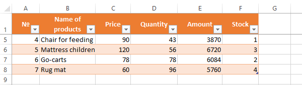
Let us suppose, a user needs to fix not only the cap. For instance, another row or even a couple of rows must be fixed when scrolling the document. Doing it is possible and easy, when you follow these steps:

1. Select any cell under the line, which we will fix. This action will help Excel to “understand”, which area should be fixed;
2. Now select the “Freeze Panes” tool.

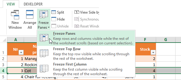
When you perform horizontal and vertical scrolling, the cap and the top row of the table remain fixed. Thus, you can fix two, three, four and more rows.

Note: This method works for 2007 and 2010 Excel versions. In earlier versions the “Lock areas” tool is located in the “Window” menu on the main page. There you must always (!) activate the cell under the freeze row.

Freezing columns in Excel

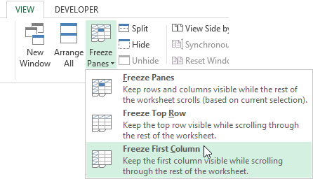
For instance, the information in the table has a horizontal direction. It is not concentrated in columns, but located in rows. For his comfort, the user must freeze the first column, containing the lines’ names in horizontal scrolling.

1. Select any cell of the chosen table so that Excel understands with what data it will work. Pin the first column in the menu you will see..



2. Now, when the document is scrolled to the right horizontally, the needed column will be fixed.

To freeze several columns, select the cell at the page bottom (to the right from the fixed column). Pick the “Freeze Panes” button.

How to freeze the row and column in Excel

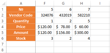
You have a task – to freeze the selected area, which contains two columns and two rows.

Make a cell at the intersection of the fixed rows and columns active. However, the cell must be not placed in the fixed area. It should have the position right under the required lines (to the right of the required columns). Pick the first option in Excel Locking Areas. The photo shows that when scrolling, the selected areas remain at the same place.

Removing a fixed area in Excel

After fixing a row or a column of the table the button deleting all pivot tables becomes available.

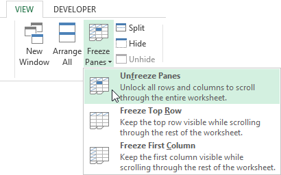
After clicking – «Unfreeze Panes», all the locked areas of the worksheet become unlocked.

(Note: This guide on how to lock a row in Excel is suitable for all Excel versions including Office 365)

When working with data, Excel can be an invaluable tool to help you organize, analyze, and visualize data. But imagine if you’re working on a large spreadsheet and you don’t want certain rows to move when you scroll. No need to stress as Excel allows you to lock a row in place so that it remains visible as you scroll down or to the side. 

If you don’t know how to do it, worry not! In this article, I will tell you how to lock a row in Excel in 4 proven useful ways. 

You’ll learn:

• What Is a Locked Row?
• How to Lock a Row in Excel?
• By Using Freeze Panes
• By Using Protect Sheet
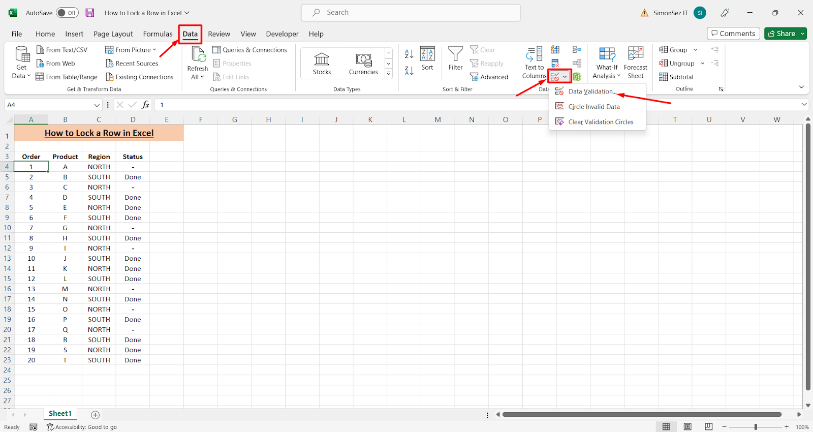
• By Using data Validation
• By Using Conditional Formatting
• How to Lock a Row in Excel in 7 Simple Steps?
• Benefits of Locking Rows in Excel

Related Reads

HOW TO DELETE ROWS IN EXCEL? 6 EFFICIENT WAYS

HOW TO CHANGE ROW HEIGHT IN EXCEL? 5 EASY WAYS

HOW TO FREEZE ROWS IN EXCEL? 4 EASY STEPS

What Is a Locked Row?

Before moving on to see how to lock a row in Excel, let us first understand what a locked row is.

A locked row in Excel is a row that is protected from changes. This means that any changes you make to the sheet will not affect the locked row, and you will not be able to delete, insert, or move it. 

Locking rows in Excel allows you to protect critical information and maintain the integrity of your data. While there’s no limit to the number of rows you can lock in Excel, it’s important to note that locked rows are only effective when the entire sheet or workbook is protected.

Once you lock a row, Excel adds a lock symbol to the upper-left corner of the row. You can also tell if a row is locked by looking for a thin line at the top of the row.

Sometimes, Excel may prevent you from locking a row in certain circumstances. For example, if you’re trying to lock the header row of a table, Excel won’t allow it. This is because the header row is usually used to identify the columns in a worksheet, and locking it would prevent you from being able to make changes to the table.

Another example can be found when working with an Excel spreadsheet that contains formulas. If you try to lock a row that has a formula in it, Excel won’t let you. This is because the formulas rely on data in other cells, and locking the row would prevent the formula from accessing the necessary data.

How to Lock a Row in Excel?

There are several ways to lock a row in Excel:

By Using Freeze Panes

Freeze panes allow you to lock certain rows and columns in place so that when you scroll down or across the worksheet, the locked rows and columns remain visible. 

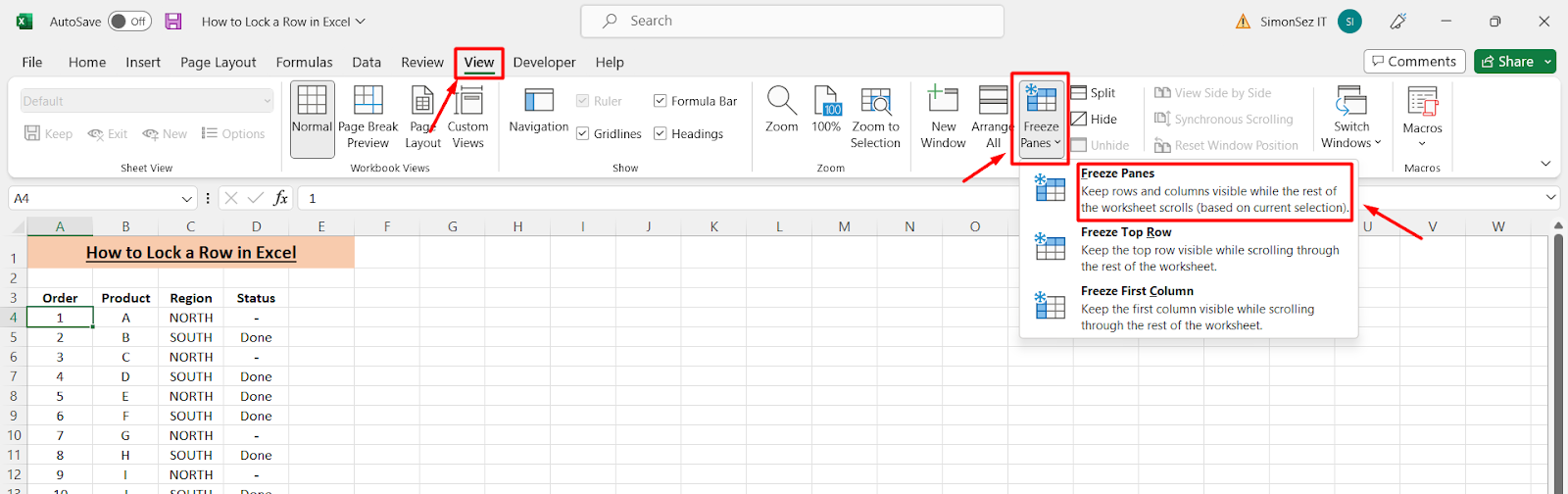
• To do this, select the row below the row you want to lock, then go to View. Click on the dropdown from Freeze Panes and select Freeze Panes. This will lock all rows above the row you selected.

By Using Protect Sheet

You can also lock a row in Excel by using the Protect Sheet feature. The Protect Sheet feature in Excel is a security feature that enables users to lock certain parts of a worksheet, such as cells, ranges, objects, or sheets. 

Using the Protect Sheet feature, you can prevent other users from making changes to the data or formatting a specific worksheet. It also allows you to set permissions for other users, so they can view and edit specific parts of the worksheet.

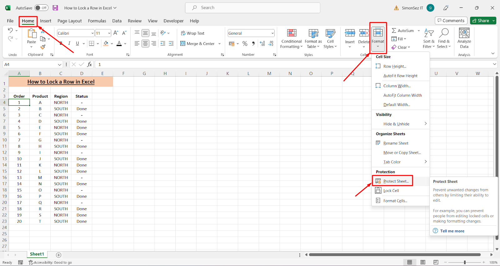
• To do this, go to Home. Click on the dropdown from Format and click on Protect Sheet. Select the Locked checkbox next to the rows you want to lock. You can also select the Hidden checkbox to hide the locked rows.

By Using data Validation

Data validation is a feature in Excel that allows you to restrict values that can be entered into a cell. 

• To lock a row in Excel using data validation, select the row you want to lock, then go to Data. Click on the dropdown from Data Validation. Select the Allow only list and enter the values you want to allow. This will lock the row so that no other values can be entered.

By Using Conditional Formatting

Conditional formatting is a feature in Excel that allows you to set rules for when a cell should be formatted based on the value in the cell.

• To lock a row in Excel using conditional formatting, select the row you want to lock, then go to Home. Click on the dropdown from Conditional Formatting and click on New Rule. Select the Format-only cells that contain the option and enter the values you want to allow. This will lock the row so that no other values can be entered.

Now the question is how to lock a row in Excel, the easy way.

Suggested Reads

HOW TO MOVE ROWS IN EXCEL? 5 EASY METHODS

HOW TO USE THE EXCEL COLLAPSE ROWS FEATURE? — 4 EASY STEPS

ARROW KEYS NOT WORKING IN EXCEL – 4 EASY FIXES

How to Lock a Row in Excel in 7 Simple Steps?

Suppose you are working on a spreadsheet in Excel and want to lock a certain row so that it cannot be edited or moved. Just follow these simple steps.

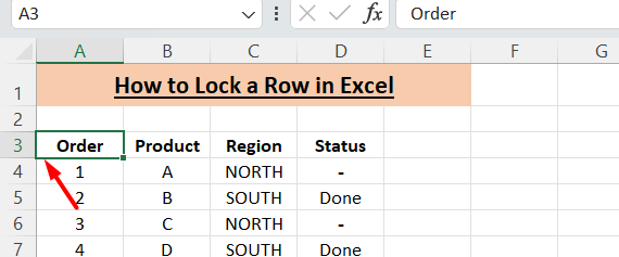
• Step 1. Select the row or rows you wish to lock. You can do this by clicking and dragging on the row headers. To select adjacent or non-adjacent rows, hold the keys Shift or Ctrl and select the individual rows respectively.

• Step 2. Right-click the selection and select “Format Cells” from the popup menu.

• Step 3. Select the “Protection” tab in the Format Cells dialog box.

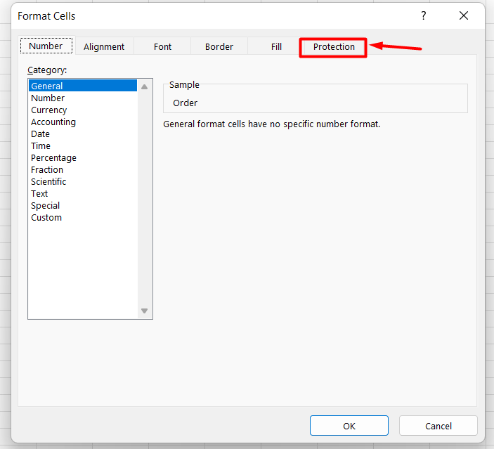
• Step 4. Check the “Locked” box and click “OK” to close the dialog box.

• Step 5. But if you want to protect the spreadsheet, go to the “Review” tab, click on “Protect Sheet,” and then enter a password if you want to.

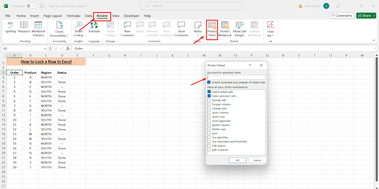
• Step 6. Click “OK,” and the selected row will be locked.

• Step 7. To unlock a row, follow the same steps, but uncheck the “Locked” box in the Format Cells dialog box.

Benefits of Locking Rows in Excel

Locking rows in Excel provides the following benefits:

1. Protect Data: Locking rows and columns in a spreadsheet can protect essential data from being accidentally deleted or changed. This is especially useful when you have formulas that rely on specific data in the spreadsheet.

Related Read: How to Password Protect an Excel File? 2 Effective Ways

1. Prevent Accidental Editing: It’s very easy for users to accidentally delete or modify data in a spreadsheet. Locking rows and columns can help prevent accidental editing from happening.

1. Ensure Formula Integrity: If a formula in a spreadsheet relies on specific data, locking rows and columns can ensure that the formula remains intact. This can be especially important when working with complex formulas.

1. Easily Unlock and Lock Rows: With modern versions of Excel, users can easily lock and unlock rows or columns with a few clicks. This makes it very easy to access and protect data in a spreadsheet.

1. Improved User Experience: Locking rows and columns can improve the user experience by preventing accidental editing and helping users find the data they need. This can be especially useful when working with complex spreadsheets.

Also Read

HOW TO INSERT MULTIPLE ROWS IN EXCEL? THE 4 BEST METHODS

HOW TO SHADE EVERY OTHER ROW IN EXCEL? (5 BEST METHODS)

HOW TO SUBTRACT IN EXCEL?- 4 DIFFERENT SCENARIOS

Frequently Asked Questions 

Closing Thoughts

Locking rows and columns in Excel can be a great way to protect important data, prevent accidental editing, and ensure that formulas remain intact. And it’s very easy to do with modern versions of Excel. 

So, if you’re working with sensitive data or complex formulas, it’s a good idea to use the locking feature in Excel to keep your data safe.

Please visit our free resources center for more high-quality Excel and Microsoft Suite application guides.

Ready to dive deep into Excel? Click here for advanced Excel courses with in-depth training modules.

Simon Sez IT taught Excel and other business software for over ten years. You can access 150+ IT training courses for a low monthly fee.

Last Updated on August 19, 2022

If you don’t want anyone else to edit your data, then learning how to lock rows in Excel is essential.

However, if you’re new to Excel, you might be wondering: How do you lock a row in Excel?

In this article, I will explore how to lock rows in Excel.

Without further ado, let’s get into it.

When working with spreadsheets and a large amount of data, things can get complicated very quickly.

However, there are ways of comparing data that make the process much smoother and generally less stressful.

Depending on the task at hand, locking a row is a super handy tip to learn. For instance, this is particularly true when comparing two different sets of data that are nowhere near each other on your spreadsheet.

One of the easiest ways to achieve this is to freeze a row (or column). In short, freezing rows means that regardless of where you scroll in the sheet, the particular rows or columns that have been frozen always remain visible in the same place. This means that you’re still able to move the rest of the spreadsheet up or down or side to side.

Why Should You Lock Rows In Excel?

Scrolling for minutes at a time to try to compare two sets of data isn’t an efficient way of working. So, this is why people make use of locking rows in Excel!

After all, you don’t want to spend an unnecessary amount of time searching for data when you could have it right in front of you at all times.

What Is An Excel Pane?

Many people like to compare Excel panes to window panes in a house! Each section in a window regardless of size can be called a pane.

In short, then, an Excel pane is a set of columns and rows similar to a window. Although it’s more complex than this, this is just a simple way of thinking about it.

Within Excel, you have the option to freeze, unfreeze, or split panes.

Freezing panes in Excel allows you to compare data much more easily, as this just means that the data will remain visible no matter how much you scroll on the spreadsheet.

Conclusion

Locking (freezing) rows in Excel allows you to carry out a variety of tasks much more easily.

If you have selected all the rows that you wish to be locked (or frozen) then you can easily use the Freeze Panes menu to help you achieve this.

Good luck locking a row in Excel!

Suppose we create a large table in excel spreadsheet and it lists large amount of data. There are headers in the first row, and if we want to drag the scroll bar to view the bottom of table, the headers are hidden due to it lists on the top. So, in this case if we want to see the headers all the time, we need to freeze the first row to make it fixed and always displays on the top even we drag the scrollbar. On the other side, sometimes we need to freeze more rows, or columns, or even freeze row and column simultaneously. To implement this, we need to know the way to freeze row and columns. This article will introduce different ways to freeze row and columns with examples for you, you can’t miss it.

Method 1: How to Freeze the First Row in Excel Spreadsheet

---

In most daily work, freeze the first row in table is frequently needed due to in most tables the first row lists the headers. So, people always want to see the headers on top no matter whether they drag the scrollbar to the end or not. See example below:

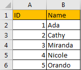
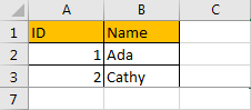
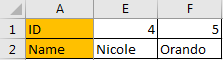
Suppose it lists a long list of ID and names. Header ID and Name are listed on the top. Now let’s freeze the first row.

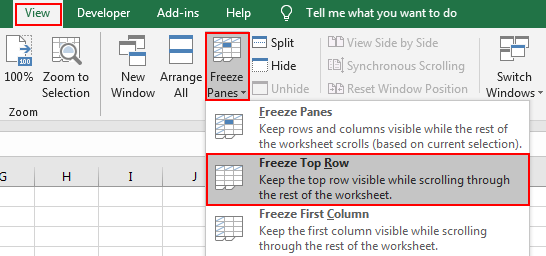
Step 1: Click View in the ribbon, then click Freeze Panes in Window group, then click the small triangle of Freeze Panes to load below three options, select the middle one ‘Freeze Top Row’.

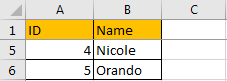
Step 2: After above operating. The first top row is fixed and always displayed on the top. Try to drag the scrollbar. You can see the header row is stayed on the top.

Method 2: How to Freeze Multiple Rows in Excel Spreadsheet

---

If you want to freeze the first three rows in excel, you can just select the first cell in the fourth row, then freeze the rows above the selected cell. See details below.

Step 1: Click A4 in the table.

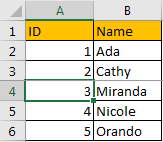
Step 2: Click View in the ribbon, then click Freeze Panes in Window group, then click the small triangle of Freeze Panes to load below three options, select the first one ‘Freeze Panes’.

Step 3: Try to drag the scrollbar. Verify that top three rows are fixed.

Method 3: How to Freeze the First Column in Excel Spreadsheet

---

See screenshot below:

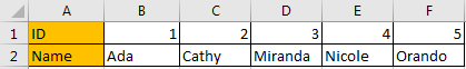
Now let’s freeze the first column. The way is similar with freeze the first row.

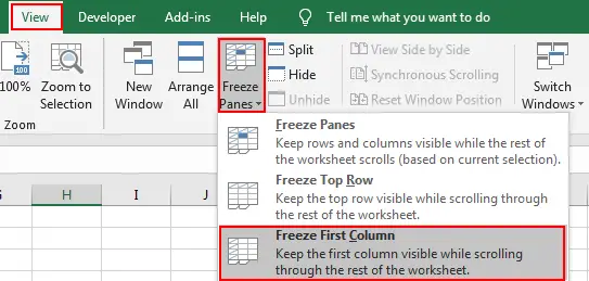
Step 1: Click View in the ribbon, then click Freeze Panes in Window group, then click the small triangle of Freeze Panes to load below three options, select the middle one ‘Freeze First Column’.

Step 2: Verify if it works well.

Obviously, it works.

Method 4: How to Freeze Row and Column in Excel Spreadsheet

---

If you want to just freeze the first row and column, just click on B2. Then click View->Freeze Panes->Freeze Panes in Window group.

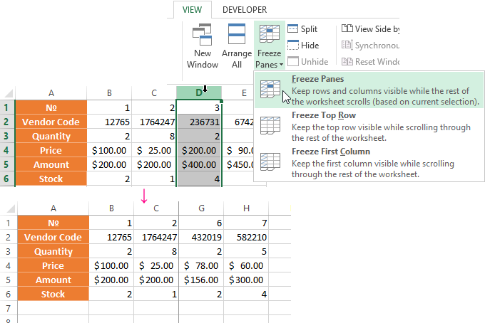
Method 5: How to Freeze Rows and Columns in Excel Spreadsheet

---

If you want to freeze multiple rows and columns, refer to the description of Freeze Panes ‘Keep rows and column visible while the rest of the worksheet scrolls (based on current selection)’ we can know that we can select a cell to make it as the first cell outside of your fixed area. For example, if we want to freeze the top three rows and first two columns (row 4 is not fixed and column C is not fixed), we can click on C4, then repeat above steps to freeze panes.