Lock one column in excel - Word и Excel - помощь в работе с программами

Freeze panes to lock rows and columns

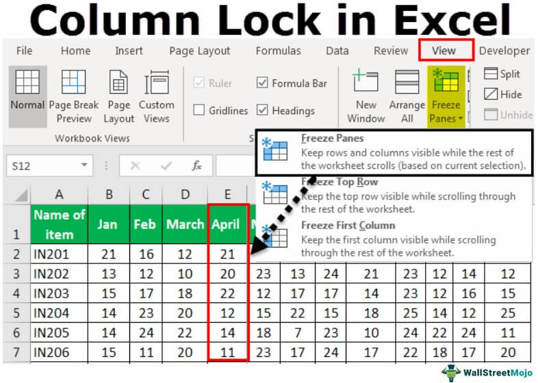
To keep an area of a worksheet visible while you scroll to another area of the worksheet, go to the View tab, where you can Freeze Panes to lock specific rows and columns in place, or you can Split panes to create separate windows of the same worksheet.

Freeze rows or columns

Freeze the first column

Select View > Freeze Panes > Freeze First Column.

The faint line that appears between Column A and B shows that the first column is frozen.

Freeze the first two columns

Select the third column.
Select View > Freeze Panes > Freeze Panes.

Freeze columns and rows

Select the cell below the rows and to the right of the columns you want to keep visible when you scroll.
Select View > Freeze Panes > Freeze Panes.

Unfreeze rows or columns

On the View tab > Window > Unfreeze Panes.

Note: If you don’t see the View tab, it’s likely that you are using Excel Starter. Not all features are supported in Excel Starter.

Need more help?

You can always ask an expert in the Excel Tech Community or get support in the Answers community.

The column lock feature in Excel is used to avoid any mishaps or undesired changes in data made by mistake by any user. We can apply this feature to a single column or multiple columns at once or separately. After selecting the desired column, change the formatting of the cells from locked to unlocked and password protect the workbook, which will not allow any user to change the locked columns.

For example, suppose we need to allow editing for necessary cells in an Excel spreadsheet but need not want others to edit cells containing essential data such as company information, formulas, drop-down lists, etc. Using this Excel feature, we can protect (lock) specific cells, columns, or rows on our Excel spreadsheet hassle-free and without any extra effort.

Locking a column can be done in two ways. We can do this by using the freeze panes in ExcelFreezing panes in excel helps freeze one or more rows and/or columns so that they remain fixed while scrolling through the database.read more and by protecting the worksheet by using the review functions of Excel. In Excel, we may want to lock a column so that the column does not disappear in case the user scrolls the sheet. That mainly happens when we have a large count of headers in a single sheet, and the user needs to scroll the sheet to see the other information.

When the user scrolls the data, some columns may lapse and not be visible to the user. So, we can lock the columns from getting scrolled out for the visible area.

Excel Column Lock
- How to Lock Column in Excel?
  - #1 – Locking the First Column of Excel
  - #2 – Lock any other Column of Excel
  - #3 – Using the Protect Sheet Feature to Lock a Column
- Explanation of Column Lock in Excel
- Things to Remember
- Recommended Articles

You are free to use this image on your website, templates, etc, Please provide us with an attribution linkArticle Link to be Hyperlinked
For eg:
Source: Column Lock in Excel (wallstreetmojo.com)

How to Lock Column in Excel?

#1 – Locking the First Column of Excel

Let us start.

We must go to the View tab from the ribbon and choose the option of Freeze Panes.
From the Freeze Panes options, choose the option of Freeze First Column.

As a result, this will freeze the first column of the spreadsheet.

#2 – Lock any other Column of Excel

If the column is to be locked, we need to follow the below steps.

Step #1 – We must select the column that needs to be locked. If we want to lock column “D,” we must choose the “E” column.

Step #2 – From the “View” tab, we must choose the “Freeze Pane” option and select the first option to lock the cell.

The output is shown below:

#3 – Using the Protect Sheet Feature to Lock a Column

In this case, the user will not be able to edit the content of the locked column.

Step #1 – Select the complete sheet and change the “Protection” to unlocked cells.

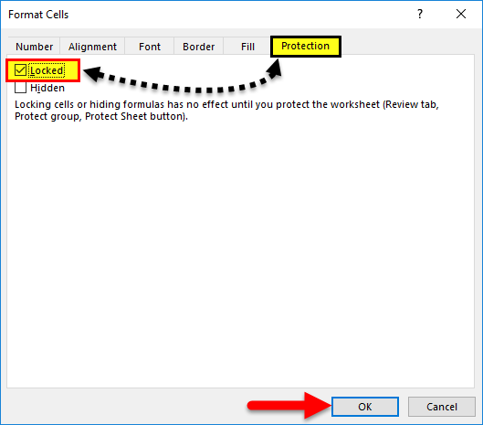
Step #2 – Now, we must select the column that we want to lock and change the property of that cell to “Locked.”

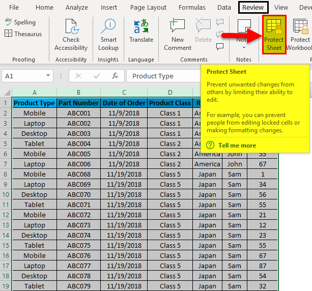
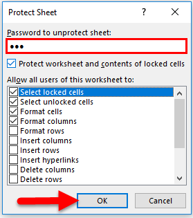
Step #3 – We must go to the “Review” tab and click on the “protect sheetWhen we don’t want any other user to make changes to our worksheet, we can use the Protect worksheet feature in Excel. It can be found in Excel’s Review tab. read more,” and then click on “OK.” Now, it will lock the column.

Explanation of Column Lock in Excel

Have you ever wondered what will happen if someone changes the value of a cell or a complete column? Yes, this may happen, especially in cases where the sheet is shared with multiple team users.

If this happens, this may drastically change the sheet’s data, as many other columns may depend upon the values of another column.

So, if we share our file with other users, we must ensure that the column is protected and no user can change the value of that column. We can do this by protecting the columns and hence locking their columns. If we lock a column, we can choose to have a password to unlock a column or prefer to continue without a password.

It is about locking the column, but sometimes we want a specific column that does not lapse in case the sheet is scrolled and always visible on the sheet.

In this case, we need to use the “Freeze Panes” option in Excel. Using this option, we can fix the position of a column. As a result, this position does not change even if the sheet is scrolled. Using the freeze panes, we can lock the first column, any other column, or even lock the rows and columns of ExcelA cell is the intersection of rows and columns. Rows and columns make the software that is called excel. The area of excel worksheet is divided into rows and columns and at any point in time, if we want to refer a particular location of this area, we need to refer a cell.read more.

Things to Remember

If we lock a column using the “Freeze Panes” option, only the column is locked from scrolling, and we can always change the column’s content anytime.
If we are using the “Protect Sheet” and the “Freeze Panes” options, then it is only possible to protect the column’s content and protect it from scrolling.
If we want a column that is not the first column to freeze, we need to select the next right column, and then we need to click on “Freeze Panes.” Hence, we should always choose the next column to freeze the previous column.
We can choose to have a password if we protect a column or continue without a password.

Lock Column in Excel

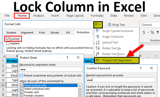
To lock a column in Excel, we first need to select the column we need to Lock. Then click right anywhere on the selected column and select the Format Cells option from the right-click menu list. Now from the Protection tab of Format Cells, check the box of LOCKED with a tick. There is another way to lock a column which can be done using the Protect Sheet option available under the Review menu tab. First, select the column which wants to lock, then use Protect Sheet with a password to lock it.

How to Lock Column in Excel?

To Lock a column in excel is very simple and easy. Let’s understand how to Lock Columns in Excel with some examples.

You can download this Lock Column Excel Template here – Lock Column Excel Template

Example #1

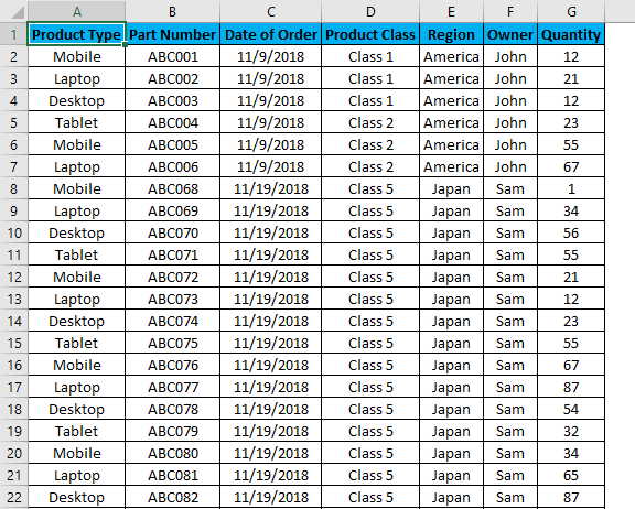
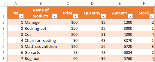
We got sample sales data from some products. Where we have observed that the Product Type column many times got changed by multiple logins. So, to avoid this, we are going to lock that Product Type column so that no one will change it. And data available after it will be accessible for changes. Below is the screenshot of available data for locking the required column.

For this purpose, first, select a cell or column which we need to protect, and then go to the Review tab and click on Protect Sheet.

Once we click on Protect Sheet, we will get a dialog box of Protect Sheet where we need to set a Password of any digit. Here we have set the password as 123.

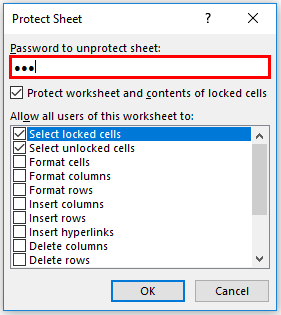
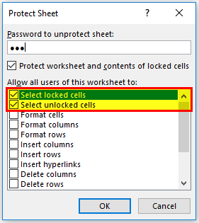
And check (tick) the options available in a box as per requirement. For example, I have checked selective locked cells and selected unlocked cells (which sometimes comes as default).

Once we are done with selecting the options for protecting the sheet or column, click on OK as highlighted below.

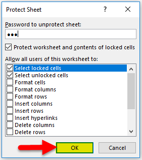
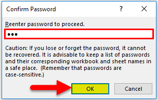
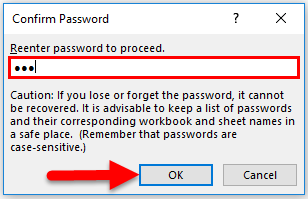
Once clicked on OK, the system will ask you to re-enter the password again. Once fed the password, click OK.

Now selected Column is locked, and no one can change anything in it without disabling the column’s protection.

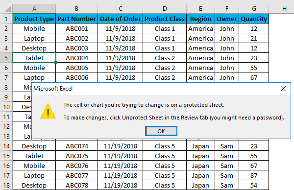
Let’s check whether the column is actually protected now. We had chosen Column A named as Product Type as required. For checking it, try to go in edit mode for any cell of that column (By Pressing F2 or double click); if it is protected, we will see a warning message as below.

Hence, our column data is now protected successfully.

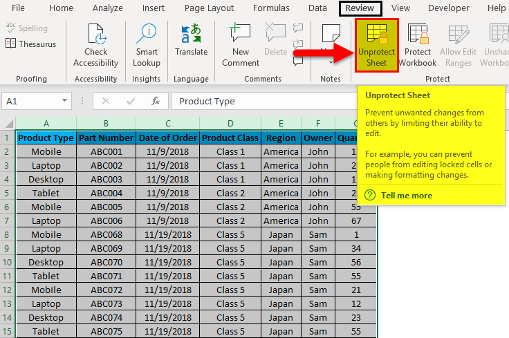
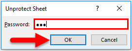
For unprotecting it again, go to the Review tab and click on the Unprotect Sheet, as shown below.

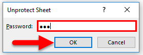
Once we click on the Unprotect Sheet, it will again ask for the same password to unprotect it. For that, re-enter the same password and click on Ok.

Now the column is unprotected, and we can make changes to it. We can also check the column whether it is accessible or not.

Example #2

Apart from the method which we have seen in the above example, we can lock any column in excel by this too. In this method, we will lock the desired column by using the Format Cell in Excel. If you are using this function for the first time, you will see your entire sheet selected as Locked to check-in Format cell. For that, select the entire sheet and go to the Home menu and Click the Orientation icon as shown below.

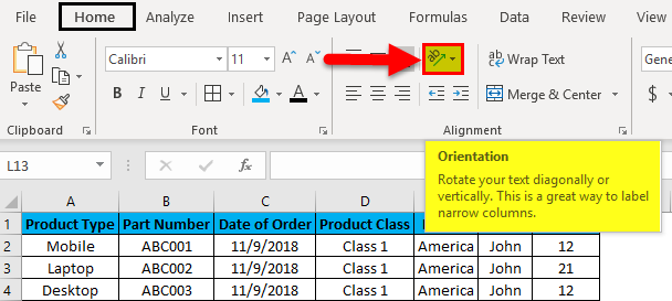
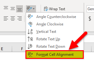
After that, a drop-down will appear. From there, click on Format Cell Alignment, as shown below.

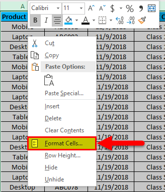
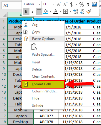
Format Cell Alignment can be accessed from different methods as well. This one is a shortcut approach for doing it. For this, select the entire sheet and Right Click anywhere. We will have the Format Cells option from right-click menu, as shown in the below screenshot. Click on it.

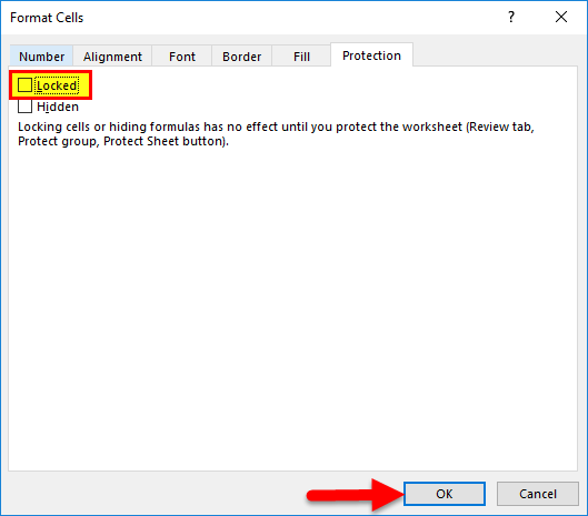
Once we click on it, we will get a dialog box of Format Cell. From there, go to the Protection tab.

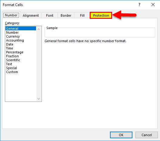
If you find the Locked box is already checked in (which is the default set), then uncheck it click on OK as shown below.

By doing this, we are clearing the default setting and customizing the sheet/column to protect it. Now select the column which we want to lock in excel. Here we are locking column A named as Product Type. Right-click on the same column, and select the Format Cell option.

After that, we will see the Format Cell box; go to the Protection Tab and Check-in Locked box. And again, click on OK, as shown below.

Follow the same procedure as explained in example-1. Refer to the below screenshot.

Re-enter the password and click on Ok.

For checking, we already chosen Column A named as Product Type as most of the time, the data available in Product Type gets disturbed. If it is protected, we will see a warning message as below.

So, we will have our column data protected and locked for making any changes.

For unprotecting it again, follow the same procedure as explained in example-1, as shown below.

Once we click on the Unprotect Sheet, it will again ask for the same password to unprotect it. For that, re-enter the same password and click on OK.

Now the column is unprotected, and we can make changes to it. We can also check the column whether it is accessible or not.

Pros of Excel Column Lock

It helps in data protection by not allowing any unauthorized person to make any changes.
Sometimes data is so confidential that, even if a file is shared with someone outside the company, then also a person will not be able to do anything, as the sheet/column is locked.

Cons of Excel Column Lock

Sometimes sheet gets so locked that, even in an emergency, we would not be able to change anything.
If we forget the password, then also there is no way to make changes in data. There will be only one way to create a new file with the same data to proceed further.

Things to Remember

Always note the password if you cannot remember it in the long future use.
Always have a backup of the file which is locked, without any password, so that it will be used further.
There are no criteria for creating a password.

How do I freeze specific columns in Excel?

To freeze columns:

Select the column to the right of the column(s) you want to freeze.
Click the View tab on the Ribbon.
Select the Freeze Panes command, then choose Freeze Panes from the drop-down menu.
The column will be frozen in place, as indicated by the gray line.

How do I freeze the first two columns in Excel?

Freeze columns and rows

Select the cell below the rows and to the right of the columns you want to keep visible when you scroll.
Select View > Freeze Panes > Freeze Panes.

How do I lock a variable in Excel?

Select the formula cell, click on one of the cell reference in the Formula Bar, and press the F4 key. Then the selected cell reference is locked.

How do you create a constant in Excel?

Name an array constant

Click Formulas > Define Name.
In the Name box, enter a name for your constant.
In the Refers to box, enter your constant.
Click OK.
In your worksheet, select the cells that will contain your constant.
In the formula bar, enter an equal sign and the name of the constant, such as =Quarter1.

Why is Excel not freezing the panes that I select?

Unfreeze Worksheet Pane:
For this, you should click to the View tab and then from the Window group, you should select the Freeze Panes arrow sign. Now from the drop-down menu, you should select the “Unfreeze Panes”. This method helps in fixing the issue.

How do you keep a column in Excel?

1. In an open spreadsheet, select “View” from the top menu bar and then hit “Freeze First Column.” This will freeze column A. 2. If you want to freeze multiple columns, click in the first cell to the right of the last column that you want to freeze.

How do I freeze two columns in Excel 2021?

If you want to freeze multiple columns in Excel, you do that in the same way as you would freeze multiple rows.

Select the column to the right of the column you want to freeze.
Select the View tab and Freeze Panes.
Select Freeze Panes.

How do I keep a row constant in Excel?

To freeze the top row or first column:

From the View tab, Windows Group, click the Freeze Panes drop down arrow.
Select either Freeze Top Row or Freeze First Column.
Excel inserts a thin line to show you where the frozen pane begins.

How do I lock a column and row in Excel?

Here are the steps to Lock Cells with Formulas:

With the cells with formulas selected, press Control + 1 (hold the Control key and then press 1).
In the format cells dialog box, select the Protection tab.
Check the ‘Locked’ option.
Click ok.

How do I freeze a row and a column in Excel at the same time?

Freeze rows or columns

To lock one row only, choose the View tab, and then click Freeze Top Row.
To lock one column only, choose the View tab, and then click Freeze First Column.
To lock more than one row or column, or to lock both rows and columns at the same time, choose the View tab, and then click Freeze Panes.

What is an Excel constant?

A constant is a set value that doesn’t change and that’s directly inserted into a cell. It’s not a formula and it’s not calculated by a formula.

What is an Xlookup in Excel?

Use the XLOOKUP function to find things in a table or range by row.With XLOOKUP, you can look in one column for a search term, and return a result from the same row in another column, regardless of which side the return column is on.

What is a constant in Excel example?

A constant is a value that doesn’t change (or rarely changes). Because a constant doesn’t change, you could just enter the value right into the formula. For instance, if you want to determine 10% commission on sales, you could use the formula =Sales*. 10.

What should you do if there are columns you need but do not want to display quizlet?

What should you do if there are columns you need, but do not want to display? Hide the columns you do not want to display, then unhide them when finished.

What is column freezing?

Freeze panes is a feature in spreadsheet applications, such as Microsoft Excel, LibreOffice Calc, and Google Sheets. It “freezes” a row or column, so that it is always displayed, even as you navigate the spreadsheet.

How do I freeze the top row and first column in Excel 2021?

Click on the View tab of the ribbon and select the option for Freeze Panes which will open a drop down menu. From here you will be able to select both columns and rows. 3. A thick black line will appear on the row above and on the column to the left of the active cell and all cells above this line will be frozen.

How do I freeze the top 2 rows in Excel 2021?

Click on the “View” tab at the top and select the “Freeze Panes” command. This will create a dropdown menu. From the options listed, select “Freeze Top Row.” This will freeze the first row, no matter what row you happen to have currently selected.

Источник

The Microsoft Excel program is designed not only to enter data into the table conveniently and edit it as you need it, but also to view large blocks of information. Most people using PCs work with it constantly.

The columns and rows names can be significantly removed from the cells with which the user is working at this time. Scrolling the page to see the name of the document is not comfortable for any user. Therefore, the Tabular Processor has possibilities to fix certain areas.

Locking a row in Excel while scrolling

Usually an Excel table has one cap. Meanwhile, this document can have up to thousands of rows. Working with multipage table blocks is inconvenient when column names are not visible. Scrolling the page to its beginning to return to the correct cell is absolutely irrational. To make the cap visible when scrolling, fix the top row of the Excel table, following these actions:

Create the needed table and fill it with the data.

data.

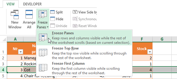
Make any of the cells active. Go to the “VIEW” tab using the tool “Freeze Panes”.

VIEW.

In the menu select the “Freeze Top Row” functions.

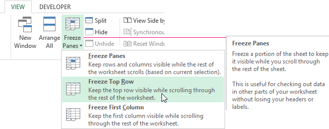
You will get a delimiting line under the top line. Now when you scroll vertically the table cap will be always visible.

Locking several rows in Excel while scrolling

Let us suppose, a user needs to fix not only the cap. For instance, another row or even a couple of rows must be fixed when scrolling the document. Doing it is possible and easy, when you follow these steps:

Select any cell under the line, which we will fix. This action will help Excel to “understand”, which area should be fixed;
Now select the “Freeze Panes” tool.

tool.

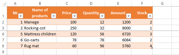
When you perform horizontal and vertical scrolling, the cap and the top row of the table remain fixed. Thus, you can fix two, three, four and more rows.

Note: This method works for 2007 and 2010 Excel versions. In earlier versions the “Lock areas” tool is located in the “Window” menu on the main page. There you must always (!) activate the cell under the freeze row.

Freezing columns in Excel

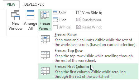
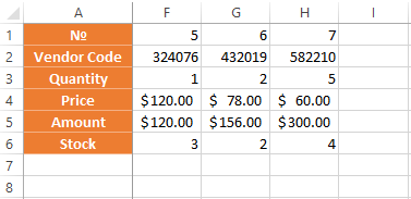
For instance, the information in the table has a horizontal direction. It is not concentrated in columns, but located in rows. For his comfort, the user must freeze the first column, containing the lines’ names in horizontal scrolling.

Select any cell of the chosen table so that Excel understands with what data it will work. Pin the first column in the menu you will see..

Now, when the document is scrolled to the right horizontally, the needed column will be fixed.

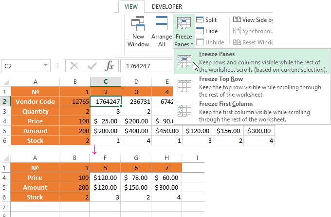
To freeze several columns, select the cell at the page bottom (to the right from the fixed column). Pick the “Freeze Panes” button.

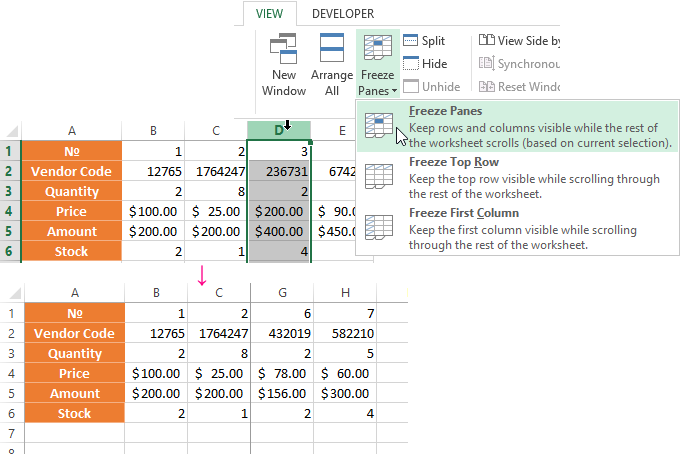
How to freeze the row and column in Excel

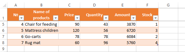
You have a task – to freeze the selected area, which contains two columns and two rows.

Make a cell at the intersection of the fixed rows and columns active. However, the cell must be not placed in the fixed area. It should have the position right under the required lines (to the right of the required columns). Pick the first option in Excel Locking Areas. The photo shows that when scrolling, the selected areas remain at the same place.

Removing a fixed area in Excel

After fixing a row or a column of the table the button deleting all pivot tables becomes available.

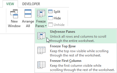
After clicking – «Unfreeze Panes», all the locked areas of the worksheet become unlocked.

Источник

Freeze rows or columns

Unfreeze rows or columns

Need more help?

See Also

Need more help?

Want more options?

Table of contents

How to Lock Column in Excel?

#1 – Locking the First Column of Excel

#2 – Lock any other Column of Excel

#3 – Using the Protect Sheet Feature to Lock a Column

Explanation of Column Lock in Excel

Things to Remember

Recommended Articles

Lock Column in Excel

How to Lock Column in Excel?

Example #1

Example #2

Pros of Excel Column Lock

Cons of Excel Column Lock

Things to Remember

Recommended Articles

How do I freeze specific columns in Excel?

How do I freeze the first two columns in Excel?

How do I lock a variable in Excel?

How do you create a constant in Excel?

Why is Excel not freezing the panes that I select?

How do you keep a column in Excel?

How do I freeze two columns in Excel 2021?

How do I keep a row constant in Excel?

How do I lock a column and row in Excel?

How do I freeze a row and a column in Excel at the same time?

What is an Excel constant?

What is an Xlookup in Excel?

What is a constant in Excel example?

What should you do if there are columns you need but do not want to display quizlet?

What is column freezing?

How do I freeze the top row and first column in Excel 2021?

How do I freeze the top 2 rows in Excel 2021?

Locking a row in Excel while scrolling

Locking several rows in Excel while scrolling

Freezing columns in Excel

How to freeze the row and column in Excel

Removing a fixed area in Excel