
Suppose that your boss wants you to protect an entire workbook, but also wants to be able to change a few cells after you enable protection on the workbook. Before you enabled password protection, you had unlocked some cells in the workbook. Now that your boss is done with the workbook, you can lock these cells.
Follow these steps to lock cells in a worksheet:
-
Select the cells you want to lock.
-
On the Home tab, in the Alignment group, click the small arrow to open the Format Cells popup window.
-
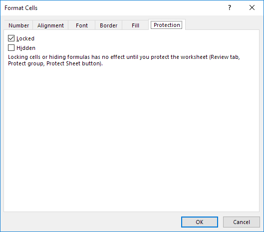
On the Protection tab, select the Locked check box, and then click OK to close the popup.
Note: If you try these steps on a workbook or worksheet you haven’t protected, you’ll see the cells are already locked. This means that the cells are ready to be locked when you protect the workbook or worksheet.
-
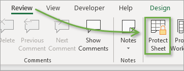
On the Review tab in the ribbon, in the Changes group, select either Protect Sheet or Protect Workbook, and then reapply protection. See Protect a worksheet or Protect a workbook.
Tip: It’s a best practice to unlock any cells that you may want to change before you protect a worksheet or a workbook, but you can also unlock them after you apply protection. To remove protection, simply remove the password.
In addition to protecting workbooks and worksheets, you can also protect formulas.
Excel for the web can’t lock cells or specific areas of a worksheet.
If you want to lock cells or protect specific areas, click Open in Excel and lock cells to protect them or lock or unlock specific areas of a protected worksheet.
Содержание
- How to lock cells in Excel
- How to lock all the cells in an Excel worksheet
- How to Lock Specific Cells in an Excel Worksheet
- More Microsoft Excel tips and tricks
- Be In the Know
- Lock cells to protect them
- Need more help?
- Lock Cells
- Lock All Cells
- Lock Specific Cells
- Lock Formula Cells
- How to lock and unlock cells in Excel
- How to lock cells in Excel
- 1. Unlock all cells on the sheet
- 2. Select cells, ranges, columns or rows you want to protect
- 3. Lock selected cells
- 4. Protect the sheet
- How to unlock cells in Excel (unprotect a sheet)
- How to unlock certain cells on a protected Excel sheet
- Allow certain users to edit selected cells without password
- How to lock cells in Excel other than input cells
- How to find and highlight locked / unlocked cells on a sheet
How to lock cells in Excel
This is how to protect cells in Excel
You’ve worked hard on your spreadsheet and now you want to make sure anyone you share it with doesn’t inadvertently change cells, so you need to know how to lock cells in Excel.
Thankfully, Microsoft Excel 2016 and earlier versions lets you lock cells or protect cells to keep them from being modified in Windows 10. You can lock all the cells in a worksheet or specific cells, allowing some parts of the spreadsheet to be changed. Here’s how to lock cells in Excel.
Editor’s Note: This tutorial was written for Excel 2016, but still applies to modern versions of Excel.
How to lock all the cells in an Excel worksheet

By default, when you protect cells in a sheet or workbook, all of the cells will be locked. This means they can’t be reformatted or deleted, and the content in them can’t be edited. By default, the locked cells can be selected, but you can change that in the protection options.
1. Navigate to the Review tab.
2. Click Protect Sheet. In the Protect Sheet window, enter a password that’s required to unprotect the sheet (optional) and any of the actions you want to allow users.
3. Click OK to protect the sheet.
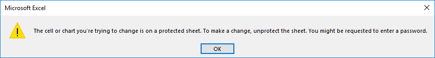
When you or anyone else tries to edit any of the locked cells, this message will come up:
The cells can only be unlocked when the sheet is unprotected (by going to the Review tab again, choosing «Unprotect Sheet,» and entering the password, if required).
How to Lock Specific Cells in an Excel Worksheet
There might be times when you want to lock certain cells from being changed but still allow users to adjust other cells in a worksheet. In our example, in an inventory list you might allow unit prices and stock quantities to be updated, but not the item IDs, names, or descriptions. As mentioned above, all cells are locked by default when you protect the sheet. However, you can specify whether a certain cell should be locked or unlocked in the cell’s format properties.
1. Select all the cells you don’t want to be locked. These will be the specific cells that can be edited even after the sheet is protected.
2. Right-click on your selection, select Format Cells, and click on the Protection tab. (Alternatively, under the Home tab, click on the expansion icon next to Alignment, and in the Format Cells window go to the Protection tab.)
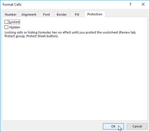
3. Uncheck «Locked» (which is checked by default) and click OK.
4. Go to Review > Protect Sheet and hit OK to protect the sheet. Any cells you didn’t unlock under the Format Cells option (step 3 above) will be locked, while the unlocked cells will be editable:
Note that locking (or unlocking) specific cells won’t take effect until you do step 4, protecting the sheet.
Protip: If you want to quickly lock or unlock cells that aren’t next to each other, you can use a keyboard shortcut. After selecting a certain cell or group of cells, use the Format Cells dialog as above to lock or unlock it. Then select your next cell(s) and hit F4 to repeat your last action.
More Microsoft Excel tips and tricks
There are a number of neat tips that’ll help you out when you’re managing your Excel spreadsheets. For example, we have a guide on how to use VLOOKUP in Excel, which you can use to to quickly find data associated with a value the user enters. And if you need to, you can also freeze rows and columns by selecting «Freeze Panes» in the View tab. If you need to organize your data, check out how to create sortable columns in Excel.
But, not everyone is a fan of Excel, so if you need to convert Excel Spreadsheets to Google Sheets, we have a guide for that, as well as a guide on how to open Google Sheets in Excel.
If you’re a business users, we also have 10 Excel business tips that you can use to help you keep your job, which include guides on how to remove duplicate data, recover lost Excel files, use pivot tables to summarize data and more.
Be In the Know
Get instant access to breaking news, the hottest reviews, great deals and helpful tips.
By submitting your information you agree to the Terms & Conditions (opens in new tab) and Privacy Policy (opens in new tab) and are aged 16 or over.
Источник
Lock cells to protect them
Suppose that your boss wants you to protect an entire workbook, but also wants to be able to change a few cells after you enable protection on the workbook. Before you enabled password protection, you had unlocked some cells in the workbook. Now that your boss is done with the workbook, you can lock these cells.
Follow these steps to lock cells in a worksheet:
Select the cells you want to lock.
On the Home tab, in the Alignment group, click the small arrow to open the Format Cells popup window.
On the Protection tab, select the Locked check box, and then click OK to close the popup.
Note: If you try these steps on a workbook or worksheet you haven’t protected, you’ll see the cells are already locked. This means that the cells are ready to be locked when you protect the workbook or worksheet.
On the Review tab in the ribbon, in the Changes group, select either Protect Sheet or Protect Workbook, and then reapply protection. See Protect a worksheet or Protect a workbook.
Tip: It’s a best practice to unlock any cells that you may want to change before you protect a worksheet or a workbook, but you can also unlock them after you apply protection. To remove protection, simply remove the password.
In addition to protecting workbooks and worksheets, you can also protect formulas.
Excel for the web can’t lock cells or specific areas of a worksheet.
If you want to lock cells or protect specific areas, click Open in Excel and lock cells to protect them or lock or unlock specific areas of a protected worksheet.
Need more help?
You can always ask an expert in the Excel Tech Community or get support in the Answers community.
Источник
Lock Cells
You can lock cells in Excel if you want to protect cells from being edited.
Lock All Cells
By default, all cells are locked. However, locking cells has no effect until you protect the worksheet.
1. Select all cells.
2. Right click, and then click Format Cells (or press CTRL + 1).
3. On the Protection tab, you can verify that all cells are locked by default.
4. Click OK or Cancel.
All cells are locked now. To unprotect a worksheet, right click on the worksheet tab and click Unprotect Sheet. The password for the downloadable Excel file is «easy».
Lock Specific Cells
To lock specific cells in Excel, first unlock all cells. Next, lock specific cells. Finally, protect the sheet.
1. Select all cells.
2. Right click, and then click Format Cells (or press CTRL + 1).
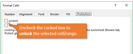
3. On the Protection tab, uncheck the Locked check box and click OK.
4. For example, select cell A1 and cell A2.
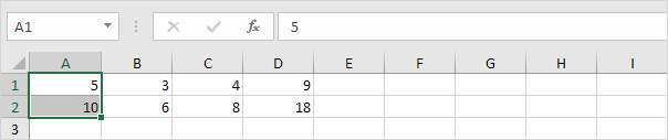
5. Right click, and then click Format Cells (or press CTRL + 1).
6. On the Protection tab, check the Locked check box and click OK.

Again, locking cells has no effect until you protect the worksheet.
Cell A1 and cell A2 are locked now. To edit these cells, you have to unprotect the sheet. The password for the downloadable Excel file is «easy». You can still edit all other cells.
Lock Formula Cells
To lock all cells that contain formulas, first unlock all cells. Next, lock all formula cells. Finally, protect the sheet.
1. Select all cells.
2. Right click, and then click Format Cells (or press CTRL + 1).
3. On the Protection tab, uncheck the Locked check box and click OK.
4. On the Home tab, in the Editing group, click Find & Select.
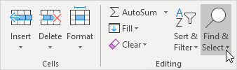
5. Click Go To Special.

6. Select Formulas and click OK.
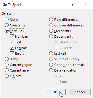
Excel selects all formula cells.
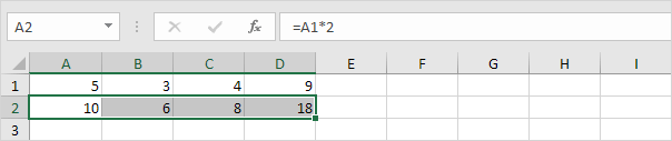
7. Press CTRL + 1.
8. On the Protection tab, check the Locked check box and click OK.

Note: if you also check the Hidden check box, users cannot see the formula in the formula bar when they select cell A2, B2, C2 or D2.
Again, locking cells has no effect until you protect the worksheet.
All formula cells are locked now. To edit these cells, you have to unprotect the sheet. The password for the downloadable Excel file is «easy». You can still edit all other cells.
Источник
How to lock and unlock cells in Excel
 by Svetlana Cheusheva, updated on February 7, 2023
The tutorial explains how to lock a cell or certain cells in Excel to protect them from deleting, overwriting or editing. It also shows how to unlock individual cells on a protected sheet by a password, or allow specific users to edit those cells without password. And finally, you will learn how to detect and highlight locked and unlocked cells in Excel.
In last week’s tutorial, you learned how to protect Excel sheets to prevent accidental or deliberate changes in the sheet contents. However, in some cases you may not want to go that far and lock the entire sheet. Instead, you can lock only specific cells, columns or rows, and leave all other cells unlocked.
For example, you can allow your users to input and edit the source data, but protect cells with formulas that calculate that data. In other words, you may want to only lock a cell or range that shouldn’t be changed.
How to lock cells in Excel
Locking all cells on an Excel sheet is easy — you just need to protect the sheet. Because the Locked attributed is selected for all cells by default, protecting the sheet automatically locks cells.
If you don’t want to lock all cells on the sheet, but rather want to protect certain cells from overwriting, deleting or editing, you will need to unlock all cells first, then lock those specific cells, and then protect the sheet.
The detailed steps to lock cells in Excel 365 — 2010 follow below.
1. Unlock all cells on the sheet
By default, the Locked option is enabled for all cells on the sheet. That is why, in order to lock certain cells in Excel, you need to unlock all cells first.
- Press Ctrl + A or click the Select All button
 to select the entire sheet.
 - Press Ctrl + 1 to open the Format Cells dialog (or right-click any of the selected cells and choose Format Cells from the context menu).
- In the Format Cells dialog, switch to the Protection tab, uncheck the Locked option, and click OK.
 to select the entire sheet.
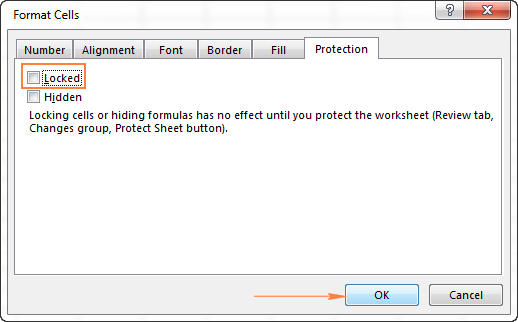
2. Select cells, ranges, columns or rows you want to protect
To lock cells or ranges, select them in a usual way by using the mouse or arrow keys in combination with Shift. To select non-adjacent cells, select the first cell or a range of cells, press and hold the Ctrl key, and select other cells or ranges.
To protect columns in Excel, do one of the following:
- To protect one column, click on the column’s letter to select it. Or, select any cell within the column you want to lock, and press Ctrl + Space .
- To select adjacent columns, right click on the first column heading and drag the selection across the column letters rightwards or leftwards. Or, select the first column, hold down the Shift key, and select the last column.
- To select non-adjacent columns, click on the first column’s letter, hold down the Ctrl key, and click the headings of other columns you want to protect.
To protect rows in Excel, select them in a similar manner.
To lock all cells with formulas, go to the Home tab > Editing group > Find & Select > Go To Special. In the Go To Special dialog box, check the Formulas radio button, and click OK. For the detailed guidance with screenshots, please see How to lock and hide formulas in Excel.
3. Lock selected cells
With the required cells selected, press Ctrl + 1 to open the Format Cells dialog (or right-click the selected cells and click Format Cells), switch to the Protection tab, and check the Locked checkbox. 
4. Protect the sheet
Locking cells in Excel has no effect until you protect the worksheet. This can be confusing, but Microsoft designed it this way, and we have to play by their rules 🙂
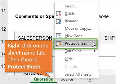
On the Review tab, in the Changes group, click the Protect Sheet button. Or, right click the sheet tab and select Protect Sheet… in the context menu. 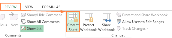
You will be prompted to enter the password (optional) and select the actions you want to allow users to perform. Do this, and click OK. You can find the detailed instructions with screenshots in this tutorial: How to protect a sheet in Excel.
Done! The selected cells are locked and protected from any changes, while all other cells in the worksheet are editable.
If you are working in Excel web app, then see how to lock cells for editing in Excel Online.
How to unlock cells in Excel (unprotect a sheet)
To unlock all cells on a sheet, it is sufficient to remove the worksheet protection. To do this, right-click the sheet tab, and select Unprotect Sheet… from the context menu. Alternatively, click the Unprotect Sheet button on the Review tab, in the Changes group: 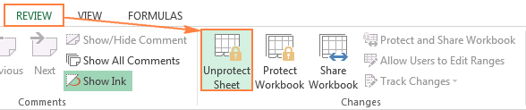
For more information, please see How to unprotect an Excel sheet.
As soon as the worksheet is unprotected, you can edit any cells, and then protect the sheet again.
If you want to allow users to edit specific cells or ranges on a password-protected sheet, check out the following section.
How to unlock certain cells on a protected Excel sheet
In the first section of this tutorial, we discussed how to lock cells in Excel so that no one even yourself can edit those cells without unprotecting the sheet.
However, sometimes you may want to be able to edit specific cells on your own sheet, or let other trusted users to edit those cells. In other words, you can allow certain cells on a protected sheet to be unlocked with password. Here’s how:
- Select the cells or ranges you want to unlock by a password when the sheet is protected.
- Go to the Review tab >Changes group, and click Allow Users to Edit Ranges.
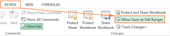
Note. This feature is available only in an unprotected sheet. If the Allow Users to Edit Ranges button is greyed out, click the Unprotect Sheet button on the Review tab.
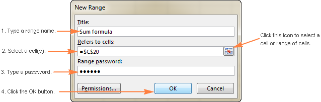
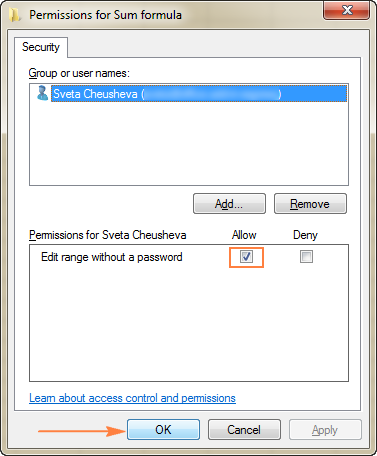
Tip. In addition to, or instead of, unlocking the specified range by a password, you can give certain users the permissions to edit the range without password. To do this, click the Permissions… button in the lower left corner of the New Range dialog and follow these guidelines (steps 3 — 5).
Tip. It is recommended to protect a sheet with a different password than you used to unlock the range(s). 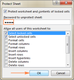
Now, your worksheet is password protected, but specific cells can be unlocked by the password you supplied for that range. And any user who knows that range password can edit or delete the cells contents.
Allow certain users to edit selected cells without password
Unlocking cells with password is great, but if you need to frequently edit those cells, typing a password every time can be a waste of your time and patience. In this case, you can set up permissions for specific users to edit some ranges or individual cells without password.
Note. This features works on Windows XP or higher, and your computer must be on a domain.
Assuming that you have already added one or more ranges unlockable by a password, proceed with the following steps.
- Go to the Review tab >Changes group, and click Allow Users to Edit Ranges.
Note. If the Allow Users to Edit Ranges is grayed out, click the Unprotect Sheet button to remove the worksheet protection.
Tip. The Permissions… button is also available when you are creating a new range unlocked by a password.
To see the required name format, click the examples link. Or, simply type the user name as it is stored on your domain, and click the Check Names button to verify the name.
For example, to allow myself to edit the range, I’ve typed my short name: 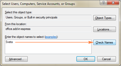
Excel has verified my name and applied the required format: 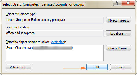
Note. If a given cell belongs to more than one range unlocked by a password, all users who are authorized to edit any of those ranges can edit the cell.
How to lock cells in Excel other than input cells
When you’ve put a lot of effort in creating a sophisticated form or calculation sheet in Excel, you will definitely want to protect your work and prevent users from tampering with your formulas or changing data that shouldn’t be changed. In this case, you can lock all cells on your Excel sheet except for input cells where your users are supposed to enter their data.
One of possible solutions is to use the Allow Users to Edit Ranges feature to unlock selected cells, as demonstrated above. Another solution could be modifying the built-in Input style so that it not only formats the input cells but also unlocks them.
For this example, we are going to use an advanced compound interest calculator that we created for one of the previous tutorials. This is how it looks like: 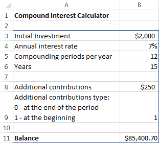
Users are expected to enter their data in cells B2:B9, and the formula in B11 calculates the balance based on the user’s input. So, our aim is to lock all cells on this Excel sheet, including the formula cell and fields’ descriptions, and leave only the input cells (B3:B9) unlocked. To do this, perform the following steps.
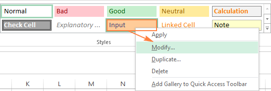
- On the Home tab, in the Styles group, find the Input style, right click it, and then click Modify….
- By default, Excel’s Input style includes information about the font, border and fill colors, but not the cell protection status. To add it, just select the Protection checkbox:
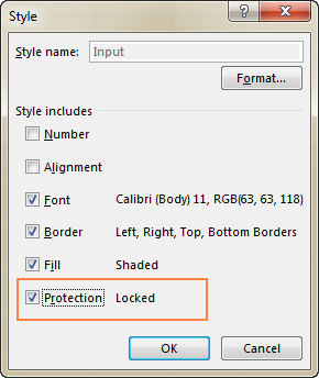
Tip. If you want only to unlock input cells without changing cell formatting, uncheck all boxes on the Style dialog window other than the Protection box.
If Excel’s Input style does not suit you for some reason, you can create your own style that unlocks selected cells, the key point is to select the Protection box and set it to No Protection, as demonstrated above.
How to find and highlight locked / unlocked cells on a sheet
If you have been locking and unlocking cells on a given spreadsheet multiple times, you may have forgotten which cells are locked and which are unlocked. To quickly find locked and unlocked cells, you can use the CELL function, which returns information about the formatting, location and other properties if a specified cell.
To determine the protection status of a cell, enter the word «protect» in the first argument of your CELL formula, and a cell address in the second argument. For example:
If A1 is locked, the above formula returns 1 (TRUE), and if it’s unlocked the formula returns 0 (FALSE) as demonstrated in the screenshot below (the formulas are in cells B1 and B2): 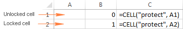
It cannot be easier, right? However, if you have more than one column of data, the above approach is not the best way to go. It would be far more convenient to see all locked or unlocked cells at a glance rather than sorting out numerous 1’s and 0’s.
The solution is to highlight locked and/or unlocked cells by creating a conditional formatting rule based on the following formulas:
- To highlight locked cells: =CELL(«protect», A1)=1
- To highlight unlocked cells: =CELL(«protect», A1)=0
Where A1 is the leftmost cell of the range covered by your conditional formatting rule.
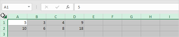
As an example, I’ve created a small table and locked cells B2:D2 that contain SUM formulas. The following screenshot demonstrates a rule that highlights those locked cells: 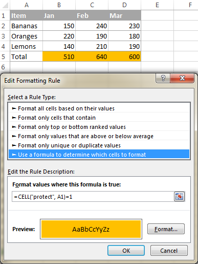
Note. The conditional formatting feature is disabled on a protected sheet. So, be sure to turn off the worksheet protection before creating a rule (Review tab > Changes group > Unprotect Sheet).
If you don’t have much experience with Excel conditional formatting, you may find the following step-by-step instructions helpful: Excel conditional formatting based on another cell value.
This is how you can lock one or more cells in your Excel sheets. If someone knows any other way to protect cells in Excel, your comments will be truly appreciated. I thank you for reading and hope to see you on our blog next week.
Источник
Lock All Cells | Lock Specific Cells | Lock Formula Cells
You can lock cells in Excel if you want to protect cells from being edited.
Lock All Cells
By default, all cells are locked. However, locking cells has no effect until you protect the worksheet.
1. Select all cells.
2. Right click, and then click Format Cells (or press CTRL + 1).
3. On the Protection tab, you can verify that all cells are locked by default.
4. Click OK or Cancel.
5. Protect the sheet.
All cells are locked now. To unprotect a worksheet, right click on the worksheet tab and click Unprotect Sheet. The password for the downloadable Excel file is «easy».
Lock Specific Cells
To lock specific cells in Excel, first unlock all cells. Next, lock specific cells. Finally, protect the sheet.
1. Select all cells.
2. Right click, and then click Format Cells (or press CTRL + 1).
3. On the Protection tab, uncheck the Locked check box and click OK.
4. For example, select cell A1 and cell A2.
5. Right click, and then click Format Cells (or press CTRL + 1).
6. On the Protection tab, check the Locked check box and click OK.
Again, locking cells has no effect until you protect the worksheet.
7. Protect the sheet.
Cell A1 and cell A2 are locked now. To edit these cells, you have to unprotect the sheet. The password for the downloadable Excel file is «easy». You can still edit all other cells.
Lock Formula Cells
To lock all cells that contain formulas, first unlock all cells. Next, lock all formula cells. Finally, protect the sheet.
1. Select all cells.
2. Right click, and then click Format Cells (or press CTRL + 1).
3. On the Protection tab, uncheck the Locked check box and click OK.
4. On the Home tab, in the Editing group, click Find & Select.
5. Click Go To Special.
6. Select Formulas and click OK.
Excel selects all formula cells.
7. Press CTRL + 1.
8. On the Protection tab, check the Locked check box and click OK.
Note: if you also check the Hidden check box, users cannot see the formula in the formula bar when they select cell A2, B2, C2 or D2.
Again, locking cells has no effect until you protect the worksheet.
9. Protect the sheet.
All formula cells are locked now. To edit these cells, you have to unprotect the sheet. The password for the downloadable Excel file is «easy». You can still edit all other cells.
![]()
Download Article
![]()
Download Article
Locking cells in an Excel spreadsheet can prevent any changes from being made to the data or formulas that reside in those particular cells. Cells that are locked and protected can be unlocked at any time by the user who initially locked the cells. Follow the steps below to learn how to lock and protect cells in Microsoft Excel versions 2010, 2007, and 2003.
To learn how to unlock the cells, read the article How to Open a Password Protected Excel File.
Things You Should Know
- In all versions of Excel, highlight and right click your cells. Then, select «Format Cells» > «Protection.» Check «Locked» and save.
- In Excel 2007 and 2010, go to «Review» > «Changes/Protect Sheet» > «Protect worksheet and contents of locked cells.» Type a password click through the prompts to save.
- In Excel 2003, go to «Tools» > «Protection» > «Protect Sheet.» Check «Protect worksheet and contents of locked cells.» Enter a password and follow the prompts to save.
-
1
Open the Excel spreadsheet that contains the cells you want locked.
-
2
Select the cell or cells you want locked.
Advertisement
-
3
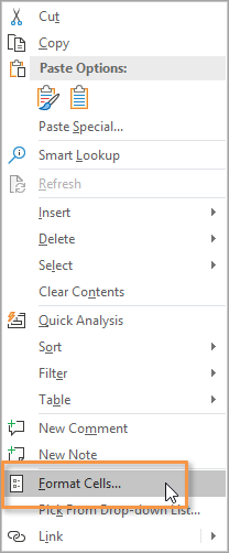
Right-click on the cells, and select «Format Cells.»
-
4
Click on the tab labeled «Protection.»
-
5
Place a checkmark in the box next to the option labeled «Locked.»
-
6
Click «OK.»
-
7
Click on the tab labeled «Review» at the top of your Excel spreadsheet.
-
8
Click on the button labeled «Protect Sheet» from within the «Changes» group.
-
9
Place a checkmark next to «Protect worksheet and contents of locked cells.»
-
10
Enter a password in the text box labeled «Password to unprotect sheet.»
-
11
Click on «OK.»
-
12
Retype your password into the text box labeled «Reenter password to proceed.»
-
13
Click «OK.» The cells you selected will now be locked and protected, and can only be unlocked by selecting the cells once again, and entering the password you selected.


Advertisement
-
1
Open the Excel document that contains the cell or cells you want to lock.
-
2
Select one or all of the cells you want locked.
-
3
Right-click on your cell selections, and select «Format Cells» from the drop-down menu.
-
4
Click on the «Protection» tab.
-
5
Place a checkmark next to the field labeled «Locked.»
-
6
Click the «OK» button.
-
7
Click on the «Tools» menu at the top of your Excel document.
-
8
Select «Protection» from the list of options.
-
9
Click on «Protect Sheet.»
-
10
Place a checkmark next to the option labeled «Protect worksheet and contents of locked cells.»
-
11
Type a password at the prompt for «Password to unprotect sheet,» then click «OK.»
-
12
Reenter your password at the prompt for «Reenter password to proceed.»
-
13
Select «OK.» All the cells you selected will now be locked and protected, and can only be unlocked going forward by selecting the locked cells, and entering the password you initially set up.


Advertisement
Add New Question
-
Question
How do I lock cells in Excel without the whole document becoming read only?

I suppose you want to lock certain cells instead of the whole sheets. To do that, choose the whole sheet, right click and then select «Format Cells», then «Protection», then uncheck the «Locked» option and click okay. Then select the cells you want to lock, right click and select «Format Cells», then Protection; this time, check the «Locked» option and click okay. Now go back to the main tab, select «Review», then click on «Protect Sheet», and do whatever you want to do with it. Now only the cells you «locked» are protected from editing instead of the whole sheet.
-
Question
How can I protract the single cell while using Excel?
You cannot protract a single cell in Excel. You can, however, make it appear longer than the rest of the cells around it by «merging» two or more cells together. Highlight the cells you desire and right click. A menu will pop up allowing you to merge them.
-
Question
How do I allow changes to some cells of a protected sheet?
Select the whole worksheet by clicking the Select All button. On the Home tab, in the Font group, click the Format Cell Font dialog box launcher. On the Protection tab, clear the Locked box and then click OK.
Ask a Question
200 characters left
Include your email address to get a message when this question is answered.
Submit
Advertisement
Video
-
If multiple users have access to your Excel document, lock all cells that contain important data or complex formulas to prevent the cells from being accidentally changed.
-
If the majority of cells in your Excel document contain valuable data or complex formulas, consider locking or protecting the entire document, then unlock the few cells that are allowed to be modified.
Thanks for submitting a tip for review!
Advertisement
About This Article
Article SummaryX
1. Select the cells.
2. Right-click the cells and select Format Cells.
3. Click Protection.
4. Check the ″Locked″ box and click OK.
5. Click Review.
6. Click Protect Sheet.
7. Check ″Protect worksheet and contents of locked cells.″
8. Enter a password and click OK.
Did this summary help you?
Thanks to all authors for creating a page that has been read 235,187 times.
Is this article up to date?
Bottom Line: Learn how to lock individual cells or ranges in Excel so that users cannot change the formulas or contents of protected cells. Plus a few bonus tips to save time with the setup.
Skill Level: Beginner
Video Tutorial
Download the Excel File
You can download the file that I use in the video tutorial by clicking below.
Protecting Your Work from Unwanted Changes
If you share your spreadsheets with other users, you’ve probably found that there are specific cells you don’t want them to modify. This is especially true for cells that contain formulas and special formatting.
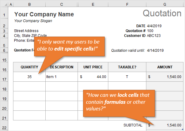
The great news is that you can lock or unlock any cell, or a whole range of cells, to keep your work protected. It’s easy to do, and it involves two basic steps:
- Locking/unlocking the cells.
- Protecting the worksheet.
Here’s how to prevent users from changing some cells.
Step 1: Lock and Unlock Specific Cells or Ranges
Right-click on the cell or range you want to change, and choose Format Cells from the menu that appears.
This will bring up the Format Cells window (keyboard shortcut for this window is Ctrl + 1.). Choose the tab that says Protection.
Next, make sure that the Locked option is checked.
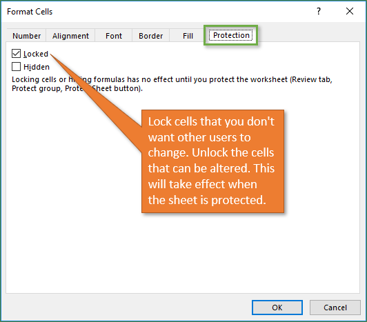
Locked is the default setting for all cells in a new worksheet/workbook.
Once we protect the worksheet (in the next step) those locked cells will not be able to be altered by users.
If you want users to be able to edit a particular cell or range, uncheck the Locked box so they are unlocked. Since cells are locked by default, most of the job will be going through the sheet and unlocking cells that can be edited by users.
I share some shortcuts to make this process faster in the Bonus section below.
Step 2: Protect the Worksheet
Now that you’ve locked/unlocked the cells that you want users to be able to edit, you want to protect the sheet. Once you protect the sheet, users cannot change the locked cells. However, they can still modify the unlocked cells.
To protect the sheet, simply right-click on the tab at the bottom of the sheet, and choose Protect Sheet… from the menu.
This will bring up the Protect Sheet window. If you want your sheet to be password protected, you have the option of entering a password here. Adding a password is optional. Click OK.
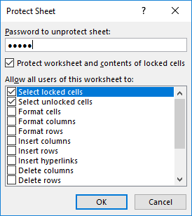
If you’ve chosen to enter a password, then you will be prompted to verify your entry after you’ve clicked OK.
With the sheet protected, users will be unable to change the cells that are locked. If they try to make changes, they will get an error/warning message that looks like this.
You can unprotect the sheet in the same way that you protected it, by right-clicking on the sheet tab. An alternative way to protect and unprotect sheets is by using the Protect Sheet button in the Review tab of the Ribbon.
The button text displays the opposite of the current state. It says Protect Sheet when the sheet is unprotected, and Unprotect Sheet when it is protected.
It’s important to note that all cells can be edited when the sheet is unprotected. After making changes you must protect the sheet again and Save the workbook before sending or sharing with other users.
3 Bonus Tips for Locking Cells and Protecting Sheets
As you can see, it is fairly simple to protect your formulas and formatting from being changed! But I’d like to leave you with three tips to help make it faster & easier for both you and your users.
1. Prevent Locked Cells From Being Selected
This tip will help make it faster and easier for your users to input data in the sheet.
Turning off the Select locked cells option prevents the locked cells from being selected with either the mouse or keyboard (arrow or tab keys). This means users will only be able to select the unlocked cells that they need to edit. They can quickly hit the Tab, Enter, or arrow keys to move to the next editable cell.
To make this change, you just uncheck the option that says “Select locked cells” on the Protect Sheet window.
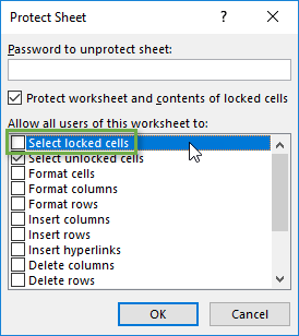
After pressing OK, you will only be able to select the unlocked cells.
2. Add a button for locking cells to the Quick Access Toolbar
This allows you to quickly see the locked setting for a cell or range.
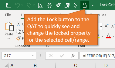
From the Home tab on the Ribbon, you can open the drop-down menu under the Format button and see the option to Lock Cell.
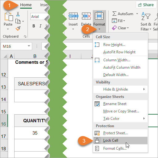
If you right-click on the Lock Cell option, another menu appears giving you the option to add the button to the Quick Access Toolbar.
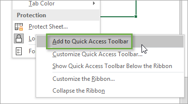
When you select this option, the button will be added to the Quick Access Toolbar at the top of the workbook. This button will remain each time you use Excel. You can easily lock and unlock specific cells on your sheet by clicking on this button.
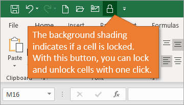
You can also see if the active cell locked or unlocked. The button will have a dark background if the selection is locked.
It’s important to note that this only shows the locked state of the active cell. If you have multiple cells selected, the active cell is the cell you selected first and appears with no fill shading.
Mixed Lock State
If you select a range that contains both locked and unlocked cells, you will see a solid box for the Locked checkbox in the Format Cells window. This denotes the mixed state.
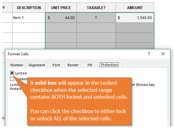
You can click the checkbox to lock or unlock ALL cells in the selected range.
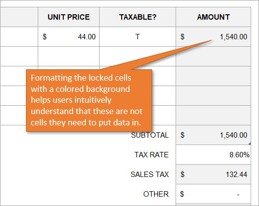
3. Use different formatting for locked cells
By changing the formatting of cells that are locked, you give your users a visual clue that those cells are off limits. In this example the locked cells have a gray fill color. The unlocked (editable) cells are white. You can also provide a guide on the sheet or instructions tab.
You might be wondering where I found this template for a quote. I got it from the template library. You can access the library by going to the File tab, choosing New, and using the search word “quote.”
You can find all sorts of useful templates there, including invoices, calendars, to-do lists, budgets, and more.
Conclusion
By locking your cells and protecting your sheet, you can keep your formulas safe from tampering by other users, and prevent mistakes.
I hope this simple tutorial proves helpful to you. Please leave a comment below if you have any tips or questions about locking cells, protecting sheets with passwords, or preventing users from changing cells.
Thank you! 🙂