
SEARCH, SEARCHB functions
Excel for Microsoft 365 Excel for Microsoft 365 for Mac Excel for the web Excel 2021 Excel 2021 for Mac Excel 2019 Excel 2019 for Mac Excel 2016 Excel 2016 for Mac Excel 2013 Excel 2010 Excel 2007 Excel for Mac 2011 Excel Starter 2010 More…Less
This article describes the formula syntax and usage of the SEARCH and SEARCHB functions in Microsoft Excel.
Description
The SEARCH and SEARCHB functions locate one text string within a second text string, and return the number of the starting position of the first text string from the first character of the second text string. For example, to find the position of the letter «n» in the word «printer», you can use the following function:
=SEARCH(«n»,»printer»)
This function returns 4 because «n» is the fourth character in the word «printer.»
You can also search for words within other words. For example, the function
=SEARCH(«base»,»database»)
returns 5, because the word «base» begins at the fifth character of the word «database». You can use the SEARCH and SEARCHB functions to determine the location of a character or text string within another text string, and then use the MID and MIDB functions to return the text, or use the REPLACE and REPLACEB functions to change the text. These functions are demonstrated in Example 1 in this article.
Important:
-
These functions may not be available in all languages.
-
SEARCHB counts 2 bytes per character only when a DBCS language is set as the default language. Otherwise SEARCHB behaves the same as SEARCH, counting 1 byte per character.
The languages that support DBCS include Japanese, Chinese (Simplified), Chinese (Traditional), and Korean.
Syntax
SEARCH(find_text,within_text,[start_num])
SEARCHB(find_text,within_text,[start_num])
The SEARCH and SEARCHB functions have the following arguments:
-
find_text Required. The text that you want to find.
-
within_text Required. The text in which you want to search for the value of the find_text argument.
-
start_num Optional. The character number in the within_text argument at which you want to start searching.
Remark
-
The SEARCH and SEARCHB functions are not case sensitive. If you want to do a case sensitive search, you can use FIND and FINDB.
-
You can use the wildcard characters — the question mark (?) and asterisk (*) — in the find_text argument. A question mark matches any single character; an asterisk matches any sequence of characters. If you want to find an actual question mark or asterisk, type a tilde (~) before the character.
-
If the value of find_text is not found, the #VALUE! error value is returned.
-
If the start_num argument is omitted, it is assumed to be 1.
-
If start_num is not greater than 0 (zero) or is greater than the length of the within_text argument, the #VALUE! error value is returned.
-
Use start_num to skip a specified number of characters. Using the SEARCH function as an example, suppose you are working with the text string «AYF0093.YoungMensApparel». To find the position of the first «Y» in the descriptive part of the text string, set start_num equal to 8 so that the serial number portion of the text (in this case, «AYF0093») is not searched. The SEARCH function starts the search operation at the eighth character position, finds the character that is specified in the find_text argument at the next position, and returns the number 9. The SEARCH function always returns the number of characters from the start of the within_text argument, counting the characters you skip if the start_num argument is greater than 1.
Examples
Copy the example data in the following table, and paste it in cell A1 of a new Excel worksheet. For formulas to show results, select them, press F2, and then press Enter. If you need to, you can adjust the column widths to see all the data.
|
Data |
||
|---|---|---|
|
Statements |
||
|
Profit Margin |
||
|
margin |
||
|
The «boss» is here. |
||
|
Formula |
Description |
Result |
|
=SEARCH(«e»,A2,6) |
Position of the first «e» in the string in cell A2, starting at the sixth position. |
7 |
|
=SEARCH(A4,A3) |
Position of «margin» (string for which to search is cell A4) in «Profit Margin» (cell in which to search is A3). |
8 |
|
=REPLACE(A3,SEARCH(A4,A3),6,»Amount») |
Replaces «Margin» with «Amount» by first searching for the position of «Margin» in cell A3, and then replacing that character and the next five characters with the string «Amount.» |
Profit Amount |
|
=MID(A3,SEARCH(» «,A3)+1,4) |
Returns the first four characters that follow the first space character in «Profit Margin» (cell A3). |
Marg |
|
=SEARCH(«»»»,A5) |
Position of the first double quotation mark («) in cell A5. |
5 |
|
=MID(A5,SEARCH(«»»»,A5)+1,SEARCH(«»»»,A5,SEARCH(«»»»,A5)+1)-SEARCH(«»»»,A5)-1) |
Returns only the text enclosed in the double quotation marks in cell A5. |
boss |
Need more help?
How to Use Excel’s MATCH Function to Find a Value
Locate the position of a specific value in your data set
Updated on November 15, 2019
- The MATCH function syntax is =MATCH(Lookup_value,Lookup_array,Match_type).
- Can be entered manually. Or, to use Excel’s built-in functions, select Formulas > Lookup & Reference > MATCH.
- Returns a number that indicates the first relative position of data in a list, array, or selected range of cells.
Here’s how to use Excel’s MATCH function to locate the position of a value in a row, column, or table. This is helpful when you must find the item’s place in the list instead of the item itself.
MATCH Function Syntax
A function’s syntax refers to the layout of the function and includes the function’s name, brackets, comma separators, and arguments. The syntax for the MATCH function is:
=MATCH(Lookup_value,Lookup_array,Match_type)
MATCH Function Arguments
Any input you give to a function is called an argument. Most of the functions found in Excel require some input or information in order to calculate correctly.
These are the MATCH function’s arguments:
Lookup_value
Lookup_value (required) is the value that you want to find in the list of data. This argument can be a number, text, logical value, or a cell reference.
Lookup_array
Lookup_array (required) is the range of cells being searched.
Match_type
Match_type (optional) tells Excel how to match the Lookup_value with values in the Lookup_array. The default value for this argument is 1. The choices are -1, 0, or 1.
- If Match_type equals 1 or is omitted, MATCH finds the largest value that is less than or equal to the Lookup_value. The Lookup_array data must be sorted in ascending order.
- If Match_type equals 0, MATCH finds the first value that is exactly equal to the Lookup_value. The Lookup_array data can be sorted in any order.
- If Match_type equals -1, MATCH finds the smallest value that is greater than or equal to the Lookup_value. The Lookup_array data must be sorted in descending order.
The MATCH example shown in this tutorial uses the function to find the position of the term Gizmos in an inventory list. The function syntax can be entered manually into a cell or by using Excel’s built-in functions, as shown here.
To enter the MATCH function and arguments:
-
Open a blank Excel worksheet and enter the data in columns C, D, and E, as shown in the image below. Leave cell D2 blank, as that particular cell will host the function.
-
Select cell D2 to make it the active cell.
-
Select the Formulas tab of the ribbon menu.
-
Choose Lookup & Reference to open the Function drop-down list.
-
Select MATCH in the list to open the Function Arguments dialog box. (In Excel for Mac, the Formula Builder opens.)
-
Place the cursor in the Lookup_value text box.
-
Select cell C2 in the worksheet to enter the cell reference.
-
Place the cursor in the Lookup_array text box.
-
Highlight cells E2 to E7 in the worksheet to enter the range.
-
Place the cursor in the Match_type text box.
-
Enter the number 0 on this line to find an exact match to the data in cell D3.
-
Select OK to complete the function. (In Excel for Mac, select Done.)
-
The number 5 appears in cell D3 since the term Gizmos is the fifth item from the top in the inventory list.
-
When you select cell D3, the complete function appears in the formula bar above the worksheet.
=MATCH(C2,E2:E7,0)
Combine MATCH With Other Excel Functions
The MATCH function is usually used in conjunction with other lookup functions, such as VLOOKUP or INDEX and is used as input for the other function’s arguments, such as:
- The col_index_num argument for VLOOKUP.
- The row_num argument for the INDEX function.
Thanks for letting us know!
Get the Latest Tech News Delivered Every Day
Subscribe
The FIND function is a built-in Worksheet Function (WS) in Microsoft Excel, which you can use to locate a sub-string or a specific character’s position within a text string. It is categorized as a TEXT function in Excel.
If the FIND function fails to find the text, it will return a #VALUE error. Note that the Excel FIND function will perform a case-sensitive search.
Excel FIND function is commonly used by financial analysts for locating specific data or text occurrences in a cell.

Syntax of Excel FIND function
=FIND(find_text, within_text, [start_num])
Arguments:
'find_text' – The text/sub-string you want to locate.'within_text' – This argument is the string within which you wish to perform the search. You can supply a cell reference or type in the string into the formula.'start_num' – This is an optional argument wherein you specify the character from which your search must begin. If you omit this argument, the function will assume this parameter as 1, i.e., the search will begin from the 1st character of the 'within_text' string.
Things to Remember
- The FIND function in Excel is case-sensitive and does not allow the usage of wildcard characters. For locating case-insensitive matches, take a look at the SEARCH function.
- The FIND function will search the
'find_text'argument in'within_text'and return the first character’s position. - You may search for either a substring or a character with the
'find_text'argument. You may use cell references or text characters for both'find_text'and'within_text'The FIND function will return ‘1’ when the'find_text'argument is an empty string «». - The FIND function returns #VALUE! error when:
- The FIND function cannot locate
'find_text'in'within_text'or - The
'start_num'argument is negative, 0, or greater than the length of'within_text'
- The FIND function cannot locate
Examples of FIND function in Excel
Example 1 – Finding a word’s position in a text string

In this example, when you search for «Dallas» and reference the cell A2, which has the text string «Dallas, USA» the function will return ‘1’. Here, 1 represents the position of the searched word’s starting point.
On account of the FIND function’s case-sensitivity, entering «dallas» as an argument will return #VALUE! error.
Example 2 – Search for a word in a text string

The 'start_num' argument lets you decide the starting position for performing the search in the text string. You will see that in the above example, the FIND function returns ‘1’ when we put 1 as the 'start_num'. Essentially, it searches for the text «Dallas» in «Dallas, USA».
When we change 'start_num' to ‘2’, it returns an error because it then searches for «Dallas» in «allas, USA».
Note that skipping the 'start_num' argument will result in the FIND function assuming ‘1’ as the starting position.
Example 3 – When the searched text occurs multiple times in a text string

Since the FIND function refers to the 'start_num' argument to see if you would like to define a starting position, it returns ‘1’ when you input 'start_num' as 1. This is because it finds «Dallas» at position ‘1’ in «Dallas, Dallas, USA».
When you input 'start_num' as 2, though, you will see that it returns ‘9’. What is happening here is that the FIND function tries to look for the word «Dallas» in «allas, Dallas, USA» since you are asking the function to start searching from the second position. Here, 9 is the starting position of the 2nd «Dallas» in «Dallas, Dallas, USA».
Example 4 – Look for a specific character’s Nth occurrence in a string.

Let’s now assume that you would like to know the position of the second «,» in the list that has the format «City, Country, Continent».
For this, we will need to nest two FIND functions one within another. The second FIND function will go in the first FIND function as a third argument ('start_num'), like so:
=FIND(",",A2,FIND(",",A2)+1)
With the third argument, you are instructing the first FIND function to start searching for «,» exactly after the first occurrence of a «,» in the string.
Pro tip: You can use the CHAR and SUBSTITUTE functions to do this more simply, with the following formula:
=FIND(CHAR(1), SUBSTITUTE(A5,",",CHAR(1),2)
Example 5 – Retrieving the first part of a text string separated by «,» (comma)

Let’s assume you want the list of just the name of cities, without the name of the country, i.e., the characters right before «,»).
To accomplish this, we will use the LEFT function and the FIND function together. The FIND function will give us the position of «,» and the LEFT function will allow us to retrieve the name of the cities.
In our example, the FIND function will return 10 when executed on «Amsterdam, Netherlands». From this, we will subtract 1 since we don’t want to include the «,» in our output.
Next, we embed a FIND function into the LEFT function and use FIND(",", A2,1)-1 as the second argument, like so:
=LEFT(A2,FIND(",",A2,1)-1)
Example 6 – Retrieving the second part of a text string separated by «,» (comma)

Let’s take example 5, and try to retrieve the second part of the string.
To accomplish this, we will use the MID function and the FIND function together. The FIND function will give us the position of «,» and the MID function will allow us to fetch the specific string portion that we need.
In our example, the FIND function will return 10 when executed on «Amsterdam, Netherlands». From this, we will add 1 since we don’t want to include the «,» in our output.
Next, we use a MID function and pass the FIND function to it FIND(",", A2,1)+1 as the second argument, like so:
=MID(A2,FIND(",",A2,1)+1,100)
FIND function vs. SEARCH function in Excel
Both Find and Search functions have a similar syntax and application. However, there are 2 differences between these functions. Let’s dive into what these differences are:
1. Acceptance of wildcard characters
Unlike with the FIND function, you may use wildcard characters in the SEARCH function’s 'find_text' argument.
To match one character – we will use a question mark ‘?’, and to match a series of characters – we will use an asterisk mark ‘*’.
Let’s work this out with an example:

We will use the syntax:
=SEARCH(",*EUROPE",A2)
Notice how the Excel SEARCH function returns the first character’s position if you input both «,» and the «continent name» regardless of how many characters exist between the text string referred to in the 'within_text'argument.
Pro tip: For finding a ‘?’ or ‘*’, just add a tilde (~) in front of the question mark or the asterisk.
2. FIND is case-sensitive, while SEARCH is case-insensitive
As I mentioned previously, case-sensitivity is another differentiating factor between the two functions.

In our example, when using the FIND function to search for ‘A’ it returns the position of the capital A in ‘USA’. However, searching for ‘A’ with the SEARCH function returns the position of the ‘a’ in ‘Dallas’ because it is case-insensitive.
Handling #VALUE! errors in the FIND function
To deal with #VALUE! errors, we can use the IFERROR function.
Let’s revisit our first example where we first encountered a #VALUE! error with FIND function on account of the FIND function’s case-sensitivity.

Here is the syntax we will use to fix this:
=IFERROR(FIND("dallas",A3,1), "Not Found!")
Using this syntax, we will «trap» the error and replace it with a standard string in the second argument of the IFERROR function, which in our case is «Not Found!». So, until the FIND function is able to return a matched string, the function will keep returning «Not Found».
Excel FIND Function (Example + Video)
When to use Excel FIND Function
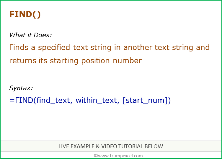
Excel FIND function can be used when you want to locate a text string within another text string and find its position.
What it Returns
It returns a number that represents the starting position of the string you are finding in another string.
Syntax
=FIND(find_text, within_text, [start_num])
Input Arguments
- find_text – the text or string that you need to find.
- within_text – the text within which you want to find the find_text argument.
- [start_num] – a number that represents the position from which you want the search to begin. If you omit it, it starts from the beginning.
Additional Notes
- If the start number is not specified, then it starts looking from the beginning of the string.
- Excel FIND function is case-sensitive. If you want to do a case-insensitive search, use Excel SEARCH function.
- Excel FIND function cannot handle wildcard characters. If you want to use wildcard characters, use the Excel SEARCH function.
- It returns a #VALUE! error if the searched string is not found in the text.
Excel FIND Function – Examples
Here are four examples of using Excel FIND function:
Searching for a Word in a Text String (from the beginning)
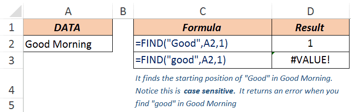
In the above example, when you look for the word Good in the text Good Morning, it returns 1, which is the position of the starting point of the searched word.
Note that Excel FIND function is case-sensitive. When you use good instead of Good, it returns a #VALUE! error.
If you are looking for a case-insensitive search, use Excel SEARCH function.
Finding a Word in a Text String (with a specified beginning)
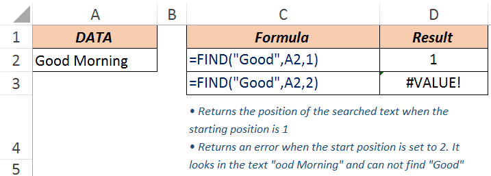
The third argument in the FIND function is the position within the text from where you want to start the search. In the example above, the function returns 1 when you search for the text Good in Good Morning and the starting position is 1.
However, it returns an error when you make it start at 2. Hence, it looks for the text Good in ood Morning. Since it can not find it, it returns an error.
Note: If you skip the last argument and don’t provide the starting position, by default it takes it as 1.
When there are Multiple Occurrence of the Searched Text
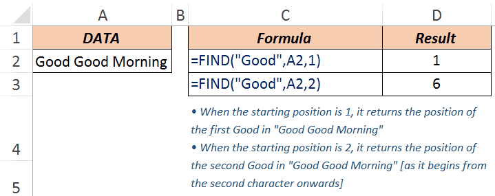
Excel FIND function starts looking in the specified text from the specified position. In the above example, when you look for the text Good in Good Good Morning with the starting position as 1, it returns 1, as it finds it at the beginning.
When you start the search from the second character onwards, it returns 6, as it finds the matching text at the sixth position.
Extracting Everything to the Left a Specified Character/String
Suppose you have the email ids do some superheroes as shown below and you want to extract only the username part (which would be the characters before the @).
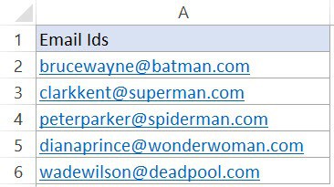
Below is the formula that will find the position of ‘@’ in each email id and extract all the characters to the left of it:
=LEFT(A2,FIND(“@”,A2,1)-1)

The FIND function in this formula gives the position of the ‘@’ character. The LEFT function that uses this position to extract the username.
For example, in the case of brucewayne@batman.com, the FIND function returns 11. LEFT function then uses FIND(“@”,A2,1)-1 as the second argument to get the username.
Note that 1 is subtracted from the value returned by the FIND function as we want to exclude the @ from the result of the LEFT function.
Excel FIND Function – VIDEO
Related Excel Functions:
- Excel LOWER Function.
- Excel UPPER Function.
- Excel PROPER Function.
- Excel REPLACE Function.
- Excel SEARCH Function.
- Excel SUBSTITUTE Function.
You May Also Like the Following Tutorials:
- How to Quickly Find and Remove Hyperlinks in Excel.
- How to Find Merged Cells in Excel.
- How to Find and Remove Duplicates in Excel.
- Using Find and Replace in Excel.
Top 10 TEXTS Functions in Excel
Transforming and cleaning text is an essential for any analyst, teacher or secretary. Luckily Excel provides a quick and easy ways to transform text in a spreadsheet using using native functions. Check out the
Excel Text Function Training Video
- FIND:
Definition: The FIND function is used in Excel to locate the position of the required text string within the another available text string
Arguments/Syntax: FIND(find_text, within_text, [start_num])
find_text: It is required argument. It takes the text user wants to find
within_text: It is required argument. The text containing the text user wants to find
start_num: It is optional argument. It specifies the character at which to start the search. By default, it takes the value 1.
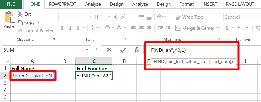
Example: Suppose, in Excel the cell A2 contains a full name of a person as “Roland Watson”. Now, if user wants to find the position of text “an” within the name of the person, then FIND functions can be used; for example, FIND(“an”,”Roland Watson” ,1). The output of this function is 4 as the starting position text “an” is 4 within ”Roland Watson”.
- LEFT:
Definition: LEFT function in Excel returns the left hand side characters from a text string based on the number of characters specified by the user.
Arguments/Syntax: LEFT(text, [num_chars])
text: It is required argument. It is the text string that contains the characters user wants to extract
num_chars: It is optional argument. It specifies the number of characters user wants to extract from left side. By default it takes the value 1.
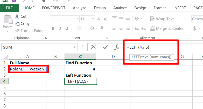
Example: Suppose, in Excel the cell A2 contains a full name of a person as “Roland Watson”. Now, if user wants to extract the first 5 letters of the name then LEFT functions can be used; for example, LEFT(”Roland Watson” ,5). The output of this function is “Rolan”.
- RIGHT:
Definition: RIGHT function in excel returns the right hand side characters from a text string based on the number of characters specified by the user.
Arguments/Syntax: RIGHT(text, [num_chars])
text: It is required argument. It is the text string that contains the characters user wants to extract
num_chars: It is optional argument. It specifies the number of characters user wants to extract from right side. By default it takes the value 1.
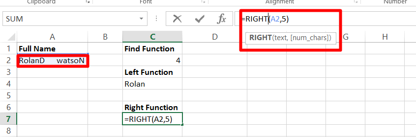
Example: Suppose, in Excel the cell A2 contains a full name of a person as “Roland Watson”. Now, if user wants to extract the last 5 letters of the name then RIGHT function can be used; for example, RIGHT(”Roland Watson” ,5). The output of this function is “atson”.
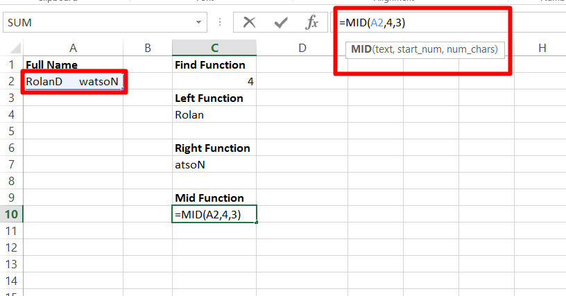
- MID:
Definition: MID function in Excel returns the number of characters from a text string based on the starting position and number of characters specified by the user.
Arguments/Syntax: MID(text, start_num, num_chars)
text: It is required argument. It is the text string that contains the characters user wants to extract
start_num: It is required argument. It specifies the character at which to start the extract.
num_chars: It is required argument. It specifies the number of characters user wants to extract from the start position
Example: Suppose, in Excel the cell A2 contains a full name of a person as “Roland Watson”. Now, if user wants to extract the “and” text from the name then MID function can be used; for example, MID(”Roland Watson”,4,3). The output of this function is “and”.
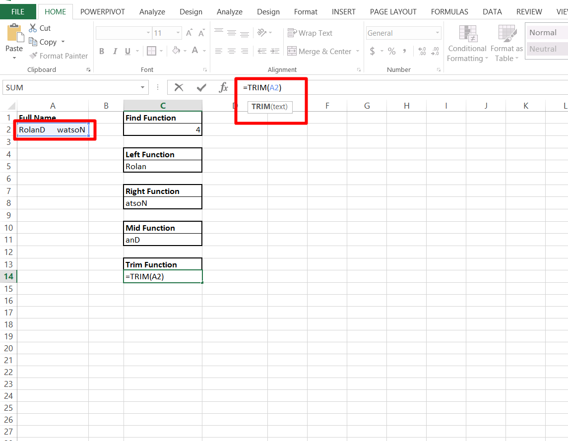
- TRIM:
Definition: TRIM function in Excel remove all the extra spaces from the text except for the single spaces between the words. It is used when the text has irregular spacing between words.
Arguments/Syntax: TRIM(text)
text: It is required argument. It is the text string that contains the irregular spacing between the words
Example: Suppose, in Excel the cell A2 contains a full name of a person as “Roland Watson”. But in between the first name (“Roland”) and last name (“Watson”) there are two blank spaces. Now, if user wants to remove the extra blank spaces then TRIM function can be used; for example, TRIM(”Roland Watson”). The output of this function is “Roland Watson”.
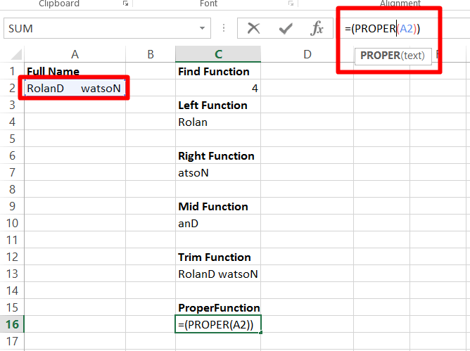
- PROPER:
Definition: PROPER function in Excel capitalizes the first letter of each of the words in the string and converts all the other letters of the words to lower case.
Arguments/Syntax: PROPER(text)
text: It is required argument. It takes the text string that user wants to partially capitalize.
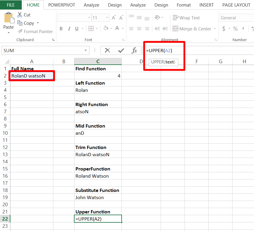
Example: Suppose, in Excel the cell A2 contains a full name of a person as “RolAnD WatsON”. Now, if user wants to make the name in proper way then PROPER function can be used; for example, PROPER(”RolAnD WatsON”). The output of this function is “Roland Watson”.
- SUBSTITUTE:
Definition: SUBSTITUTE function in Excel is used to replace the any part of the old text string with the new text string.
Arguments/Syntax: SUBSTITUTE (text,old_text,new_text,[instance_num])
text: It is required argument. The text containing text for which user wants to substitute characters.
old_text: It is required argument. It is the text user wants to replace
new_text: It is required argument. It is the text user wants to replace the old text with
[instance_num]: It is optional argument. Specifies which occurrence of old_text user wants to replace with new_text. If user specify instance_num, only that instance of old_text is replaced. Otherwise, every occurrence of old_text in text is changed to new_text.
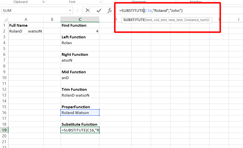
Example: Suppose, in Excel the cell A2 contains a full name of a person as “Roland Watson”. Now, if user wants to substitute “Roland” to “John” then SUBSTITUE function can be used; for example, SUBSTITUTE(“Roland Watson”,”Roland”,”John”). The output of this function is “John Watson”.
- UPPER:
Definition: UPPER function in excel capitalizes all the letter of each of the words in the string Arguments/Syntax: UPPER(text)
text: It is required argument. It takes the text string that user wants to capitalize completely.
Example: Suppose, in excel the cell A2 contains a full name of a person as “RolAnD WatsON”. Now, if user wants to convert the name in full capital letters then UPPER function can be used; for example, UPPER(”RolAnD WatsON”). The output of this function is “ROLAND WATSON”
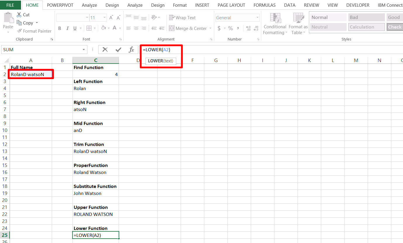
- LOWER:
Definition: LOWER function in Excel converts all the letter of each of the words in the string in small letters
Arguments/Syntax: LOWER(text)
text: It is required argument. It takes the text string that user wants to convert into small letters completely.
Example: Suppose, in Excel the cell A2 contains a full name of a person as “RolAnD WatsON”. Now, if user wants to convert the name in small letters completely then LOWER function can be used; for example, LOWER(”RolAnD WatsON”). The output of this function is “roland watson”
- REPT:
Definition: REPT function in Excel repeats the mentioned text by given number of times. REPT function can be used to fill a cell with a number of instances of a text string
Arguments/Syntax: REPT(text, number_times)
text: It is required argument. It takes the text string that user wants to repeat mutilple times
number_times: It is required argument. It takes a positive number specifying the number of times to repeat text
Example: REPT(“-“,5) = “—–“ Displays a dash (-) 5 times