
Excel for Microsoft 365 Excel for Microsoft 365 for Mac Excel for the web Excel 2021 Excel 2021 for Mac Excel 2019 Excel 2019 for Mac Excel 2016 Excel 2016 for Mac Excel 2013 Excel 2010 Excel for Mac 2011 Excel Mobile More…Less
Managing personal finances can be a challenge, especially when trying to plan your payments and savings. Excel formulas and budgeting templates can help you calculate the future value of your debts and investments, making it easier to figure out how long it will take for you to reach your goals. Use the following functions:
-
PMT calculates the payment for a loan based on constant payments and a constant interest rate.
-
NPER calculates the number of payment periods for an investment based on regular, constant payments and a constant interest rate.
-
PV returns the present value of an investment. The present value is the total amount that a series of future payments is worth now.
-
FV returns the future value of an investment based on periodic, constant payments and a constant interest rate.
Figure out the monthly payments to pay off a credit card debt
Assume that the balance due is $5,400 at a 17% annual interest rate. Nothing else will be purchased on the card while the debt is being paid off.
Using the function PMT(rate,NPER,PV)
=PMT(17%/12,2*12,5400)
the result is a monthly payment of $266.99 to pay the debt off in two years.
-
The rate argument is the interest rate per period for the loan. For example, in this formula the 17% annual interest rate is divided by 12, the number of months in a year.
-
The NPER argument of 2*12 is the total number of payment periods for the loan.
-
The PV or present value argument is 5400.
Figure out monthly mortgage payments
Imagine a $180,000 home at 5% interest, with a 30-year mortgage.
Using the function PMT(rate,NPER,PV)
=PMT(5%/12,30*12,180000)
the result is a monthly payment (not including insurance and taxes) of $966.28.
-
The rate argument is 5% divided by the 12 months in a year.
-
The NPER argument is 30*12 for a 30 year mortgage with 12 monthly payments made each year.
-
The PV argument is 180000 (the present value of the loan).
Find out how to save each month for a dream vacation
You’d like to save for a vacation three years from now that will cost $8,500. The annual interest rate for saving is 1.5%.
Using the function PMT(rate,NPER,PV,FV)
=PMT(1.5%/12,3*12,0,8500)
to save $8,500 in three years would require a savings of $230.99 each month for three years.
-
The rate argument is 1.5% divided by 12, the number of months in a year.
-
The NPER argument is 3*12 for twelve monthly payments over three years.
-
The PV (present value) is 0 because the account is starting from zero.
-
The FV (future value) that you want to save is $8,500.
Now imagine that you are saving for an $8,500 vacation over three years, and wonder how much you would need to deposit in your account to keep monthly savings at $175.00 per month. The PV function will calculate how much of a starting deposit will yield a future value.
Using the function PV(rate,NPER,PMT,FV)
=PV(1.5%/12,3*12,-175,8500)
an initial deposit of $1,969.62 would be required in order to be able to pay $175.00 per month and end up with $8500 in three years.
-
The rate argument is 1.5%/12.
-
The NPER argument is 3*12 (or twelve monthly payments for three years).
-
The PMT is -175 (you would pay $175 per month).
-
The FV (future value) is 8500.
Find out how long it will take to pay off a personal loan
Imagine that you have a $2,500 personal loan, and have agreed to pay $150 a month at 3% annual interest.
Using the function NPER(rate,PMT,PV)
=NPER(3%/12,-150,2500)
it would take 17 months and some days to pay off the loan.
-
The rate argument is 3%/12 monthly payments per year.
-
The PMT argument is -150.
-
The PV (present value) argument is 2500.
Figure out a down payment
Say that you’d like to buy a $19,000 car at a 2.9% interest rate over three years. You want to keep the monthly payments at $350 a month, so you need to figure out your down payment. In this formula the result of the PV function is the loan amount, which is then subtracted from the purchase price to get the down payment.
Using the function PV(rate,NPER,PMT)
=19000-PV(2.9%/12, 3*12,-350)
the down payment required would be $6,946.48
-
The $19,000 purchase price is listed first in the formula. The result of the PV function will be subtracted from the purchase price.
-
The rate argument is 2.9% divided by 12.
-
The NPER argument is 3*12 (or twelve monthly payments over three years).
-
The PMT is -350 (you would pay $350 per month).
See how much your savings will add up to over time
Starting with $500 in your account, how much will you have in 10 months if you deposit $200 a month at 1.5% interest?
Using the function FV(rate,NPER,PMT,PV)
=FV(1.5%/12,10,-200,-500)
in 10 months you would have $2,517.57 in savings.
-
The rate argument is 1.5%/12.
-
The NPER argument is 10 (months).
-
The PMT argument is -200.
-
The PV (present value) argument is -500.
See also
PMT function
NPER function
PV function
FV function
Need more help?
Want more options?
Explore subscription benefits, browse training courses, learn how to secure your device, and more.
Communities help you ask and answer questions, give feedback, and hear from experts with rich knowledge.
Excel — is the versatile analytical and computational tool that is often used by lenders (banks, investors, etc.) and borrowers (businessmen, companies, private persons, etc.).
Quickly navigate in the intricate formulas, calculate to interest, payouts, overpayment to allow Microsoft Excel program functions.
How to calculate credit payments in Excel
Monthly payments depend on the loan repayment scheme. There are annuity and differentiated payments:
- The annuity assumes that the client makes each month the same amount.
- When the differentiated scheme of repayment of debt before the financial organization interest is charged on the balance of the loan amount. Therefore, the monthly payments will be reduced.
Increasingly used annuity: it`s more profitable for the bank, and it is more convenient for the majority of customers.
The calculation of annuity payments on the loan in Excel
The monthly annuity payment is calculated as follows:
S = C * V
where:
- S – sum, is the payment amount on the loan;
- C – coefficient, is the annuity payment rate;
- V – is the value of the loan.
The annuity factor Formula:
С = (i * (1 + i) ^ n) / ((1 + i) ^ n-1)
- where is i – the interest rate for the month, the result of dividing the annual rate by 12;
- n – is the loan term in months.
There is a special feature in Excel which said to the annuity payments. This is: =PMT().
- Fill in the input data for calculating the monthly payments on the credit. This is loan amount, interest and term.
- To make the repayment schedule. It`s empty till.
- In the first cell of the column «Credit payments», introduced the formula of the calculating the loan annuity payments in Excel: =PMT($B$3/12,$B$4,$B$2). To fix the cells, are used to the absolute links. In the formula may be administered directly to the numbers and not the reference cell data. Then it will have the following form: =PMT(18%/12,36,100000).
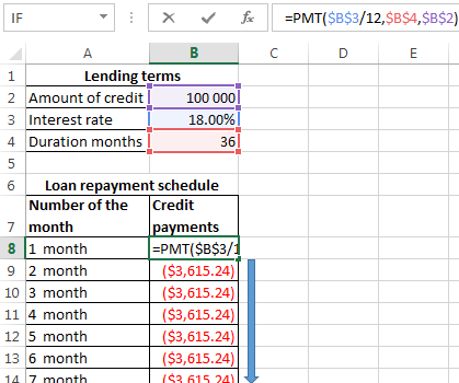
The cells turned into red, because we’ll give these money to the bank and to lose the money.
The calculation of payments in Excel for the differentiated scheme of repayment
The differentiated payment method implies that:
- the principal amount is distributed over the period of payment in the equal installments;
- the loan interest accrued on the balance.
The formula for the calculating to the differential payment:
DP = NEO / (PP + PS * NEO)
where:
- DP – is the monthly payment on the loan;
- NEO – is the loan balance;
- PP – the number of remaining until the end of the repayment period;
- PS – is the interest rate per month (the annual rate divided by 12).
Draw up the schedule for repayment of the previous loan on the differentiated scheme.
The input dates are the same:
| Lending terms | |
| Amount of credit | $100 000 |
| Interest rate | 18% |
| Duration months | 36 |
To make the schedule of repayment of the loan:
| Number of the month | Balance receivable on the loan | Payment of interest | Payment of principal | Final payment |
| 1 month |
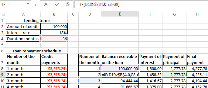
Balance receivable on the loan: in the first month it is equal to the entire amount =$B$2. In the second one and in the subsequent ones — calculated by the formula: =IF(D10>$B$4,0,E8-G9). Where is:
- D10 – the number of the current period;
- $B$4 – is the term of the loan;
- E8 – is the balance of the loan in the previous period;
- G9 — is the principal debt in the previous period.
Payment of interest: the balance of the loan in the current period multiplied by the monthly interest rate / 12 months: =E9*($B$3/12).
Payment of principal: the amount of the loan divided by the period: =IF(D9<=$B$4,$B$2/$B$4,0).
Final payment: the sum of «the interest» and «the main debt» in the current period: =F8+G8.
We substitute to the formulas in the corresponding columns. Copy them to the entire table.
To compare the overpayment on the annuity and the differentiated scheme of the repayment on credit:
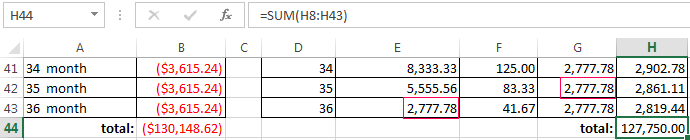
The red figure – is the annuity (was taken 100 000 rubles), the black one – is the differentiated way.
Interest calculation formula for loans in Excel
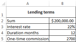
The calculation of interest on the loan in Excel and calculate the effective interest rate, with the following information on the bank offers credit:
We carry out interest calculation on loan and calculate the effective interest rate with the following information on the bank offers credit.
Fill in the table type:
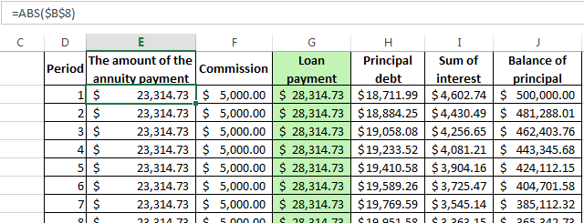
The commission is taken monthly from the whole sum. The total loan payment — this is the annuity payment plus the commission. The sum of the main debt and the sum of interest – there are components parts of the annuity payment.
The principal amount = the annuity payment – the interest.
The sum of interest = the remaining debt * the monthly interest rate.
The balance of principal = the residue of the previous period – the sum of the principal debt in the previous period.
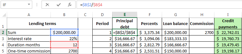
Based on the table of monthly payments, calculate the effective interest rate:
- took the credit 500 000 rubles;
- returned to the bank — 684 881. 67 rubles (the sum of all payments on the loan);
- the overpayment was 184 881. 67 rubles;
- the interest rate — 184 881 67/500 000 * 100, or 37%.
- the harmless commission of 1% was cost for the borrower so expensive.
The effective interest rate of the loan without the commission will be 13%. The counting is carried out in the same way.
The calculation of effective interest rate in Excel
According to the law about the consumer credit for the calculation of the effective interest rate now is applied the new formula. EIR (Effective Interest Rate) is defined in percentage of up to the third decimal place according to the following formula:
- EIR = i * CHBP * 100;
- where is i — the interest rate of the base period;
- NBP — the number of base periods in a calendar year.
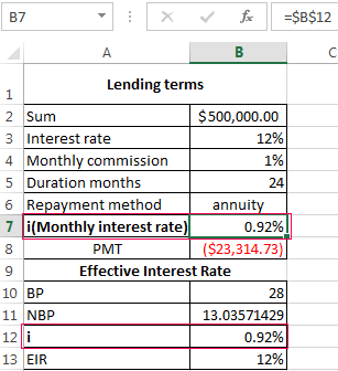
Take for example the following dates on the loan:
For calculating of the effective interest rate is necessary to make a payment schedule (see the order above).
It is necessary to determine the base period (BP). The law states that this is the standard time interval, which is found in most of the repayment schedule. Example BP = 28 days.
Then we find NBP: 365/28 = 13.
Now you can find the interest rate of the base period:
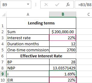
We have all the necessary dates — substitute them in the EIR formula: =B9*B8
To obtain the percentages in Excel, you do not need to multiple by 100. It is enough to set for the cell with the result to the percentage format.
EIR for the new formula is coincided with the annual interest rate on the loan.
Download credit calculator in Excel
Thus, for calculating the annuity payments on the loan is used the simplest function PLT. As you can see, the differentiated way of repayment is a bit more complicated.
Return to Excel Formulas List
Download Example Workbook
Download the example workbook
This tutorial will demonstrate how to calculate monthly loan payments in Excel and Google Sheets.
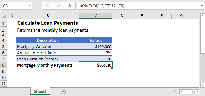
Calculate Loan Payments
Calculating loan payments is easy, whether it’s for mortgages, cars, students, or credit cards. First you need to know the type of loan before you can calculate the payments.
Interest-Only Loan Payment
An interest-only loan is the one in which the borrower pays only the interest for a certain period of time.
These types of loan’s monthly payments can be calculated by multiplying the interest rate of the loan with the loan amount and dividing it by 12.
=(loan_amount*interest_rate)/12Interest-only Mortgage Payment Calculation
=(C3*C4)/C5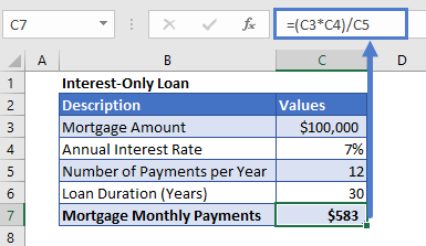
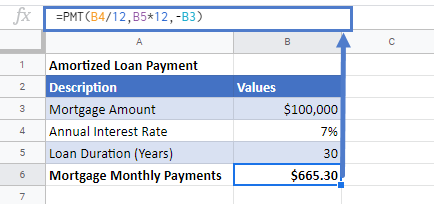
Amortized Loan Payment
An amortized loan is a type of loan for which the loan amount plus the interest owed is paid off over a set period of regular payments.
The general formula to calculate payment from this type of loan is
=loan_amount/[{((1+interest_rate)^number_of_payments)-1}/{interest_rate(1+interest_rate)^number_of_payments}]The above formula is kind of a complex one.
Thankfully, Excel has made it easy for you to calculate loan payments for any type of loan or credit card. Excel has a built-in function, PMT, that calculates the monthly loan payments for you. All you have to do is enter the details of the loan like the interest rate, the duration, and the principal of the loan and Excel will calculate the loan payments for you.
The syntax for the PMT Function is:
=PMT(rate,nper,pv,[fv],[type])Calculate Amortized Mortgage Monthly Payments
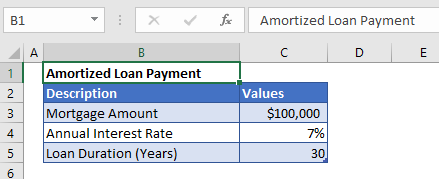
Let’s take the previous example and calculate the amortized loan payment for it.
Before applying the PMT function, we need to make sure that the interest rate and the payment period’s units are consistent.
And to do that, the annual interest rate is converted into monthly interest rate by dividing it with 12 and similarly, the payment periods are also converted into monthly payment periods by multiplying its value with 12. Also, the mortgage loan payment is entered with a negative sign in the formula,
=PMT(C4/12,C5*12,-C3)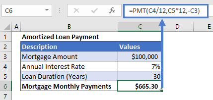
Here, we haven’t entered the fv and type arguments’ values because we don’t need them.
Calculate the loan payments in Google Sheets
The formula to calculate the loan payments works exactly the same in Google Sheets as in Excel:
Loans have four primary components: the amount, the interest rate, the number of periodic payments (the loan term) and a payment amount per period. You can use the PMT function to get the payment when you have the other 3 components.
For this example, we want to find the payment for a $5000 loan with a 4.5% interest rate, and a term of 60 months. To do this, we configure the PMT function as follows:
rate — The interest rate per period. We divide the value in C6 by 12 since 4.5% represents annual interest, and we need the periodic interest.
nper — the number of periods comes from cell C7; 60 monthly periods for a 5 year loan.
pv — the loan amount comes from C5. We use the minus operator to make this value negative, since a loan represents money owed.
With these inputs, the PMT function returns 93.215, rounded to $92.22 in the example using the currency number format.
While taking a loan from a bank or a financial institution, our primary concern is how much we have to make periodic payment (monthly, quarterly, annually) to pay back that loan on a given interest rate and in the total number of payments. Using the Excel PMT function we calculate payment for a loan based on a constant interest rate and constant payments.
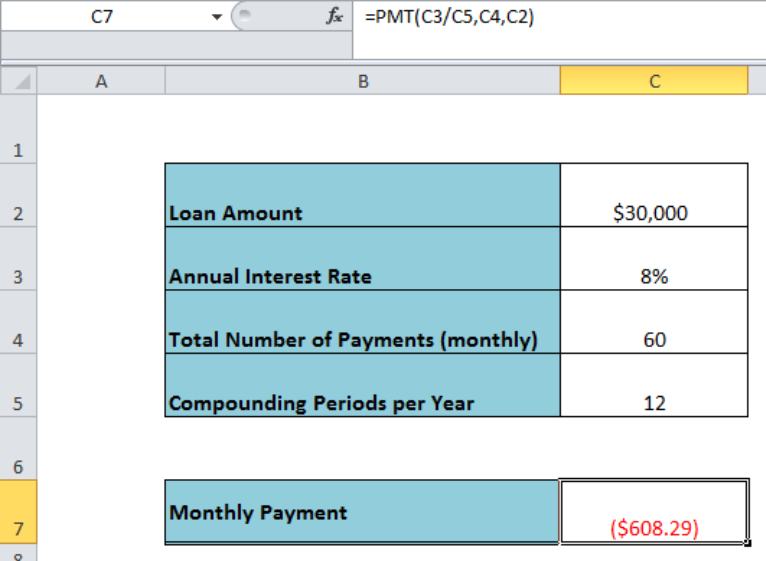 Figure 1. Calculating Payment For a Loan in Excel
Formula Syntax
The syntax for the formula to calculate payment for a loan in Excel is;
=PMT(annual rate/compounding periods, total payments, loan amount)
OR
=PMT(rate, nper, pv, [fv], [type])
Where,
- Rate (required argument): A constant interest rate
- Nper (required argument): The Total number of payments or periods
- PV (required argument): Present value or the loan amount
There are two optional arguments;
- FV (optional argument): Future value of loan amount after all payments are made. Use $0 if not known or omit this argument.
- Type (optional argument): To specify whether the payment is due at the beginning or end of the period, like at the beginning or end of the month. Use “1” for the beginning of the period and “0” for the end of the period. The default is “0”
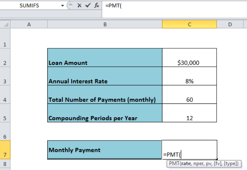 Figure 2. The Syntax of the Formula
Example
Assume we need to borrow $30,000 at 8% annual interest rate for 5 years on monthly payment terms. We can calculate the monthly payment for this loan amount using the following formula assuming the monthly payment is due at the end of the month;
=PMT(C3/C5,C4,C2)
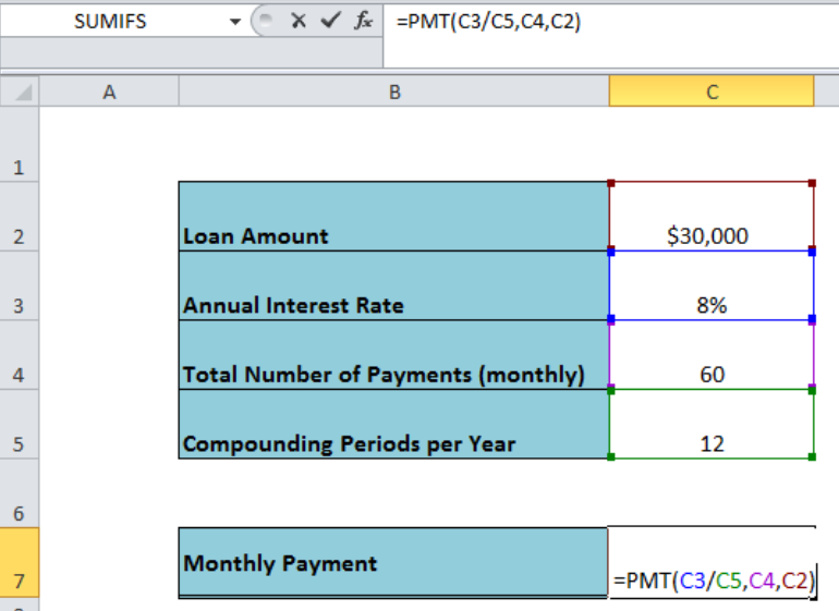 Figure 3. Using the PMT Function to Calculate Payment For a Loan
As the constant interest rate is annual, so we have to convert it into monthly interest rate by dividing it to 12 (compounding periods per year). The loan period is 5 years and payments for the loan are monthly, therefore the total number of payments would be 60 (12*5). The PMT function returns payment for the loan as a negative value to represent the cash outflow, such as;
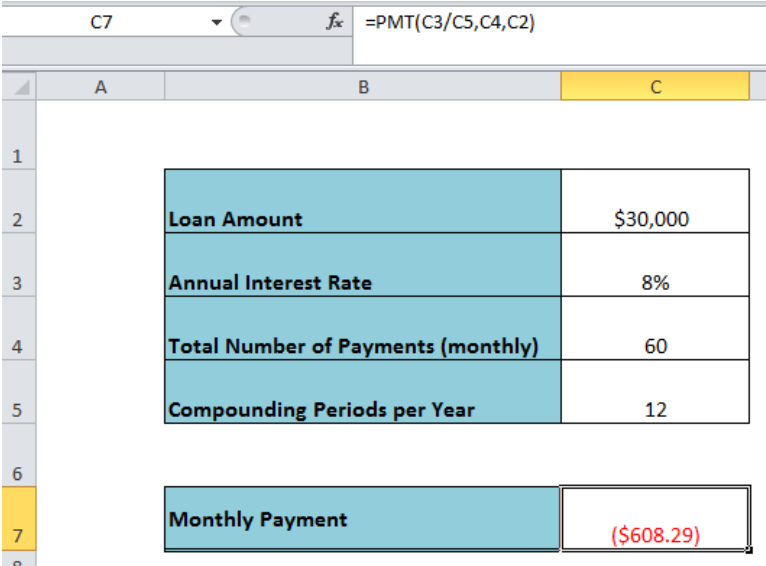 Figure 4. Final Preview of Formula to Calculate Payment For a Loan
Instant Connection to an Expert through our Excelchat Service:
Most of the time, the problem you will need to solve will be more complex than a simple application of a formula or function. If you want to save hours of research and frustration, try our live Excelchat service! Our Excel Experts are available 24/7 to answer any Excel question you may have. We guarantee a connection within 30 seconds and a customized solution within 20 minutes.