Lists of words in excel - Word и Excel - помощь в работе с программами

There should be more efficient ways to do this than my below code. It utilizes service from Dictionary.com.

You can use it as a function in worksheet, say you have «pizza» in A1, then in A2, you use =DictReference(A1) to show the definition. However I only coded it to return the first definition.

Option Explicit

Const URL_SEARCH = "http://dictionary.reference.com/browse/<WORD>?s=t"

Function DictReference(ByVal SearchWord As Variant) As String
    On Error Resume Next
    Dim sWord As String, sTxt As String
    sWord = CStr(SearchWord)
    With CreateObject("WinHttp.WinHttpRequest.5.1")
        .Open "GET", Replace(URL_SEARCH, "<WORD>", sWord), False
        .Send
        If .Status = 200 Then
            sTxt = StrConv(.ResponseBody, vbUnicode)
            ' The definition of the searched word is in div class "def-content"
            sTxt = Split(sTxt, "<div class=""def-content"">")(1)
            sTxt = Split(sTxt, "</div>")(0)
            ' Remove all unneccessary whitespaces
            sTxt = Replace(sTxt, vbLf, "")
            sTxt = Replace(sTxt, vbCr, "")
            sTxt = Replace(sTxt, vbCrLf, "")
            sTxt = Trim(sTxt)
            ' Remove any HTML codes within
            sTxt = StripHTML(sTxt)
        Else
            sTxt = "WinHttpRequest Error. Status: " & .Status
        End If
    End With
    If Err.Number <> 0 Then sTxt = "Err " & Err.Number & ":" & Err.Description
    DictReference = sTxt
End Function

Private Function StripHTML(ByVal sHTML As String) As String
    Dim sTmp As String, a As Long, b As Long
    sTmp = sHTML
    Do Until InStr(1, sTmp, "<", vbTextCompare) = 0
        a = InStr(1, sTmp, "<", vbTextCompare) - 1
        b = InStr(a, sTmp, ">", vbTextCompare) + 1
        sTmp = Left(sTmp, a) & Mid(sTmp, b)
    Loop
    StripHTML = sTmp
End Function

Источник

Last year, I wrote a post about using Excel to keep a word bank. It was one of the most popular posts of 2014 and the template was downloaded over 2000 times.

I was thrilled by the amount of people that had found it useful.

However, towards the end of 2014 I had selfishly redesigned the Word Bank for my own personal language studies because I was going back into the classroom as a student to learn more Japanese.

I wanted new features that would help keep a track of my learning. This was going to be version 2.0 of the Word Bank.

I wanted to keep a list of words I had learned, words I was still learning and words I hadn’t learned yet.
I wanted the search card to be able to look at multiple lists.
And I wanted to know approximately how many words I had learned compared to words I still had to study. (This was as much of a motivational aid to see the progress of my study.)
I also wanted to keep it in a familiar format, so I could just copy and paste words into my new file.

The version that I made back then though was more specific to learning Japanese with boxes for Romaji, Kana, and Kanji. So, I went back to version 2.0 and redesigned it so that it could be used for any language.

The result of this work is Word Bank 2.13.

This video provides a short introduction to the template.

The video run time is 2 minutes.

Contents:

Why use a word bank?
Download
Word Bank 2.1 – New Features
- The Words Sheet
- The Lists Sheet
- The Search Sheet
- The Statistics Sheet

Why use a word bank?

A word bank is a useful resource for learning and reviewing vocabulary.

A word bank can build your vocabulary by encouraging you to look for synonyms and antonyms to words you already know and you practice using them by writing example sentences.

A word bank can help motivate you to study another language by giving you a real estimation of how much new language you have actually learned during your studies.

Finally, a word bank is useful for keeping a list of situation specific language. If you are learning a language for business or travel, it’s worth while keeping a list of useful phrases that can help you communicate what you need. I do.

Why do I use an Excel file?

I used to store my vocabulary and flash cards on my old android phone, but then I changed phones and I stopped using that particular app.

I didn’t like writing down words in a notebook because it was easy to get forget which page I wrote an important word on. I also wasn’t really prepared to put the effort into making an index.

I tried keeping a list in Word. I could find words easily, but I wanted something I could sort through and only show a minimal amount of data if I chose to.

Eventually, I tried an Excel file, which does have some benefits.

You can use it completely offline. This is useful for classrooms with no, or unreliable connectivity.
It is easy to search through old entries and sort words alphabetically.
The word bank is easy to distribute. You can copy and paste vocabulary between files, e-mail the file, or store it on a cloud so it can be accessed from multiple devices.
The file size is small and if data protection is an issue the file can be password protected.

Whether your word bank is paper based or digital, any kind of word bank is useful to help you learn a language.

Top

Download

Click on Word Bank 2.13 to download the template.

After you have downloaded the template, open the Excel file.

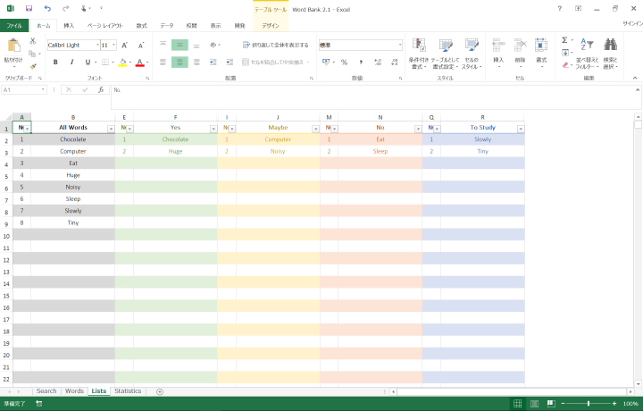
Towards the lower left-hand corner there are four tabs. Search, Words, Lists and Statistics. Click on Words.

Word Bank 2.1 – Screen capture of example entries

You will notice that there are 8 example entries on the Words sheet showing how the list is intended to be filled out.

Delete the example words and start adding your own vocabulary.

The word bank can be used as a study aid for any language.

Top

Word Bank 2.1 – New Features

I wanted to keep a list of words I had learned, words I was still learning and words I hadn’t learned yet.

Words

Word Bank 2.1 – Screen capture of the ‘Words’ sheet

The Words sheet was previously known as the Data sheet in the first version of Word Bank.

I need to categorize my entries in order to separate my master list of words into four sub lists (learned, learning, not learned, to study).

I did this by adding a drop down list to the left of the entries. When you click on a cell, a box with an arrow appears in the lower-right hand corner of the cell. Click on this arrow and a list appears. There are three words in the list: Yes, Maybe, No.

Select Yes if you feel that you have learned the word. The cell will turn green.

Select Maybe if you feel that you are still learning the word and reviewing it will be helpful. The cell will turn yellow.

Select No if you feel that you have forgotten the word or you haven’t learned it properly yet and reviewing it will be necessary. The cell will turn red.

Top

I wanted the search card to be able to look at multiple lists.

Go to the Lists sheet and you will notice that Excel will now separate those words into different color coded lists for you.

Lists

Word Bank 2.1 – Screen capture of the ‘Lists’ sheet

This sheet is protected because everything is automatically generated.

The grey column is a copy of your master list of words.

The green column lists all the words that you have learned and where you selected yes.

The yellow column lists all the words that you are still learning and where you selected maybe.

The red column lists all the words that you haven’t learned and where you selected no.

The blue column lists all the words where you haven’t yet selected a category for them. They may be future words to study.

Top

The Search sheet was previously known as the Word Card sheet in the first version of Word Bank. I had to redesign the Search sheet slightly so that it would be able to search for vocabulary from the different lists.

Click on the cell at the top of the Search sheet and a drop down list appears. Select which list you want to search from.

Select All Words and the Entry drop down list will show every word you have entered into your list.

Select New Words and the Entry drop down list will show the words you have yet to study or categorize.

Select Learned and the Entry drop down list will show the words you have marked as yes.

Select Learning and the Entry drop down list will show the words you have marked as maybe.

Select Not learned and the Entry drop down list will show the words you have marked as no.

Update: A random function has been added, so you can randomly select a word from any list to test your knowledge.

The search form changes color to match the category you have chosen.

Top

I wanted to know approximately how many words I had learned compared to words I still had to study.

The Statistics sheet has been updated to not only show the types of words you are learning, but it also displays the percentage of words you have learned. This was intended as a motivational device.

I wanted to visually show how many words I had studied compared to how many words I felt confident that I had learned. The idea being is that it would tell me if I had more words to study, more words to review or how much I had achieved.

Top

Finally a huge thanks to all the people who read the original word bank post and downloaded version 1.0. I would love to hear from you and get your feedback.

As always, if you have any questions, please leave a comment.

Alternatively you can send me a message on my Facebook page or on Twitter.

For longer messages, or for information about the technical aspects of Word Bank 2.13, you can send me a message via the contact page and I will respond to you as soon as possible.

Thanks for reading and take care!

You may also like to read:

Word Banks: Keeping track of your vocabulary – Nov. 2014. The first post I wrote about using Excel to keep vocabulary lists.

Dynamic Lists with Blank Cells, an article written by Debra Dalgleish on the Contextures blog, discusses a method that is useful for making this word bank work.

Other Excel Templates:

Creating a seating chart is easy with Excel and because it uses a dynamic list, it works in a similar way to word banks.

Источник

When we need to collect data from others, they may write different things from their perspective. Still, we need to make all the related stories under one. Also, it is common that while entering the data, they make mistakes because of typo errors. For example, assume in certain cells, if we ask users to enter either “YES” or “NO,” one will enter “Y,” someone will insert “YES” like this, and we may end up getting a different kind of results. So in such cases, creating a list of values as pre-determined values allows the users only to choose from the list instead of users entering their values. Therefore, in this article, we will show you how to create a list of values in Excel.

Create List in Excel
- #1 – Create a Drop-Down List in Excel
- #2 – Create List of Values from Cells
- #3 – Create List through Named Manager
- Things to Remember
- Recommended Articles

You can download this Create List Excel Template here – Create List Excel Template

#1 – Create a Drop-Down List in Excel

We can create a drop-down list in Excel using the “Data Validation in excelThe data validation in excel helps control the kind of input entered by a user in the worksheet.read more” tool, so as the word itself says, data will be validated even before the user decides to enter. So, all the values that need to be entered are pre-validated by creating a drop-down list in Excel. For example, assume we need to allow the user to choose only “Agree” and “Not Agree,” so we will create a list of values in the drop-down list.

In the Excel worksheet under the “Data” tab, we have an option called “Data Validation” from this again, choose “Data Validation.”

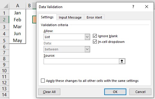
As a result, this will open the “Data Validation” tool window.

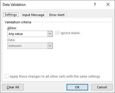
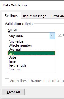
The “Settings” tab will be shown by default, and now we need to create validation criteria. Since we are creating a list of values, choose “List” as the option from the “Allow” drop-down list.

For this “List,” we can give a list of values to be validated in the following way, i.e., by directly entering the values in the “Source” list.

Enter the first value as “Agree.”

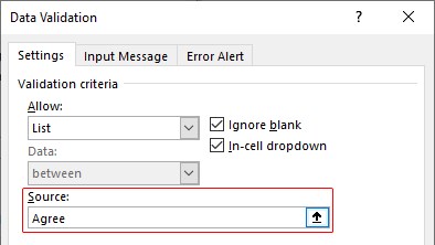
Once the first value to be validated is entered, we need to enter “comma” (,) as the list separator before entering the next value. So, enter “comma” and enter the following values as “Not Agree.”

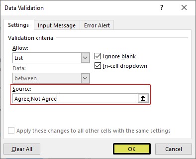
After that, click on “Ok,” and the list of values may appear in the form of the “drop-down” list.

#2 – Create a List of Values from Cells

The above method is to get started, but imagine the scenario of creating a long list of values or your list of values changing now and then. Then, it may get difficult to return and edit the list of values manually. So, by entering values in the cell, we can easily create a list of values in Excel.

Follow the steps to create a list from cell values.

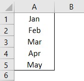
We must first insert all the values in the cells.
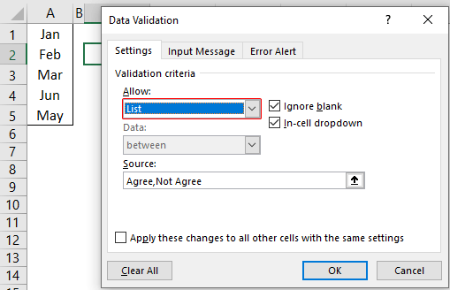
Then, open “Data Validation” and choose the validation type as “List.”
Next, in the “Source” box, we need to place the cursor and select the list of values from the range of cells A1 to A5.
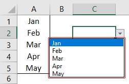
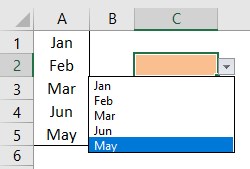
Click on “OK,” and we will have the list ready in cell C2.

So values to this list are supplied from the range of cells A1 to A5. Any changes in these referenced cells will also impact the drop-down list.

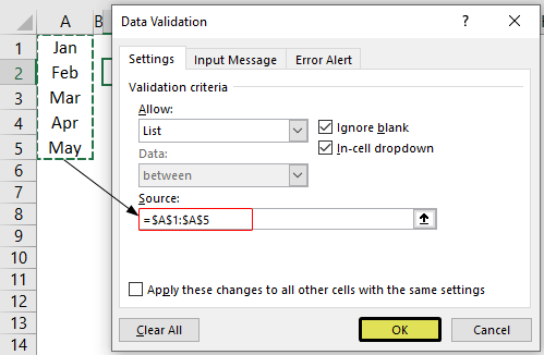
For example, in cell A4, we have a value as “Apr,” but now we will change that to “Jun” and see what happens in the drop-down list.

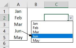
Now, look at the result of the drop-down list. Instead of “Apr,” we see “Jun” because we had given the list source as cell range, not manual entries.

#3 – Create List through Named Manager

There is another way to create a list of values, i.e., through named ranges in excelName range in Excel is a name given to a range for the future reference. To name a range, first select the range of data and then insert a table to the range, then put a name to the range from the name box on the left-hand side of the window.read more.

We have values from A1 to A5 in the above example, naming this range “Months.”

Now, select the cell where we need to create a list and open the drop-down list.

Now place the cursor in the “Source” box and press the F3 key to an open list of named ranges.

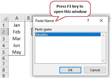
As we can see above, we have a list of names, choose the name “Months” and click on “OK” to get the name to the “Source” box.

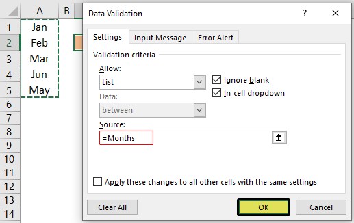
Click on “OK,” and the drop-down list is ready.

Things to Remember

The shortcut key to open data validation is “ALT + A + V + V.“
We must always create a list of values in the cells so that it may impact the drop-down list if any change happens in the referenced cells.

About This Article

Article SummaryX

1. Double-click the cell.
2. Press Alt + 7 or Option + 8 to add a bullet point.
3. Type a list item.
4. Press Alt + Enter (PC) or Control + Option + Return (Mac) to go to the next line.
5. Repeat until your list is finished.

Did this summary help you?

Thanks to all authors for creating a page that has been read 62,222 times.

Is this article up to date?

Источник

I have a large list of words in column A. I would like to use excel to lookup the google or bing definition for each word in bulk. Excel has a built in function under research that will show you the bing definition, but you have to do it for each word manually.

I tried the method listed at the link below, but it is old and the function keeps returning the error «A value used in the formula is of the wrong data type» Finding the English definition of a word in VBA

If someone knows a program or website that will lookup the google definitions for a large list of words that would be helpful as well.

Источник

@temporalnaut

That is much more complicated. The only way I can think of is to store the list of colors in a range, and to use a custom VBA function:

Function FindText(rng As Range, ParamArray args()) As String
    Dim c As Variant
    Dim c1 As Range
    Dim w As Variant
    Dim s As String
    Dim v As String
    For Each c In args
        If TypeName(c) = "Range" Then
            For Each c1 In c
                v = " " & c1.Value & " "
                For Each w In rng
                    If InStr(1, v, " " & w.Value & " ", vbTextCompare) Then
                        s = s & vbLf & Trim(v)
                        Exit For
                    End If
                Next w
            Next c1
        Else
            v = " " & c & " "
            For Each w In rng
                If InStr(1, v, " " & w.Value & " ", vbTextCompare) Then
                    s = s & vbLf & Trim(v)
                    Exit For
                End If
            Next w
        End If
    Next c
    If s <> "" Then
        FindText = Mid(s, 2)
    End If
End Function

Let’s say that you entered the words white, blue, red and black in A3:A6, and that you want to return the values of the cell(s) in A1, C1, F1, H1:K2, D2 and L1:P1 that contain at least one of those words (matching whole words only).

The formula would be

=FindText(A3:A6,A1,C1,F1,H1:K2,D2,L1:P1)

Turn on Wrap Text for the cell with the formula.

Make sure that you save the workbook as a macro-enabled workbook (.xlsm) and that you allow macros when you open the workbook.

Источник

07-05-2006, 08:15 PM

#1

Automatically define a list of words in Excel?

I have a list of words in Excel that I need defined. I was wondering if there
is an easy way to define them using an online dictionary’s results.
07-05-2006, 08:50 PM

#2

Re: Automatically define a list of words in Excel?

Define «defined»

Give an example of some words and what you want Excel to do with them.

Gord Dibben MS Excel MVP

On Wed, 5 Jul 2006 17:12:01 -0700, chris <chris@discussions.microsoft.com>
wrote:

>I have a list of words in Excel that I need defined. I was wondering if there
>is an easy way to define them using an online dictionary’s results.
07-05-2006, 09:15 PM

#3

Re: Automatically define a list of words in Excel?

Specifically, they are vocabulary words. For example: whit
convene
seamy
minion
perspicuous
tumult
boredom
inimical
desuetude
dodge
adminicular
tautology
diplomatic
expose
jejune
tempestuous
haptic
busybody
glabrous
overlap

I have to say I’m a newbie when it comes to Excel but I’ve searched online
quite a bit and thought it might be possible to reference or insert some sort
of results you get from say, dictionary.com and have it displayed in the
adjacent column

«Gord Dibben» wrote:

> Define «defined»
>
> Give an example of some words and what you want Excel to do with them.
>
>
> Gord Dibben MS Excel MVP
>
> On Wed, 5 Jul 2006 17:12:01 -0700, chris <chris@discussions.microsoft.com>
> wrote:
>
> >I have a list of words in Excel that I need defined. I was wondering if there
> >is an easy way to define them using an online dictionary’s results.
>
>
07-05-2006, 09:50 PM

#4

Re: Automatically define a list of words in Excel?

Quite a project!!

I wouldn’t know where to start to automate something like that.

Perhaps if you hag around a while someone will drop in with an idea.

You’d be amazed at the breadth of scope covered in these grooups.

Gord

On Wed, 5 Jul 2006 18:11:02 -0700, chris <chris@discussions.microsoft.com>
wrote:

>Specifically, they are vocabulary words. For example: whit
>convene
>seamy
>minion
>perspicuous
>tumult
>boredom
>inimical
>desuetude
>dodge
>adminicular
>tautology
>diplomatic
>expose
>jejune
>tempestuous
>haptic
>busybody
>glabrous
>overlap
>
>I have to say I’m a newbie when it comes to Excel but I’ve searched online
>quite a bit and thought it might be possible to reference or insert some sort
>of results you get from say, dictionary.com and have it displayed in the
>adjacent column
>
>»Gord Dibben» wrote:
>
>> Define «defined»
>>
>> Give an example of some words and what you want Excel to do with them.
>>
>>
>> Gord Dibben MS Excel MVP
>>
>> On Wed, 5 Jul 2006 17:12:01 -0700, chris <chris@discussions.microsoft.com>
>> wrote:
>>
>> >I have a list of words in Excel that I need defined. I was wondering if there
>> >is an easy way to define them using an online dictionary’s results.
>>
>>

Gord Dibben MS Excel MVP
07-06-2006, 08:10 AM

#5

Re: Automatically define a list of words in Excel?

Not quite what you asked, but maybe you could use =hyperlink() in an adjacent
cell.

=HYPERLINK(«http://dictionary.reference.com/browse/»&A1,A1)

This just opens up a browser window to the dictionary.com site when you follow
the link.

chris wrote:

>
> Specifically, they are vocabulary words. For example: whit
> convene
> seamy
> minion
> perspicuous
> tumult
> boredom
> inimical
> desuetude
> dodge
> adminicular
> tautology
> diplomatic
> expose
> jejune
> tempestuous
> haptic
> busybody
> glabrous
> overlap
>
> I have to say I’m a newbie when it comes to Excel but I’ve searched online
> quite a bit and thought it might be possible to reference or insert some sort
> of results you get from say, dictionary.com and have it displayed in the
> adjacent column
>
> «Gord Dibben» wrote:
>
> > Define «defined»
> >
> > Give an example of some words and what you want Excel to do with them.
> >
> >
> > Gord Dibben MS Excel MVP
> >
> > On Wed, 5 Jul 2006 17:12:01 -0700, chris <chris@discussions.microsoft.com>
> > wrote:
> >
> > >I have a list of words in Excel that I need defined. I was wondering if there
> > >is an easy way to define them using an online dictionary’s results.
> >
> >

—

Dave Peterson

Источник

In this lesson you will learn how to sort words in cells in Excel by character count, eg. from the shortest to the longest.

Excel lets to sort data not only alphabetically but also based on cell colour or font colour. Probably you didn’t know but you can also sort based on count of characters. To do this you will need some data. Let the picture below to be the example.

In the B column write formula which refers to value in A column. In B2 formula will be: =LEN(A2)

Drag the formula down.

Now you see count of characters of words in A column in B column.

Next highlight whole table and go to Ribbon > Data > Sort. Tick My data has headers and sort by Charcter Count Smallest to Largest.

Excel sorted your words from shortest to longest.

Источник

My previous post searched for text in columns and returned a true/false result if a match was found.

This post goes one step further and lists the words found in the searches.

NOTE: Theses queries will search for any text value including numbers or dates stored as text.

Download the Excel Workbook With All the Source Data and Queries in This Post

The queries in this Excel file can be copied/pasted into the Power BI Desktop Advanced Editor and will work there too.

Enter your email address below to download the workbook with the data and code from this post.

By submitting your email address you agree that we can email you our Excel newsletter.

List.Accumulate

List.Accumulate is a function that accumulates values to give a final result.
It will be the basis for all the queries in this post so it’s important to understand how it works.

The values it accumulates are derived from a list that is one of its input parameters.

The official syntax for the function is

List.Accumulate(list as list, seed as any, accumulator as function) as any

So you can see it takes three parameters. The first is the list I already mentioned, the second is a seed or starting value, the third is the function that defines how the values are calculated before being accumulated.

List.Accumulate acts as a loop, carrying out whatever function you create (the 3rd parameter) on the list (the first parameter).

List.Accumulate Example — Adding Numbers

Let’s look at a simple example to understand how List.Accumulate works. The query is

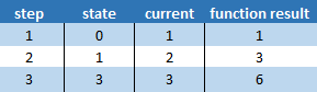
List.Accumulate( {1, 2, 3}, 0, (state, current) => state + current)

Looking at each of those parameters we understand that

{1, 2, 3} is the list upon which calculations will occur
0 is the seed, or starting value.
(state, current) => state + current is the function that defines how values in the list are transformed

The Accumulator Function

The function (state, current) => state + current takes a little understanding.

state is the value of the function at each step/loop.

current is the current item in the list (the first parameter).

Remember that List.Accumulate loops, or iterates, through each value in the list applying the transformation specified by the accumulator function.

In this example when List.Accumulate first runs, state will be 0 which is the initial (seed) value , and current will take the value 1 which is the first value in the list.

The accumulator function adds together state and current, with the result becoming the value state takes for the next loop.

Function Syntax

(state, current) => state + current

Step 1

(0, 1) => 0 + 1

Step 2

(1, 2) => 1 + 2

Step 3

(3, 3) => 3 + 3

Looking at a table showing how state and current change for each step may help understand what is happening.

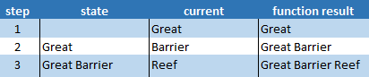
List.Accumulate Example — Concatenating Text

This is very similar to adding numbers, we just change the accumulator function to join the strings in the list, with a space in between each word.

List.Accumulate( {"Great", "Barrier", "Reef"}, "", (state, current) => state & " " & current)

Starting with an empty string, a word from the list (parameter 1) is added to state on each step.

Listing Words Found in Text

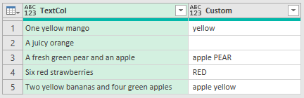
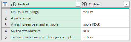
Using the same data as the previous post Searching for Text Strings in Power Query, we have a column of text like so

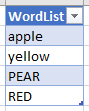
and we want to check each row in the column to see if it contains any of the words in WordList

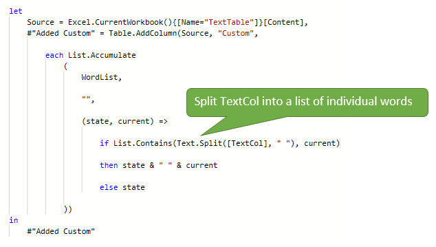
List Found Substrings — Case Sensitive

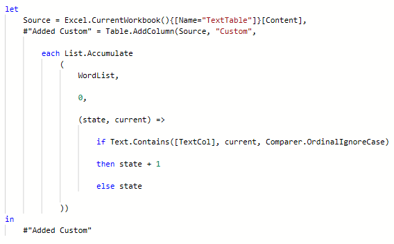
To search for substrings, use Text.Contains. The entire query looks like this

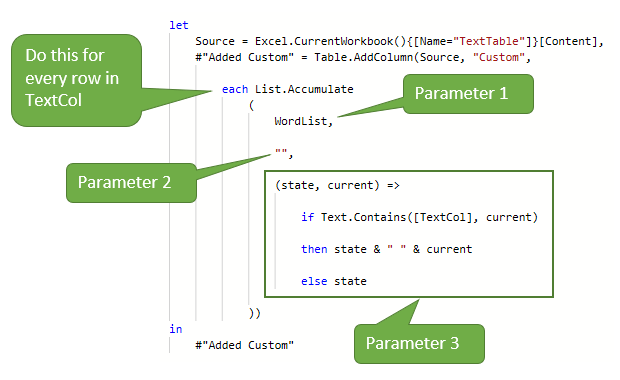
Looking at the parameters, parameter 1 (the list) is WordList, parameter 2 (the seed/initial state) is an empty string «» and parameter 3 (the accumulator function) carries out the following steps.

if the current word in WordList appears in [TextCol]
then state becomes state & » » & current (concatenate the strings)
else state remains unchanged

The accumulator function is called for every word in WordList so the end result will be a string of the words found in TextCol.

This process is carried out for every row of TextCol — that’s what the each keyword signifies.

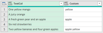
The result is another column listing the words that were found.

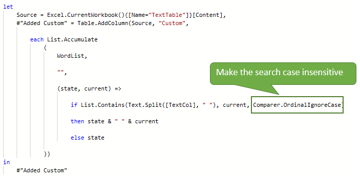
List Found Substrings — Case Insensitive

To make the search for substrings ignore case, add Comparer.OrdinalIgnoreCase as the 3rd parameter to Text.Contains.

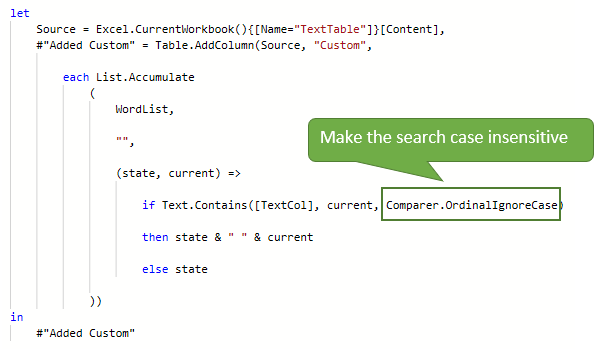
As the search is ignoring case, the words PEAR and RED are now listed.

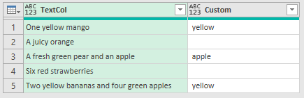
List Exact Matches — Case Sensitive

To do exact matching, that is, apple matches apple, but does not match apples, I’ll use List.Contains, here’s the query.

The only thing that has changed is the if part of the accumulator function which is using List.Contains. As List.Contains requires lists to work with, I need to use Text.Split to split the string in TextCol into a list of individual words.

As this is an exact match search, apple is not listed as a match in row 5.

List Exact Matches — Case Insensitive

To make this search ignore case, use the Comparer.OrdinalIgnoreCase.

Making the search ignore case, the words PEAR and RED are listed again.

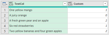
Further Useful Modifications — Counting Matches

As you can see once you get your head around what the accumulator function can do, it’s easy to modify it to do other things, like count the matching words.

To create a query that looks for substrings and ignores case, you can use this code.

Because the function is counting, the seed value needs to be a number, so it’s 0.

To do the actual counting the function just adds 1 to state each time a word is found.

Have fun playing with List.Accumulate and writing your own accumulator functions.

Источник

In this article, we will learn How to Extract all the words except the first in Excel.

Scenario :

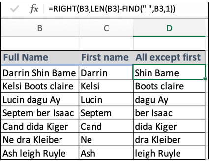
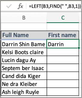
Working with text data in excel. Sometimes we come across the problem of splitting words from the full text. For example splitting full names into first name and last name. Or extracting the names from the given email ids. For situations like these we use LEFT and RIGHT functions in excel along with some basic sense of how excel functions work. How to recognize where to separate the full name like Nedra Kleiber. Here a space character in between the first name and last name. So we direct excel to find the position of first space char in the full name and separate it into two using functions

First name and rest name formula in Excel

Here given a name value as text in the formula. First of all the find function gives the position of first space character and LEN function gives the length of full text. Now the RIGHT function has everything to extract the word.

Remaining name formula syntax:

=RIGHT (text, LEN (text) — FIND (» «, text, 1 ) )

text : full name

» » : Space character given in quotes. Or use char function

1 : nth occurrence of space char. (here 1 is used to specify first occurrence)

First name formula syntax:

text : full name

» » : Space character given in quotes. Or use char function

1 : nth occurrence of space char. (here 1 is used to specify first occurrence)

Example :

All of these might be confusing to understand. Let’s understand how to use the function using an example. Here we are given some sample names and we need to extract the first name and rest of the name in another column. So first we start with a basic formula that is first name extraction. You can provide text values using text in quotes or by using cell reference which is explained here.

First name formula:

Copy and paste the formula in other cells either using CTRL + D or just by stretching the right bottom box of the C3 cell.

As you can see in the above snapshot all the first names are here. Now either you can substitute the first name from the full name with blank to get the last name or use the last name formula explained below.

To get the Last name directly from the full name using the RIGHT function formula is shown below.

Remaining or last name formula:

Copy and paste the formula to different required cells using Ctrl + D or dragging down the right bottom corner of the D3 cell.

As you can see the first name and last name both in different columns separated using the simple excel formulas. Learn more about excel formulas here.

Here are all the observational notes using the formula in Excel
Notes :

Text values in formula be used with between quotes or using cell reference. Using cell reference in excel is the best common practice.
Use the =CHAR(32) function to get the space character in the formula.

Hope this article about How to Extract all the words except the first in Excel is explanatory. Find more articles on calculating values and related Excel formulas here. If you liked our blogs, share it with your friends on Facebook. And also you can follow us on Twitter and Facebook. We would love to hear from you, do let us know how we can improve, complement or innovate our work and make it better for you. Write to us at info@exceltip.com.

Related Articles :

Data Validation in Excel : Data Validation is a tool used to restrict users to input value manually in cell or worksheet in Excel. It has a list of options to choose from.

Way to use Vlookup function in Data Validation : Restrict users to allow values from the lookup table using Data validation formula box in Excel. Formula box in data validation allows you to choose the type of restriction required.

Restrict Dates using Data Validation : Restrict user to allow dates from a given range in cell which lays within Excel date format in Excel.

How to give the error messages in Data Validation : Restrict users to customize input information in the worksheet and guide the input information through error messages under data validation in Excel.

Create Drop Down Lists in Excel using Data Validation : Restrict users to allow values from the drop down list using Data validation List option in Excel. List box in data validation allows you to choose the type of restriction required.

Popular Articles :

50 Excel Shortcuts to Increase Your Productivity : Get faster at your tasks in Excel. These shortcuts will help you increase your work efficiency in Excel.

How to use the VLOOKUP Function in Excel : This is one of the most used and popular functions of excel that is used to lookup value from different ranges and sheets.

How to use the IF Function in Excel : The IF statement in Excel checks the condition and returns a specific value if the condition is TRUE or returns another specific value if FALSE.

How to use the SUMIF Function in Excel : This is another dashboard essential function. This helps you sum up values on specific conditions.

How to use the COUNTIF Function in Excel : Count values with conditions using this amazing function. You don’t need to filter your data to count specific values. Countif function is essential to prepare your dashboard.

Источник

Last year, I wrote a post about using Excel to keep a word bank. It was one of the most popular posts of 2014 and the template was downloaded over 2000 times.

Why use a word bank?

Download

Click on Word Bank 2.13 to download the template.

Delete the example words and start adding your own vocabulary.

Word Bank 2.1 – New Features

The Words sheet was previously known as the Data sheet in the first version of Word Bank.

Go to the Lists sheet and you will notice that Excel will now separate those words into different color coded lists for you.

The Search sheet was previously known as the Word Card sheet in the first version of Word Bank. I had to redesign the Search sheet slightly so that it would be able to search for vocabulary from the different lists.

The Statistics sheet has been updated to not only show the types of words you are learning, but it also displays the percentage of words you have learned. This was intended as a motivational device.

Finally a huge thanks to all the people who read the original word bank post and downloaded version 1.0. I would love to hear from you and get your feedback.

As always, if you have any questions, please leave a comment.

Alternatively you can send me a message on my Facebook page or on Twitter.

Thanks for reading and take care!

Table of contents

#1 – Create a Drop-Down List in Excel

#2 – Create a List of Values from Cells

#3 – Create List through Named Manager

Things to Remember

Recommended Articles

About This Article

Is this article up to date?

Automatically define a list of words in Excel?

Re: Automatically define a list of words in Excel?

Re: Automatically define a list of words in Excel?

Re: Automatically define a list of words in Excel?

Re: Automatically define a list of words in Excel?

Download the Excel Workbook With All the Source Data and Queries in This Post

List.Accumulate

List.Accumulate Example — Adding Numbers

The Accumulator Function

Function Syntax

Step 1

Step 2

Step 3

List.Accumulate Example — Concatenating Text

Listing Words Found in Text

List Found Substrings — Case Sensitive

List Found Substrings — Case Insensitive

List Exact Matches — Case Sensitive

List Exact Matches — Case Insensitive

Further Useful Modifications — Counting Matches