Listing rows in excel - Word и Excel - помощь в работе с программами

Download Article

If you’re wondering how to create a multiple-line list in a single cell in Microsoft Excel, you’ve come to the right place. Whether you want a cell to contain a bulleted list with line breaks, a numbered list, or a drop-down list, inserting a list is easy once you know where to look. This wikiHow will teach you three helpful ways to insert any type of list to one cell in Excel.

1

Double-click the cell you want to edit. If you want to create a bullet or numerical list in a single cell with each item on its own line, start by double-clicking the cell into which you want to type the list.
2
Insert a bullet point (optional). If you want to preface each list item with a bullet rather than a number or other character, you can use a key shortcut to insert the bullet symbol. Here’s how:
- Mac: Press Option + 8.
- Windows:
  - If you have a numeric keypad on the side of your keyboard, hold down the Alt key while pressing 7 on the keypad.^[1]
  - If not, click the Insert menu, select Symbol, type 2022 into the «Character code» box at the bottom, and then click Insert.
  - If 2022 didn’t bring up a bullet point, select the Wingdings font instead, and then enter 159 as the character code. You can then click Insert to add the bullet point.
Advertisement
3
Type your first list item. Don’t press Enter or Return after typing.
- If you want your list to be numbered, preface the first list item with 1. or 1).
4

Press Alt+↵ Enter (PC) or Control+⌥ Option+⏎ Return on a Mac. This adds a line break so you can start typing on the next line of the same cell.^[2]
5

Type the remaining list items. To continue your list, just enter another bullet point on the second line, type the list item, and press Alt + Enter or Control + Option + Return to open a new line. When you’re finished, you can click anywhere else on your sheet to exit the cell.

1
Create your list in another app. If you’re trying to paste a bullet list (or other type of list) into a single cell rather than have it spread across multiple cells, there’s a trick to pasting the list. Start by creating your list in an app like Word, TextEdit, or Notepad.
- If you create a bulleted list in Word, the bullets will copy over to your cell when pasted into Excel. Bullets may not copy from other apps.
2

Copy the list. To do this, just highlight the list, right-click the highlighted area, and then select Copy.
3

Double-click a cell in Excel. Double-clicking the cell before pasting makes it so the list items will all appear in the same cell.
4

Right-click the cell. The context menu will expand.
5

Click the clipboard icon under «Paste Options.» The icon has a clipboard and a black rectangle. This pastes the list into the cell you double-clicked. Each list item will appear on its own line within the same cell.

1

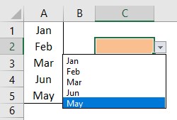
Open the workbook in which you want to create a drop-down list. If you want to be able to click a cell to view and select from a drop-down list, you can create a list with Excel’s data validation tool.^[3]
2
Create a new worksheet in the workbook. You can do this by clicking the + next to the existing workbook sheets at the bottom of Excel. This worksheet is where you’ll enter the items that you want to appear in your drop-down list.
- After you create the list on a separate sheet and add it to a table, you’ll be able to create a drop-down list containing the list data in any cell you want.
3
Type each list item into a single column. Enter every possible list choice into its own separate cell. The items you type will all be available in the drop-down list.
- If you plan to make a lot of drop-down menus and want to use this same sheet to create all of them, add a header to the top of the list. For example, if you’re making a list of cities, you could type City into the first cell. This header won’t actually appear on the drop-down list you create—it’s just for organization on this sheet that contains list data.
4

Highlight the entire table and press Ctrl+T. Include the header at the top of the list when highlighting. This opens the Create Table dialog.
5
Choose a header option and click OK. If you added a header to the top of your list, check the box next to «My table has headers.» If not, make sure there is no checkmark there before clicking OK.
- Now that your list is in a table, you can make changes to it after creating your drop-down list, and your drop-down list will update automatically.
6

Sort the list alphabetically. This will keep your list organized once you add it to your sheet. To do this, just click the arrow next to your header cell and select Sort A to Z.
7

Click the cell on the worksheet in which you want to add the list. This can be any cell on any worksheet in the workbook.
8

Type a name for the list into the cell. This is the cell where the list will appear, so give it a name that indicates the type of option you should choose from that list. For example, if you made a list of cities, you could type City here.
9

Click the Data tab and select Data Validation. Make sure the cell is selected before doing this. If you don’t see Data Validation in the toolbar, click the icon in the «Data Tools» section that has two black rectangles with a green checkmark and a red circle with a line through it. This opens the Data Validation window.
10

Click the «Allow» menu and select List. Additional options will expand.
11

Click the up-arrow in the «Source» field. This minimizes the Data Validation window so you can select your list data.
12

Select the list (without the header) and press ↵ Enter or ⏎ Return. Click back over to the tab that has your list data and drag the mouse cursor over just the list items. Pressing Enter or Return will add the range to the «Source» field.
13

Click OK. The selected cell now has a drop-down list. If you need to add or remove items from the list, you can simply make those changes on your new worksheet and they’ll automatically propagate to the list.

Ask a Question

200 characters left

Include your email address to get a message when this question is answered.

Submit

Thanks for submitting a tip for review!

About This Article

Article SummaryX

1. Double-click the cell.
2. Press Alt + 7 or Option + 8 to add a bullet point.
3. Type a list item.
4. Press Alt + Enter (PC) or Control + Option + Return (Mac) to go to the next line.
5. Repeat until your list is finished.

Did this summary help you?

Thanks to all authors for creating a page that has been read 62,222 times.

Is this article up to date?

Источник

When we need to collect data from others, they may write different things from their perspective. Still, we need to make all the related stories under one. Also, it is common that while entering the data, they make mistakes because of typo errors. For example, assume in certain cells, if we ask users to enter either “YES” or “NO,” one will enter “Y,” someone will insert “YES” like this, and we may end up getting a different kind of results. So in such cases, creating a list of values as pre-determined values allows the users only to choose from the list instead of users entering their values. Therefore, in this article, we will show you how to create a list of values in Excel.

Create List in Excel
- #1 – Create a Drop-Down List in Excel
- #2 – Create List of Values from Cells
- #3 – Create List through Named Manager
- Things to Remember
- Recommended Articles

You can download this Create List Excel Template here – Create List Excel Template

#1 – Create a Drop-Down List in Excel

We can create a drop-down list in Excel using the “Data Validation in excelThe data validation in excel helps control the kind of input entered by a user in the worksheet.read more” tool, so as the word itself says, data will be validated even before the user decides to enter. So, all the values that need to be entered are pre-validated by creating a drop-down list in Excel. For example, assume we need to allow the user to choose only “Agree” and “Not Agree,” so we will create a list of values in the drop-down list.

In the Excel worksheet under the “Data” tab, we have an option called “Data Validation” from this again, choose “Data Validation.”

As a result, this will open the “Data Validation” tool window.

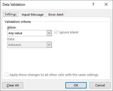
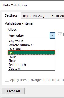
The “Settings” tab will be shown by default, and now we need to create validation criteria. Since we are creating a list of values, choose “List” as the option from the “Allow” drop-down list.

For this “List,” we can give a list of values to be validated in the following way, i.e., by directly entering the values in the “Source” list.

Enter the first value as “Agree.”

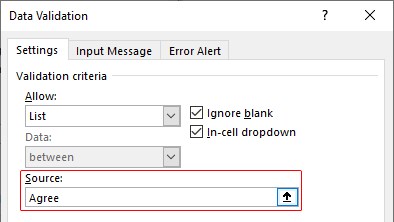
Once the first value to be validated is entered, we need to enter “comma” (,) as the list separator before entering the next value. So, enter “comma” and enter the following values as “Not Agree.”

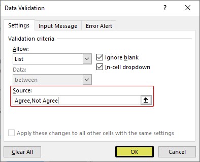
After that, click on “Ok,” and the list of values may appear in the form of the “drop-down” list.

#2 – Create a List of Values from Cells

The above method is to get started, but imagine the scenario of creating a long list of values or your list of values changing now and then. Then, it may get difficult to return and edit the list of values manually. So, by entering values in the cell, we can easily create a list of values in Excel.

Follow the steps to create a list from cell values.

We must first insert all the values in the cells.
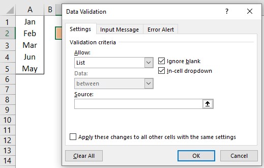
Then, open “Data Validation” and choose the validation type as “List.”
Next, in the “Source” box, we need to place the cursor and select the list of values from the range of cells A1 to A5.
Click on “OK,” and we will have the list ready in cell C2.

So values to this list are supplied from the range of cells A1 to A5. Any changes in these referenced cells will also impact the drop-down list.

For example, in cell A4, we have a value as “Apr,” but now we will change that to “Jun” and see what happens in the drop-down list.

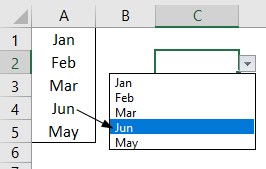
Now, look at the result of the drop-down list. Instead of “Apr,” we see “Jun” because we had given the list source as cell range, not manual entries.

#3 – Create List through Named Manager

There is another way to create a list of values, i.e., through named ranges in excelName range in Excel is a name given to a range for the future reference. To name a range, first select the range of data and then insert a table to the range, then put a name to the range from the name box on the left-hand side of the window.read more.

We have values from A1 to A5 in the above example, naming this range “Months.”

Now, select the cell where we need to create a list and open the drop-down list.

Now place the cursor in the “Source” box and press the F3 key to an open list of named ranges.

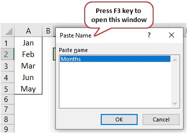
As we can see above, we have a list of names, choose the name “Months” and click on “OK” to get the name to the “Source” box.

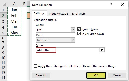
Click on “OK,” and the drop-down list is ready.

Things to Remember

The shortcut key to open data validation is “ALT + A + V + V.“
We must always create a list of values in the cells so that it may impact the drop-down list if any change happens in the referenced cells.

Introduction to Rows and Column in Excel

In Microsoft excel, if we open a new workbook, we can see that sheet will contain tables with light grey color. Basically excel is a tabular format which contains n number of rows and columns, where rows in excel will be in a horizontal line, and column in excel will be in a vertical line.

In excel, we can find each row by its row number, which is shown in the below screenshot, which shows vertical numbers on the left side of each sheet.

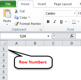
As we can see in the above screenshot that each row can be identified by their row numbers like 1, 2, 3 etc.
Whereas we can find the column in excel, which can be identified by the column header like A, B, C. which will be shown normally in all excel sheets, which are shown below.

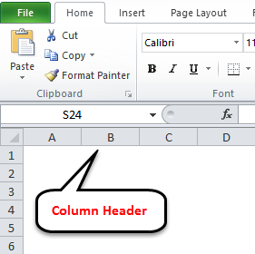
In Excel, each column is named by its header, which shows the column header horizontally at the top of the excel sheet.

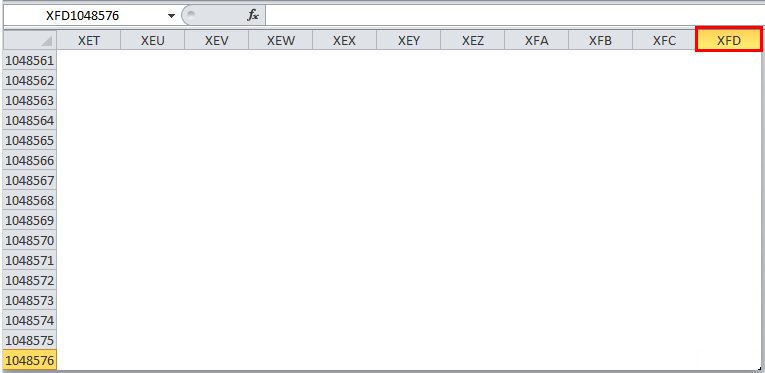
In Microsoft Excel 2010 and the latest version, we have row numbers ranging from 1 to 1048576 in 1048576, whereas the column ranges from A to XFD in a total of 16384 columns which is shown in the below screenshot.

Rows in excel range from 1 to 1048576, which is highlighted in red mark

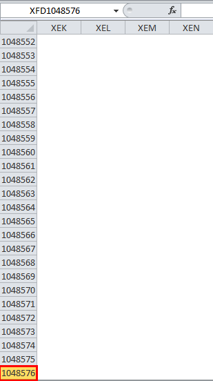
The column in excel ranges from A to XFD, which is highlighted in red mark.

Rows and Column Navigation in excel

In this example, we will see how to navigate rows and columns with the below examples.

We can find the last row of excel by using the keyboard shortcut key CTRL+DOWN NAVIGATION ARROW KEY, or else we can use the vertical scrollbars to go to the end of the row.

We can find the last column of excel by using the CTRL+RIGHT NAVIGATION ARROW KEY, or else we can use the horizontal scrollbars to go to the end of the column.

How to Select Rows and Column in excel?

In this example, we will learn how to select the rows and columns in excel.

You can download this Rows and Column Excel Template here – Rows and Column Excel Template

Rows and Column in Excel – Example#1

Normally, when we open a workbook, we can see that sheet contains tabular rows and columns where each row is specified by their row number and column specified by their column header.

Consider the below example, which has some data in an excel sheet. Here we will see how to select the rows and columns.

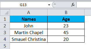
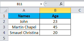
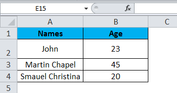
In the above screenshot, we can see that names and age column have their own header name A and B, and each row has its own row number.

In excel, each time when we select a row or column, “Name Box” will display the specific row number and column name, which is shown in the below screenshot.

In this example, we will select the Names and Age, and let’s see how the rows and column header is getting displayed.

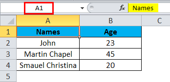
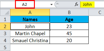
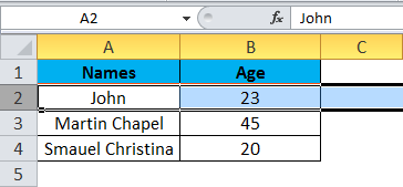
Step 1 – First, select the cell Name John.

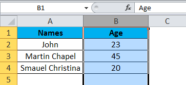
Step 2 – Once you select the cell name, John, we will get the row number and column name as A2 in the name box, which means that we have selected A column second row as A2, shown below screenshot with yellow highlighted.

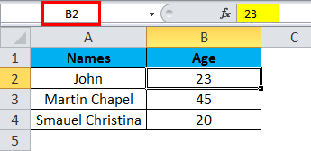
Step 3 – Now select cell 23, where it will show the selected cell is B2 which is shown in the below screenshot with yellow highlighted.

Step 4 – Now select all the names and columns to show that we have 4 rows and 2 columns shown in the below screenshot.

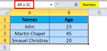
In this way, we can identify the row number and column name by selecting each cell in excel.

Example#2 – Changing Row and Column Size

This example shows how to change the row and column size by using the following examples.

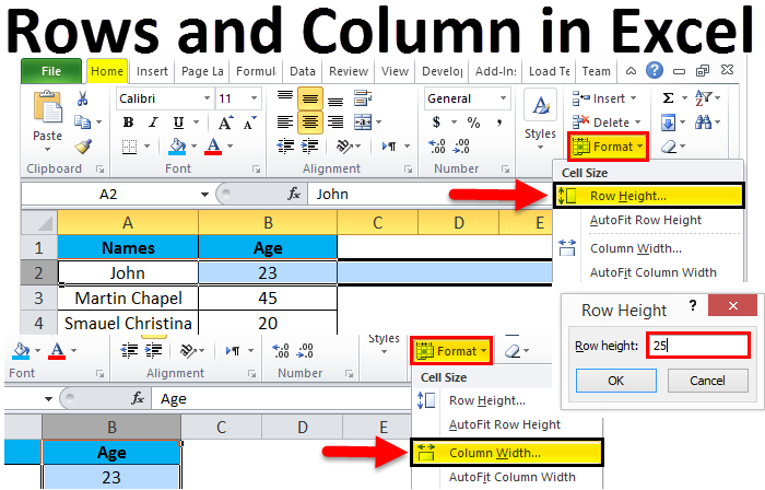
Excel row and column width size can be modified by using the format option in the HOME menu, which is shown below.

Using the format menu, we can change the row and column width where we have the list option, which are as follows:

ROW HEIGHT– This is used to adjust the row height.
AUTOFIT ROW HEIGHT– This will automatically adjust the row height.
COLUMN WIDTH – This is used to adjust column width.
AUTOFIT COLUMN WIDTH– This will automatically adjust the column width.

Let’s consider the below example to change the row and column width. Follow the below steps.

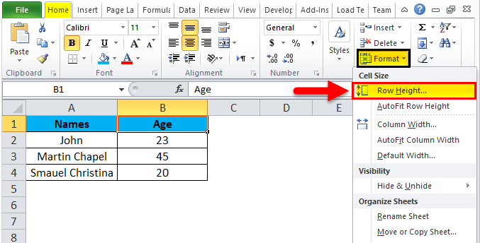
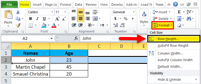
Step 1 – First, select the second row as shown in the below screenshot.

Step 2 – Go to the Format menu and click on ROW HEIGHT, as shown below.

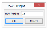
Step 3 – Once we select the ROW HEIGHT, we will get the below dialog box to change the height of the row.

Step 4 – Now increase the row height to 25 so that the selected row height will get increased, as shown in the below screenshot.

We can see that row height has been increased when compared to the previous one; alternatively, we can change the row height by using the mouse.

Step 5 – Now go to the second option in the format list called AUTOFIT ROW HEIGHT, which will automatically reset the row to its original height.

Step 6 – Select the same row and go to the Format menu.

Step 7 – Now select the “AutoFit Row Height” as shown below.

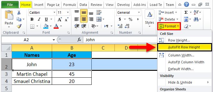
Once we click on the “AutoFit Row Height” option, the row height will reset to the original position, shown below.

Adjusting Column Width

We can adjust the column width in the same way by using the format option.

Step 1 – First, click on the cell B cell as shown below.

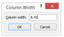
Step 2 – Now go to the Format menu and click on column width as shown in the below screenshot.

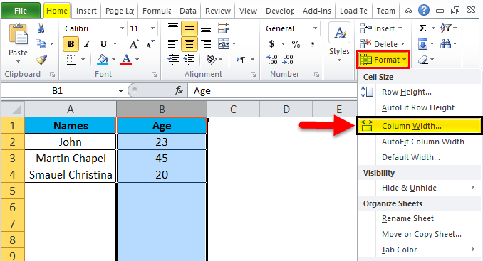
Once we click on the Column width, we will get the below dialog box to increase the column width, as shown below.

Step 3 – Now increase the column width by 15 to increase the selected column width.

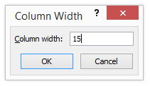
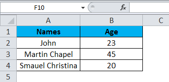
In the above screenshot, we can see that column width has been increased; alternatively, we can adjust the column width by using the mouse where if we place the mouse cursor, we will get the + plus mark sign near to the column.

Step 4 – Now click on the next option called “AutoFit Column width”. So that the selected column will get reset to its original size, which is shown below.

Things to Remember

In excel, we can delete and insert multiple rows and columns.
We can hide the specific row and columns using the hide option.
Row and column cells can be protected by locking the specific cells.

Example

You’ll most probably need to number rows in Excel for serial numbering in your dataset so here’s an example of where it can be applied:

We have an employee database of a school which can do with some sequential numbering. Our aim is to serially number this dataset in column B.

With some methods, you will get static numbering of rows and dynamic numbering with the rest. If that is important to you, we’ve mentioned which method delivers which results with the subheadings.

Let’s get numbering!

Using Fill Handle

Static numbering

Let’s use the simplest method first which requires no functions or fancy features. We use the Fill Handle. The Fill Handle is the tiny square that appears at the bottom-right corner of the selected cell(s). The Fill Handle recognizes the formula or pattern contained in the selected cell(s) and copies them down to the extended range. With this feature, we can number the rows in our dataset. See below how it’s done:

In the column where you want the serial numbers, enter 1 and 2 in the first and second rows:

This will help the Fill Handle pick up on the pattern.
Select these two cells containing the numbers 1 and 2. The Fill Handle will appear in the bottom corner.

Hover the cursor on the Fill Handle until the cursor changes to a cross.

Now click and drag the Fill Handle to where you want the numbered rows. We want the rows numbered to 10 so we’ll drag the handle down to B12. The callout bubble will display the value for the target cell as you click and drag.

If you want to number the entire dataset’s rows, double-click the Fill Handle and it will number all the rows of the dataset that have the adjacent column filled.

When you release the left mouse button, the cells will be auto-filled with the numbered rows using the Fill Handle:

Using Fill Series Option

Static numbering

Here’s another feature that acts as a filler. To fill the rows with serial numbers, you can give Fill Series a go. Given its few options, you’ll find it quite handy for filling in numbers and dates in the specified steps. For now, we only need sequential numbering so we’ll head onto the steps right away:

Enter the number 1 in the first row of the column you want numbered.
Select the cell so that Fill Series can create the series to fill the column based on this number.
Select the Fill icon in the Editing section of the Home tab and then select the Series option from the menu.

The Series dialog box will be launched.
In the dialog box make the following selections:
- Select the Columns radio button in the Series in section
- Select the Linear radio button in the Type
- Enter the Step value and Stop value for your number series.
For us, that would be 1 and 10.
The Step value is the number by which you want the numbers to increase. E.g. if we enter 2 here, the numbers in the series would go 1, 3, 5….. Since we want regular numbering, we have entered 1 as the Step value.
Stop value is the number where you want the series to end.

Click on the OK button when done.

With these steps, the column will be filled with the given number series:

Incrementing Previous Row Number by 1

Static numbering

Now we move on to the formulas for numbering rows in Excel and it only makes sense to start with the simplest one first. By adding 1 to the previous row number, we can create a sequence of numbers. Here’s what you need to do if you choose this method:

Start by entering «1» in the first cell where the serial numbers will be.
In the next cell of the column, add 1 to the previous cell using this formula:

=B3+1

In this formula, B3 will be the cell containing the number 1. Adding 1 to B3 will result in the number 2. And this is how it will keep going. The next cell will be B4+1 which will result in 3, so on and so forth. In this way, the numbers will keep increasing serially.

Now extend the formula to where you want the last number.
With this plain arithmetic formula, the rows will be numbered up to 10:

Using ROW Function

Dynamic numbering

And now we will number rows using a simple function, the ROW function. The ROW function returns the row number of a referred cell. So, no matter where we are on the active worksheet, if you refer a certain cell, the ROW function would return the specified cell’s row number. With the steps below, we’ll show you how we make the ROW function work for returning numbered rows:

=ROW()-2

The ROW function has been used on its own to return the number of the row the formula is entered in and then we deduct that figure by 2. Why? Our target cell is B3 so =ROW() would return 3. To make the ROW function return 1 as the first number, we have deducted 2 in the formula. You will need to adjust this value according to the row your target cell is in.

As the formula is copied down, it will return the row number and then 2 will be subtracted. E.g. in the next instance, the row number is 4. 4-2 = 2. The next row number will be 5. 5-2 = 3 and so on.

We have chosen this formula since our numbering was starting from B3. If you’re already starting from row 1, you can enter the formula as:

=ROW()

This formula will return the row number of the cell the formula is entered in.

Note: Both the ROW formulas suggested above will bring about dynamic results that recalculate with additions and deletions.

Using COUNTA Function

Dynamic numbering

Going good up until now. Rows are being numbered, the morning birds are taking their cue and the sun is rising somewhere. And then you realize that as opposed to a continuous dataset, your data has some blank rows that don’t need numbering. Challenge accepted; we have the COUNTA function at our disposal.

The COUNTA function counts the number of cells in a range that are not empty. COUNTA will count the non-empty cells in the adjacent column and, with the IF and ISBLANK functions, will return nothing if the adjacent cell is blank. Sounds like a plan. Let’s see all the works. we begin with this formula:

=IF(ISBLANK(C3),"",COUNTA($C$3:C3))

As per the IF function, C3 will be checked by the ISBLANK function as to whether it’s a blank cell or not. If this tests true, the IF function will return an empty text string «».

If the cell is not blank, then the COUNTA function will start counting the non-blank cells from $C$3 (mentioning the number as an absolute reference locks the cell in the formula so that as the formula is copied down, the reference remains the same) and return the count as the answer of the formula.

In the first instance, the count from C3 only makes 1 cell so 1 is the result.

In the next instance, COUNT counts C3 and C4 and therefore returns 2. In the third instance, the adjacent cell i.e. C5 is blank so this row has not been numbered.

Note: The results of using this formula are dynamic; with any change of addition or deletion of data, the numbering will recalculate and adjust accordingly.

Using OFFSET Function

Dynamic numbering

Rows in Excel can also be numbered using the OFFSET function. It’s a slightly “off” the norm method but a method nonetheless and it requires you to start the column without a header; you’ll see why in a while.

The OFFSET function returns the value of the cell which is the given numbers of rows and columns from the specified cell. We will use this concept to then add 1 to each result to create serial numbering. Below is the demonstration with the formula:

=OFFSET(B3,-1,0)+1

Now you’ll see why a blank column header was a prerequisite. Let’s understand the path in the formula. The cell specified is B3 itself. From there, OFFSET trails to -1 rows. This means B2. now in the third parameter of the formula, from B2 we need to shift to 0 columns which still leads to B2.

This means that using the OFFSET function, we will be referring to the previous cell in the same column. In the last bit of the formula, we have +1 which adds the number 1 to the value of B2. Since B2 is blank, 0+1 = 1. 1 is the outcome here. This is why we needed the header to be blank.

In the next instance, OFFSET will lead to B3 and add 1 to B3’s value. 1+1 = 2. That is how the rest of the rows will be numbered in succession.

Once you are done, you can copy and paste the values over themselves and add the column header if you so wish. The values are pasted back so that they are not formula-reliant and won’t cause errors.

Note: As long as the column header is absent, the results of this formula are dynamic. If you wish to add the column header, you will have to paste back the values or you can choose another method if want to retain the column header and the dynamic numbering.

Using SUBTOTAL Function

Dynamic numbering

And again, things were looking bright until you were hit with another requirement. You need to filter data but that would also filter the serial numbers. Now that’s a problem but not a problem we can’t work around. Enter SUBTOTAL function.

The SUBTOTAL function returns a subtotal in a dataset. While we will be using the COUNTA function via SUBTOTAL, SUBTOTAL will help to dynamically recalculate the row numbers as the data is filtered. Want to see how that works? We’ve got the formula to number rows with the SUBTOTAL function right ahead:

=SUBTOTAL(3,$C$3:C3)

The SUBTOTAL function presents a list of functions to choose from in the Formula AutoComplete. This parameter will determine what kind of subtotal you want to enter.

After selecting the function, the next input is the cell reference. As shown in the COUNTA function section above, we will enter $C$3:C3 as the range so that the count always begins from $C$3. As the formula is filled downward, the count will continue up until the target cell.

Now try filtering your data.

The row numbers will be recalculated with the filtered data serially numbered:

With the new serial number selected, we can note in the formula that the count for non-blank cells has started from $C$3 to C4 instead of C3. In this way, the count will begin from $C$3 and jump directly to the first filtered cell in the C column.

Creating Calculated Column in Excel Table

Dynamic numbering

Last but not least, let’s table it! An Excel table talks the talk and walks the walk and there are many convenient features it offers. The one helping us today is a calculated column; enter one formula and you’ll have numbered rows. Excel tables are known for being dynamic in their very nature and a calculated column also provides that ease. Nothing short of Excel magic. The complete tricks (read steps) to do this are as follows:

Select any cell in the dataset. This will help Excel identify the range to create the Excel table.
In the Home tab, go to the Styles section and click on the Format as a Table Select the table style from the menu or create your own.

Now a small dialog box will appear confirming the identified range of the intended Excel table. Correct the range if required.
If your table has headers, leave the My table has headers checkbox checked.
Then click on the OK button to close the dialog box and apply the table.

An Excel table will be created on the provided range:

Now, enter this formula in any cell in the column where you want the numbers:

=ROW()-ROW(Table1[#Headers])

As a calculated column, when the formula is entered, all the rows will automatically be serially numbered:

And that’s your job done!

And that’s our tutorial done! The solutions may be numbered but so are the problems and today you saw how to tackle numbering rows in Excel in many different ways.

Filtering data and dealing with gaps in the data are two hitches you might face when numbering rows but today you’ve learned how to breeze through them. We’re up for making other hitches easy, breezy and we’re on it too so we’ll see you around another Excel trick!

Источник

Introduction

In Power Automate, during certain scenarios, we must traverse all the records in the excel file table and based on a few conditions content in excel to be updated. List Rows action present under Excel Online(Business) Connector in power automate can be used. As an example scenario of updating eligibility of Employees based on Age explained here.

Step 1

Login to the required Power Apps environment using URL make.powerapps.com by providing username and password and click on Flows on the left-hand side as shown in the below figure.

Step 2:

After Step 1, Click on New Flow and select instant cloud flow and provide the trigger as Manually trigger a flow and click on Create as shown in the below figure.

Step 3:

After Step 2, name the flow as Working With List Rows Present in Excel Table OneDrive and take List rows present in a table action under Excel Online(Business) as shown in the below figure.

Step 4:

After Step 3, name step as List rows present in a table [ Employee Table] provide the input values

Location : OneDrive for Business

Document Library: OneDrive

File : ExcelWorkBooks/Employee.xlsx

Table : Table1

as shown in the below figure.

Step 5:

After Step 4, take action Apply to each and then under Select an output from previous steps select value from List rows present in a table [ Employee Table]

as shown in the below figure.

Step 6:

After Step 5, inside Apply to each Step, add an action as condition and inside condition provide the following values

First Value : float(items('Apply_to_each')?['Age'])

Condition : is greater than or equal to

Value to compare : 18

as shown in the below figure.

Step 7:

After Step 6, under if yes block, select action update a row under Excel Online(Business) and provide below values

Location : OneDrive for Business

Document Library: OneDrive

File : ExcelWorkBooks/Employee.xlsx

Table : Table1

Key Column : Sno

Key Value : Sno – selected from [items('Apply_to_each')?[ Sno]]

Date - @{triggerOutputs()['headers']['x-ms-user-timestamp']}

Comments: Eligible for Vaccination

as shown in the below figure.

Step 8:

After Step 7, make sure in Employees Excel File under table1, columns are

as shown in the below figure.

Step 9:

After Step 8, now save and manually test the flow post providing the connections for Dataverse and observe that values in spreadsheet gets populated as shown in the below figure.

And observe excel file gets filled with values only for the Employees whose age was greater than equal to 18 years as shown in the below figure

Note:

Make sure to save and run the flow whenever you try expressions.
Make sure to under Step 6 condition as the value in excel table is an object cannot be compared with an integer value, so that’s why float function was used on Age object which will convert from string to float value then only flow can easily compare between numbers otherwise we get an exception.
Make sure to use proper columns in spreadsheet are used in flow

Conclusion

In this way, one can iterate through list of records present in excel table OneDrive and based on condition updates rows and for bulk files this is an efficient way so as to reduce huge manual work.

Источник

To keep you valued readers engaged and updated with the latest offerings of Microsoft and the IT solutions that my organization provides, the marketing team here works with great zeal to identify readership interests and preference on the regularly published blogs.

One evident task in this effort is to keep a track of number of views, comments for each published blog. This may not at start look like an arduous task, but considering the volume over a period, the number does look daunting.

Fetching some update like this might not qualify for some sophisticated coding effort, hence, I tried to create a Power Automate solution for my team, and only they could confirm if that helped. However, my entire journey in this attempt has been quite refreshing with discovery of new actions to Power Automate.

Introduction

The text above was an ode to my team. My actual blog work starts here.

Unlike my other Flows, this one is short and crisp.

For sake of simplicity, and to stay uptight, I am enumerating only the main actions of the entire flow.

List rows in an online excel table
Update data in the online excel table against each corresponding row fetched from #1

Between #1 and #2, I have initialized and set values in some variables that I need to use in #2, however that is something quite specific to my need, so I have voluntarily skipped from focusing on that.

Get Set Go

The below screen shot displays my online excel table with 3 columns, namely ‘BlogURL’, ‘Number of Views’ and ‘Number of Comments’.

The trigger of your flow can be anything, in my case it is a recurring activity with a set periodic recurrence, hence I directly jump to the main actions of the flow.

List rows present in a table

I have used an O365 excel file, hence the Location, Document Library and File fields point to my file.

Table is the range of cells identified for any activity.

To help flow choose the Table, I opened the excel file in a desktop app and selected my range of column headers and clicked on Home > Format as Table to identify the table.

This action shows up a new menu option Table Design which allows to name the table.

Note: The identification of Table in excel must be performed prior to creating the Flow.

You may also like : Power Automate Conditional Substring Pattern Filtration of Excel Tabular Data

Update a Row

The UI that comes up on this action, prompts me to enter the file location details (since it may not be the same file where update might be required). After pointing out the file location details and the Table (similar to that done in the previous step), Flow intelligently shows options for Key Column based on the selected table; this is for identification of the unique row where update should be done.

All available columns of the table are listed in this action for any update to be made to them.

The Key Value can be any text that you think uniquely identifies the excel table row. In my case, I am using the BlogURL from the fetched excel table, which shows up in my Dynamic Content.

Flow is quite intelligent to understand that the value in BlogURL are multiple (since it is fetched from the entire excel table), hence automatically this action gets encapsulated inside Apply to each block, to run as a loop for each BlogURL column value fetched from the excel table.

I have initialized and set a few variables that I am using to update my excel row data for the columns I need to update, rest column values can be left blank if no update is to be made.

On the Finish Line

This blog may seem to be quite rushed since I omitted a major chunk of initializing and setting variables values, as I wanted to stay focused to the actual actions.

What may be important, is to outline that while I am updating values in the same table, the Update a Row action is not limited to the excel table from which rows were listed in step #1. The update action can be performed on any other online excel table by pointing to the appropriate online O365 Excel Location and Table details and selecting the desired Key Column and Key Value to update respective column(s) data for row(s) matching the key value.

Finally, as I pen down this blog, I leave my Flow to run to fill in all the missing details of the excel table as in the image below.

Источник

На чтение 18 мин. Просмотров 74.9k.

сэр Артур Конан Дойл

Это большая ошибка — теоретизировать, прежде чем кто-то получит данные

Эта статья охватывает все, что вам нужно знать об использовании ячеек и диапазонов в VBA. Вы можете прочитать его от начала до конца, так как он сложен в логическом порядке. Или использовать оглавление ниже, чтобы перейти к разделу по вашему выбору.

Рассматриваемые темы включают свойство смещения, чтение
значений между ячейками, чтение значений в массивы и форматирование ячеек.

Содержание

Краткое руководство по диапазонам и клеткам
Введение
Важное замечание
Свойство Range
Свойство Cells рабочего листа
Использование Cells и Range вместе
Свойство Offset диапазона
Использование диапазона CurrentRegion
Использование Rows и Columns в качестве Ranges
Использование Range вместо Worksheet
Чтение значений из одной ячейки в другую
Использование метода Range.Resize
Чтение Value в переменные
Как копировать и вставлять ячейки
Чтение диапазона ячеек в массив
Пройти через все клетки в диапазоне
Форматирование ячеек
Основные моменты

Краткое руководство по диапазонам и клеткам

Функция	Принимает	Возвращает	Пример	Вид
Range	адреса ячеек	диапазон ячеек	.Range(«A1:A4»)	$A$1:$A$4
Cells	строка, столбец	одна ячейка	.Cells(1,5)	$E$1
Offset	строка, столбец	диапазон	.Range(«A1:A2») .Offset(1,2)	$C$2:$C$3
Rows	строка (-и)	одна или несколько строк	.Rows(4) .Rows(«2:4»)	$4:$4 $2:$4
Columns	столбец (-цы)	один или несколько столбцов	.Columns(4) .Columns(«B:D»)	$D:$D $B:$D

Введение

Это третья статья, посвященная трем основным элементам VBA. Этими тремя элементами являются Workbooks, Worksheets и Ranges/Cells. Cells, безусловно, самая важная часть Excel. Почти все, что вы делаете в Excel, начинается и заканчивается ячейками.

Вы делаете три основных вещи с помощью ячеек:

Читаете из ячейки.
Пишите в ячейку.
Изменяете формат ячейки.

В Excel есть несколько методов для доступа к ячейкам, таких как Range, Cells и Offset. Можно запутаться, так как эти функции делают похожие операции.

В этой статье я расскажу о каждом из них, объясню, почему они вам нужны, и когда вам следует их использовать.

Давайте начнем с самого простого метода доступа к ячейкам — с помощью свойства Range рабочего листа.

Важное замечание

Я недавно обновил эту статью, сейчас использую Value2.

Вам может быть интересно, в чем разница между Value, Value2 и значением по умолчанию:

' Value2
Range("A1").Value2 = 56

' Value
Range("A1").Value = 56

' По умолчанию используется значение
Range("A1") = 56

Использование Value может усечь число, если ячейка отформатирована, как валюта. Если вы не используете какое-либо свойство, по умолчанию используется Value.

Лучше использовать Value2, поскольку он всегда будет возвращать фактическое значение ячейки.

Свойство Range

Рабочий лист имеет свойство Range, которое можно использовать для доступа к ячейкам в VBA. Свойство Range принимает тот же аргумент, что и большинство функций Excel Worksheet, например: «А1», «А3: С6» и т.д.

В следующем примере показано, как поместить значение в ячейку с помощью свойства Range.

Sub ZapisVYacheiku()

    ' Запишите число в ячейку A1 на листе 1 этой книги
    ThisWorkbook.Worksheets("Лист1").Range("A1").Value2 = 67

    ' Напишите текст в ячейку A2 на листе 1 этой рабочей книги
    ThisWorkbook.Worksheets("Лист1").Range("A2").Value2 = "Иван Петров"

    ' Запишите дату в ячейку A3 на листе 1 этой книги
    ThisWorkbook.Worksheets("Лист1").Range("A3").Value2 = #11/21/2019#

End Sub

Как видно из кода, Range является членом Worksheets, которая, в свою очередь, является членом Workbook. Иерархия такая же, как и в Excel, поэтому должно быть легко понять. Чтобы сделать что-то с Range, вы должны сначала указать рабочую книгу и рабочий лист, которому она принадлежит.

В оставшейся части этой статьи я буду использовать кодовое имя для ссылки на лист.

Следующий код показывает приведенный выше пример с использованием кодового имени рабочего листа, т.е. Лист1 вместо ThisWorkbook.Worksheets («Лист1»).

Sub IspKodImya ()

    ' Запишите число в ячейку A1 на листе 1 этой книги    
     Sheet1.Range("A1").Value2 = 67

    ' Напишите текст в ячейку A2 на листе 1 этой рабочей книги
    Sheet1.Range("A2").Value2 = "Иван Петров"

    ' Запишите дату в ячейку A3 на листе 1 этой книги
    Sheet1.Range("A3").Value2 = #11/21/2019#

End Sub

Вы также можете писать в несколько ячеек, используя свойство
Range

Sub ZapisNeskol()

    ' Запишите число в диапазон ячеек
    Sheet1.Range("A1:A10").Value2 = 67

    ' Написать текст в несколько диапазонов ячеек
    Sheet1.Range("B2:B5,B7:B9").Value2 = "Иван Петров"

End Sub

Свойство Cells рабочего листа

У Объекта листа есть другое свойство, называемое Cells, которое очень похоже на Range . Есть два отличия:

Cells возвращают диапазон только одной ячейки.
Cells принимает строку и столбец в качестве аргументов.

В приведенном ниже примере показано, как записывать значения
в ячейки, используя свойства Range и Cells.

Sub IspCells()

    ' Написать в А1
    Sheet1.Range("A1").Value2 = 10
    Sheet1.Cells(1, 1).Value2  = 10

    ' Написать в А10
    Sheet1.Range("A10").Value2 = 10
    Sheet1.Cells(10, 1).Value2  = 10

    ' Написать в E1
    Sheet1.Range("E1").Value2 = 10
    Sheet1.Cells(1, 5).Value2  = 10

End Sub

Вам должно быть интересно, когда использовать Cells, а когда Range. Использование Range полезно для доступа к одним и тем же ячейкам при каждом запуске макроса.

Например, если вы использовали макрос для вычисления суммы и
каждый раз записывали ее в ячейку A10, тогда Range подойдет для этой задачи.

Использование свойства Cells полезно, если вы обращаетесь к
ячейке по номеру, который может отличаться. Проще объяснить это на примере.

В следующем коде мы просим пользователя указать номер столбца. Использование Cells дает нам возможность использовать переменное число для столбца.

Sub ZapisVPervuyuPustuyuYacheiku()

    Dim UserCol As Integer
    
    ' Получить номер столбца от пользователя
    UserCol = Application.InputBox("Пожалуйста, введите номер столбца...", Type:=1)
    
    ' Написать текст в выбранный пользователем столбец
    Sheet1.Cells(1, UserCol).Value2 = "Иван Петров"

End Sub

В приведенном выше примере мы используем номер для столбца,
а не букву.

Чтобы использовать Range здесь, потребуется преобразовать эти значения в ссылку на
буквенно-цифровую ячейку, например, «С1». Использование свойства Cells позволяет нам
предоставить строку и номер столбца для доступа к ячейке.

Иногда вам может понадобиться вернуть более одной ячейки, используя номера строк и столбцов. В следующем разделе показано, как это сделать.

Использование Cells и Range вместе

Как вы уже видели, вы можете получить доступ только к одной ячейке, используя свойство Cells. Если вы хотите вернуть диапазон ячеек, вы можете использовать Cells с Range следующим образом:

Sub IspCellsSRange()

    With Sheet1
        ' Запишите 5 в диапазон A1: A10, используя свойство Cells
        .Range(.Cells(1, 1), .Cells(10, 1)).Value2 = 5

        ' Диапазон B1: Z1 будет выделен жирным шрифтом
        .Range(.Cells(1, 2), .Cells(1, 26)).Font.Bold = True

    End With

End Sub

Как видите, вы предоставляете начальную и конечную ячейку
диапазона. Иногда бывает сложно увидеть, с каким диапазоном вы имеете дело,
когда значением являются все числа. Range имеет свойство Address, которое
отображает буквенно-цифровую ячейку для любого диапазона. Это может
пригодиться, когда вы впервые отлаживаете или пишете код.

В следующем примере мы распечатываем адрес используемых нами
диапазонов.

Sub PokazatAdresDiapazona()

    ' Примечание. Использование подчеркивания позволяет разделить строки кода.
    With Sheet1

        ' Запишите 5 в диапазон A1: A10, используя свойство Cells
        .Range(.Cells(1, 1), .Cells(10, 1)).Value2 = 5
        Debug.Print "Первый адрес: " _
            + .Range(.Cells(1, 1), .Cells(10, 1)).Address

        ' Диапазон B1: Z1 будет выделен жирным шрифтом
        .Range(.Cells(1, 2), .Cells(1, 26)).Font.Bold = True
        Debug.Print "Второй адрес : " _
            + .Range(.Cells(1, 2), .Cells(1, 26)).Address

    End With

End Sub

В примере я использовал Debug.Print для печати в Immediate Window. Для просмотра этого окна выберите «View» -> «в Immediate Window» (Ctrl + G).

Свойство Offset диапазона

У диапазона есть свойство, которое называется Offset. Термин «Offset» относится к отсчету от исходной позиции. Он часто используется в определенных областях программирования. С помощью свойства «Offset» вы можете получить диапазон ячеек того же размера и на определенном расстоянии от текущего диапазона. Это полезно, потому что иногда вы можете выбрать диапазон на основе определенного условия. Например, на скриншоте ниже есть столбец для каждого дня недели. Учитывая номер дня (т.е. понедельник = 1, вторник = 2 и т.д.). Нам нужно записать значение в правильный столбец.

Сначала мы попытаемся сделать это без использования Offset.

' Это Sub тесты с разными значениями
Sub TestSelect()

    ' Понедельник
    SetValueSelect 1, 111.21
    ' Среда
    SetValueSelect 3, 456.99
    ' Пятница
    SetValueSelect 5, 432.25
    ' Воскресение
    SetValueSelect 7, 710.17

End Sub

' Записывает значение в столбец на основе дня
Public Sub SetValueSelect(lDay As Long, lValue As Currency)

    Select Case lDay
        Case 1: Sheet1.Range("H3").Value2 = lValue
        Case 2: Sheet1.Range("I3").Value2 = lValue
        Case 3: Sheet1.Range("J3").Value2 = lValue
        Case 4: Sheet1.Range("K3").Value2 = lValue
        Case 5: Sheet1.Range("L3").Value2 = lValue
        Case 6: Sheet1.Range("M3").Value2 = lValue
        Case 7: Sheet1.Range("N3").Value2 = lValue
    End Select

End Sub

Как видно из примера, нам нужно добавить строку для каждого возможного варианта. Это не идеальная ситуация. Использование свойства Offset обеспечивает более чистое решение.

' Это Sub тесты с разными значениями
Sub TestOffset()

    DayOffSet 1, 111.01
    DayOffSet 3, 456.99
    DayOffSet 5, 432.25
    DayOffSet 7, 710.17

End Sub

Public Sub DayOffSet(lDay As Long, lValue As Currency)

    ' Мы используем значение дня с Offset, чтобы указать правильный столбец
    Sheet1.Range("G3").Offset(, lDay).Value2 = lValue

End Sub

Как видите, это решение намного лучше. Если количество дней увеличилось, нам больше не нужно добавлять код. Чтобы Offset был полезен, должна быть какая-то связь между позициями ячеек. Если столбцы Day в приведенном выше примере были случайными, мы не могли бы использовать Offset. Мы должны были бы использовать первое решение.

Следует иметь в виду, что Offset сохраняет размер диапазона. Итак .Range («A1:A3»).Offset (1,1) возвращает диапазон B2:B4. Ниже приведены еще несколько примеров использования Offset.

Sub IspOffset()

    ' Запись в В2 - без Offset
    Sheet1.Range("B2").Offset().Value2 = "Ячейка B2"

    ' Написать в C2 - 1 столбец справа
    Sheet1.Range("B2").Offset(, 1).Value2 = "Ячейка C2"

    ' Написать в B3 - 1 строка вниз
    Sheet1.Range("B2").Offset(1).Value2 = "Ячейка B3"

    ' Запись в C3 - 1 столбец справа и 1 строка вниз
    Sheet1.Range("B2").Offset(1, 1).Value2 = "Ячейка C3"

    ' Написать в A1 - 1 столбец слева и 1 строка вверх
    Sheet1.Range("B2").Offset(-1, -1).Value2 = "Ячейка A1"

    ' Запись в диапазон E3: G13 - 1 столбец справа и 1 строка вниз
    Sheet1.Range("D2:F12").Offset(1, 1).Value2 = "Ячейки E3:G13"

End Sub

Использование диапазона CurrentRegion

CurrentRegion возвращает диапазон всех соседних ячеек в данный диапазон. На скриншоте ниже вы можете увидеть два CurrentRegion. Я добавил границы, чтобы прояснить CurrentRegion.

Строка или столбец пустых ячеек означает конец CurrentRegion.

Вы можете вручную проверить
CurrentRegion в Excel, выбрав диапазон и нажав Ctrl + Shift + *.

Если мы возьмем любой диапазон
ячеек в пределах границы и применим CurrentRegion, мы вернем диапазон ячеек во
всей области.

Например:

Range («B3»). CurrentRegion вернет диапазон B3:D14

Range («D14»). CurrentRegion вернет диапазон B3:D14

Range («C8:C9»). CurrentRegion вернет диапазон B3:D14 и так далее

Как пользоваться

Мы получаем CurrentRegion следующим образом

' CurrentRegion вернет B3:D14 из приведенного выше примера
Dim rg As Range
Set rg = Sheet1.Range("B3").CurrentRegion

Только чтение строк данных

Прочитать диапазон из второй строки, т.е. пропустить строку заголовка.

' CurrentRegion вернет B3:D14 из приведенного выше примера
Dim rg As Range
Set rg = Sheet1.Range("B3").CurrentRegion

' Начало в строке 2 - строка после заголовка
Dim i As Long
For i = 2 To rg.Rows.Count
    ' текущая строка, столбец 1 диапазона
    Debug.Print rg.Cells(i, 1).Value2
Next i

Удалить заголовок

Удалить строку заголовка (т.е. первую строку) из диапазона. Например, если диапазон — A1:D4, это возвратит A2:D4

' CurrentRegion вернет B3:D14 из приведенного выше примера
Dim rg As Range
Set rg = Sheet1.Range("B3").CurrentRegion

' Удалить заголовок
Set rg = rg.Resize(rg.Rows.Count - 1).Offset(1)

' Начните со строки 1, так как нет строки заголовка
Dim i As Long
For i = 1 To rg.Rows.Count
    ' текущая строка, столбец 1 диапазона
    Debug.Print rg.Cells(i, 1).Value2
Next i

Использование Rows и Columns в качестве Ranges

Если вы хотите что-то сделать со всей строкой или столбцом,
вы можете использовать свойство «Rows и
Columns» на рабочем листе. Они оба принимают один параметр — номер строки
или столбца, к которому вы хотите получить доступ.

Sub IspRowIColumns()

    ' Установите размер шрифта столбца B на 9
    Sheet1.Columns(2).Font.Size = 9

    ' Установите ширину столбцов от D до F
    Sheet1.Columns("D:F").ColumnWidth = 4

    ' Установите размер шрифта строки 5 до 18
    Sheet1.Rows(5).Font.Size = 18

End Sub

Использование Range вместо Worksheet

Вы также можете использовать Cella, Rows и Columns, как часть Range, а не как часть Worksheet. У вас может быть особая необходимость в этом, но в противном случае я бы избегал практики. Это делает код более сложным. Простой код — твой друг. Это уменьшает вероятность ошибок.

Код ниже выделит второй столбец диапазона полужирным. Поскольку диапазон имеет только две строки, весь столбец считается B1:B2

Sub IspColumnsVRange()

    ' Это выделит B1 и B2 жирным шрифтом.
    Sheet1.Range("A1:C2").Columns(2).Font.Bold = True

End Sub

Чтение значений из одной ячейки в другую

В большинстве примеров мы записали значения в ячейку. Мы
делаем это, помещая диапазон слева от знака равенства и значение для размещения
в ячейке справа. Для записи данных из одной ячейки в другую мы делаем то же
самое. Диапазон назначения идет слева, а диапазон источника — справа.

В следующем примере показано, как это сделать:

Sub ChitatZnacheniya()

    ' Поместите значение из B1 в A1
    Sheet1.Range("A1").Value2 = Sheet1.Range("B1").Value2

    ' Поместите значение из B3 в лист2 в ячейку A1
    Sheet1.Range("A1").Value2 = Sheet2.Range("B3").Value2

    ' Поместите значение от B1 в ячейки A1 до A5
    Sheet1.Range("A1:A5").Value2 = Sheet1.Range("B1").Value2

    ' Вам необходимо использовать свойство «Value», чтобы прочитать несколько ячеек
    Sheet1.Range("A1:A5").Value2 = Sheet1.Range("B1:B5").Value2

End Sub

Как видно из этого примера, невозможно читать из нескольких ячеек. Если вы хотите сделать это, вы можете использовать функцию копирования Range с параметром Destination.

Sub KopirovatZnacheniya()

    ' Сохранить диапазон копирования в переменной
    Dim rgCopy As Range
    Set rgCopy = Sheet1.Range("B1:B5")

    ' Используйте это для копирования из более чем одной ячейки
    rgCopy.Copy Destination:=Sheet1.Range("A1:A5")

    ' Вы можете вставить в несколько мест назначения
    rgCopy.Copy Destination:=Sheet1.Range("A1:A5,C2:C6")

End Sub

Функция Copy копирует все, включая формат ячеек. Это тот же результат, что и ручное копирование и вставка выделения. Подробнее об этом вы можете узнать в разделе «Копирование и вставка ячеек»

Использование метода Range.Resize

При копировании из одного диапазона в другой с использованием присваивания (т.е. знака равенства) диапазон назначения должен быть того же размера, что и исходный диапазон.

Использование функции Resize позволяет изменить размер
диапазона до заданного количества строк и столбцов.

Например:

Sub ResizePrimeri()
 
    ' Печатает А1
    Debug.Print Sheet1.Range("A1").Address

    ' Печатает A1:A2
    Debug.Print Sheet1.Range("A1").Resize(2, 1).Address

    ' Печатает A1:A5
    Debug.Print Sheet1.Range("A1").Resize(5, 1).Address
    
    ' Печатает A1:D1
    Debug.Print Sheet1.Range("A1").Resize(1, 4).Address
    
    ' Печатает A1:C3
    Debug.Print Sheet1.Range("A1").Resize(3, 3).Address
    
End Sub

Когда мы хотим изменить наш целевой диапазон, мы можем
просто использовать исходный размер диапазона.

Другими словами, мы используем количество строк и столбцов
исходного диапазона в качестве параметров для изменения размера:

Sub Resize()

    Dim rgSrc As Range, rgDest As Range
    
    ' Получить все данные в текущей области
    Set rgSrc = Sheet1.Range("A1").CurrentRegion

      ' Получить диапазон назначения
    Set rgDest = Sheet2.Range("A1")
    Set rgDest = rgDest.Resize(rgSrc.Rows.Count, rgSrc.Columns.Count)
    
    rgDest.Value2 = rgSrc.Value2

End Sub

Мы можем сделать изменение размера в одну строку, если нужно:

Sub Resize2()

    Dim rgSrc As Range
    
    ' Получить все данные в ткущей области
    Set rgSrc = Sheet1.Range("A1").CurrentRegion
    
    With rgSrc
        Sheet2.Range("A1").Resize(.Rows.Count, .Columns.Count) = .Value2
    End With
    
End Sub

Чтение Value в переменные

Мы рассмотрели, как читать из одной клетки в другую. Вы также можете читать из ячейки в переменную. Переменная используется для хранения значений во время работы макроса. Обычно вы делаете это, когда хотите манипулировать данными перед тем, как их записать. Ниже приведен простой пример использования переменной. Как видите, значение элемента справа от равенства записывается в элементе слева от равенства.

Sub IspVar()

    ' Создайте
    Dim val As Integer

    ' Читать число из ячейки
    val = Sheet1.Range("A1").Value2

    ' Добавить 1 к значению
    val = val + 1

    ' Запишите новое значение в ячейку
    Sheet1.Range("A2").Value2 = val

End Sub

Для чтения текста в переменную вы используете переменную
типа String.

Sub IspVarText()

    ' Объявите переменную типа string
    Dim sText As String

    ' Считать значение из ячейки
    sText = Sheet1.Range("A1").Value2

    ' Записать значение в ячейку
    Sheet1.Range("A2").Value2 = sText

End Sub

Вы можете записать переменную в диапазон ячеек. Вы просто
указываете диапазон слева, и значение будет записано во все ячейки диапазона.

Sub VarNeskol()

    ' Считать значение из ячейки
    Sheet1.Range("A1:B10").Value2 = 66

End Sub

Вы не можете читать из нескольких ячеек в переменную. Однако
вы можете читать массив, который представляет собой набор переменных. Мы
рассмотрим это в следующем разделе.

Как копировать и вставлять ячейки

Если вы хотите скопировать и вставить диапазон ячеек, вам не
нужно выбирать их. Это распространенная ошибка, допущенная новыми пользователями
VBA.

Вы можете просто скопировать ряд ячеек, как здесь:

Range("A1:B4").Copy Destination:=Range("C5")

При использовании этого метода копируется все — значения,
форматы, формулы и так далее. Если вы хотите скопировать отдельные элементы, вы
можете использовать свойство PasteSpecial
диапазона.

Работает так:

Range("A1:B4").Copy
Range("F3").PasteSpecial Paste:=xlPasteValues
Range("F3").PasteSpecial Paste:=xlPasteFormats
Range("F3").PasteSpecial Paste:=xlPasteFormulas

В следующей таблице приведен полный список всех типов вставок.

Виды вставок

xlPasteAll

xlPasteAllExceptBorders

xlPasteAllMergingConditionalFormats

xlPasteAllUsingSourceTheme

xlPasteColumnWidths

xlPasteComments

xlPasteFormats

xlPasteFormulas

xlPasteFormulasAndNumberFormats

xlPasteValidation

xlPasteValues

xlPasteValuesAndNumberFormats

Чтение диапазона ячеек в массив

Вы также можете скопировать значения, присвоив значение
одного диапазона другому.

Range("A3:Z3").Value2 = Range("A1:Z1").Value2

Значение диапазона в этом примере считается вариантом массива. Это означает, что вы можете легко читать из диапазона ячеек в массив. Вы также можете писать из массива в диапазон ячеек. Если вы не знакомы с массивами, вы можете проверить их в этой статье.

В следующем коде показан пример использования массива с
диапазоном.

Sub ChitatMassiv()

    ' Создать динамический массив
    Dim StudentMarks() As Variant

    ' Считать 26 значений в массив из первой строки
    StudentMarks = Range("A1:Z1").Value2

    ' Сделайте что-нибудь с массивом здесь

    ' Запишите 26 значений в третью строку
    Range("A3:Z3").Value2 = StudentMarks

End Sub

Имейте в виду, что массив, созданный для чтения, является
двумерным массивом. Это связано с тем, что электронная таблица хранит значения
в двух измерениях, то есть в строках и столбцах.

Пройти через все клетки в диапазоне

Иногда вам нужно просмотреть каждую ячейку, чтобы проверить значение.

Вы можете сделать это, используя цикл For Each, показанный в следующем коде.

Sub PeremeschatsyaPoYacheikam()

    ' Пройдите через каждую ячейку в диапазоне
    Dim rg As Range
    For Each rg In Sheet1.Range("A1:A10,A20")
        ' Распечатать адрес ячеек, которые являются отрицательными
        If rg.Value < 0 Then
            Debug.Print rg.Address + " Отрицательно."
        End If
    Next

End Sub

Вы также можете проходить последовательные ячейки, используя
свойство Cells и стандартный цикл For.

Стандартный цикл более гибок в отношении используемого вами
порядка, но он медленнее, чем цикл For Each.

Sub PerehodPoYacheikam()
 
    ' Пройдите клетки от А1 до А10
    Dim i As Long
    For i = 1 To 10
        ' Распечатать адрес ячеек, которые являются отрицательными
        If Range("A" & i).Value < 0 Then
            Debug.Print Range("A" & i).Address + " Отрицательно."
        End If
    Next
 
    ' Пройдите в обратном порядке, то есть от A10 до A1
    For i = 10 To 1 Step -1
        ' Распечатать адрес ячеек, которые являются отрицательными
        If Range("A" & i) < 0 Then
            Debug.Print Range("A" & i).Address + " Отрицательно."
        End If
    Next
 
End Sub

Форматирование ячеек

Иногда вам нужно будет отформатировать ячейки в электронной
таблице. Это на самом деле очень просто. В следующем примере показаны различные
форматы, которые можно добавить в любой диапазон ячеек.

Sub FormatirovanieYacheek()

    With Sheet1

        ' Форматировать шрифт
        .Range("A1").Font.Bold = True
        .Range("A1").Font.Underline = True
        .Range("A1").Font.Color = rgbNavy

        ' Установите числовой формат до 2 десятичных знаков
        .Range("B2").NumberFormat = "0.00"
        ' Установите числовой формат даты
        .Range("C2").NumberFormat = "dd/mm/yyyy"
        ' Установите формат чисел на общий
        .Range("C3").NumberFormat = "Общий"
        ' Установить числовой формат текста
        .Range("C4").NumberFormat = "Текст"

        ' Установите цвет заливки ячейки
        .Range("B3").Interior.Color = rgbSandyBrown

        ' Форматировать границы
        .Range("B4").Borders.LineStyle = xlDash
        .Range("B4").Borders.Color = rgbBlueViolet

    End With

End Sub

Основные моменты

Ниже приводится краткое изложение основных моментов

Range возвращает диапазон ячеек
Cells возвращают только одну клетку
Вы можете читать из одной ячейки в другую
Вы можете читать из диапазона ячеек в другой диапазон ячеек.
Вы можете читать значения из ячеек в переменные и наоборот.
Вы можете читать значения из диапазонов в массивы и наоборот
Вы можете использовать цикл For Each или For, чтобы проходить через каждую ячейку в диапазоне.
Свойства Rows и Columns позволяют вам получить доступ к диапазону ячеек этих типов

Источник

About This Article

Is this article up to date?

Table of contents

#1 – Create a Drop-Down List in Excel

#2 – Create a List of Values from Cells

#3 – Create List through Named Manager

Things to Remember

Recommended Articles

Introduction to Rows and Column in Excel

Rows and Column Navigation in excel

How to Select Rows and Column in excel?

Rows and Column in Excel – Example#1

Example#2 – Changing Row and Column Size

Adjusting Column Width

Things to Remember

Recommended Articles

Example

Using Fill Handle

Using Fill Series Option

Incrementing Previous Row Number by 1

Using ROW Function

Using COUNTA Function

Using OFFSET Function

Using SUBTOTAL Function

Creating Calculated Column in Excel Table

Introduction

Conclusion

Introduction

Get Set Go

List rows present in a table

Update a Row

On the Finish Line

Краткое руководство по диапазонам и клеткам

Введение

Важное замечание

Свойство Range

Свойство Cells рабочего листа

Использование Cells и Range вместе

Свойство Offset диапазона

Использование диапазона CurrentRegion

Использование Rows и Columns в качестве Ranges

Использование Range вместо Worksheet

Чтение значений из одной ячейки в другую

Использование метода Range.Resize

Чтение Value в переменные

Как копировать и вставлять ячейки

Чтение диапазона ячеек в массив

Пройти через все клетки в диапазоне

Форматирование ячеек

Основные моменты