
Bottom Line: Learn 4 different techniques for creating a list of numbers in Excel. These include both static and dynamic lists that change when items are added or deleted from the list.
Skill Level: Beginner
Watch the Tutorial
Download the Excel File
You can download the worksheet that I use in the video here:
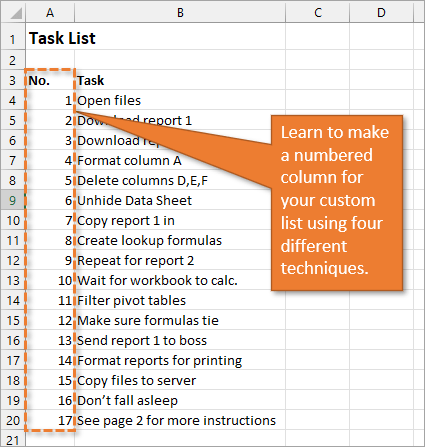
If you have a list of items in Excel and you’d like to insert a column that numbers the items, there are several ways to accomplish this. Let’s look at four of those ways.
1. Create a Static List Using Auto-Fill
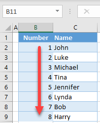
The first way to number a list is really easy. Start by filling in the first two numbers of your list, select those two numbers, and then hover over the bottom right corner of your selection until your cursor turns into a plus symbol. This is the fill handle.
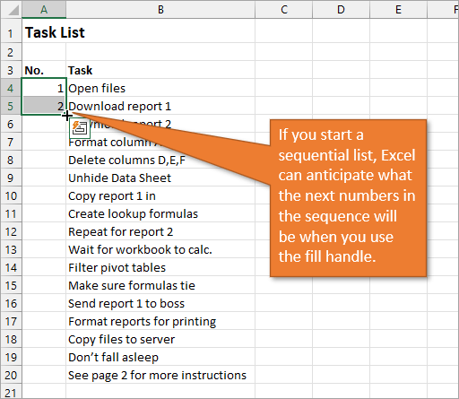
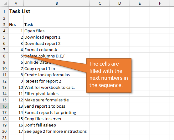
When you double-click on that fill handle (or drag it down to the end of your list), Excel will fill in the blanks with the next numbers in the sequence.
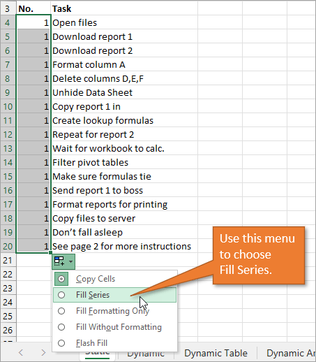
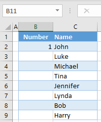
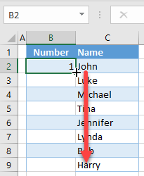
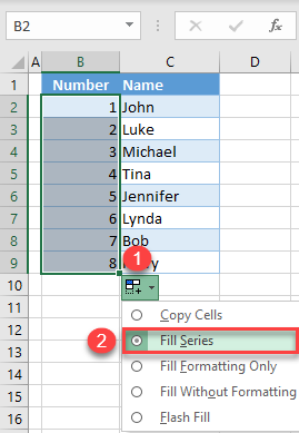
An alternate way to create this same numbered list is to type a 1 in the first cell and then double-click the fill handle. Because Excel doesn’t have a second number to identify a sequence or pattern, it will fill down the columns with 1s. But you will notice that a menu is available at the end of your column, and from that menu, you can select the option to Fill Series. This will change the 1s to a sequential list of numbers.
The numbered column we’ve created in both instances is static. This means it doesn’t change when you make additions or deletions to the corresponding list of items. For example, if I insert a new row in order to add another task, there is a break in the numbered column as well, and I would have to repeat the same steps to correct the list.
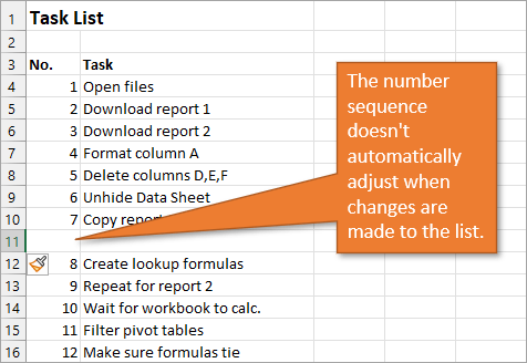
So, unless we want the numbers to always remain as they are, a better option would be to create a dynamic list.
2. Create a Dynamic List Using a Formula
We can use formulas to create a dynamic list where the numbers update when we add or delete rows from the list.
To use a formula for creating a dynamic number list, we can use the ROW function. The ROW function returns the row number of a cell. If we don’t specify a cell for ROW, it just returns the current row number of whatever is selected.
In our example, the first cell in our list doesn’t start on Row 1. It starts on Row 4. But we don’t want our list to start at 4; we want it to start at 1. To subtract the extra 3, our formula will include a minus sign and then the ROW function again, but this time pointed to the cell above our formula (which is in Row 3).
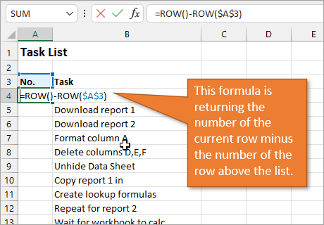
We use the absolute values (dollar signs) in our cell selection because we don’t want that number to change as we copy the formula down the list. In other words, we always want to subtract 3 from the row number to give us our list number.
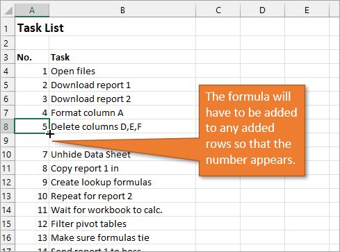
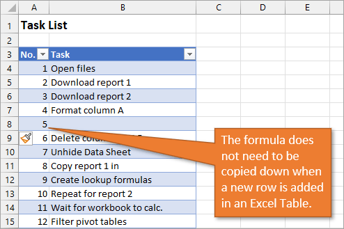
When we copy down the formula, we have a numbered list that will adjust when we add or delete rows. However, when adding a row, we will have to copy the formula into the newly inserted cell.
This additional step of copying the formula into new rows can be avoided if we use Excel Tables.
3. Create a Dynamic List Using a Formula in an Excel Table
If we write the same formula but we use an Excel table, the only difference we will make in the formula is that we reference the column header instead of the absolute cell value.
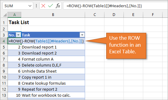
Because we are using an Excel Table, the formula automatically fills down to the other rows. When we add a row to the table, the formula will automatically populate in the new cell.
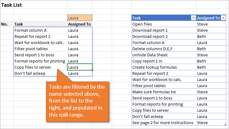
4. Create a Dynamic List Using Dynamic Array Formulas
Below, I have a table that is populated using Dynamic Array Formulas. The FILTER formula spills a range of results based on whatever name is selected in the orange cell.
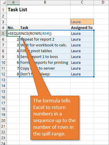
The Dynamic Array formula we will use is SEQUENCE. This will return a sequence for the number of rows we identify in the formula. To tell Excel how many rows there are, we will use the ROW function as the argument for sequence. The argument for ROW is just the spill range. The way to notate the spill range is to simply place a hashtag after the name of the first cell in the range. So our formula looks like this:
=SEQUENCE(ROWS(B5#))
Once we complete our formula and hit Enter, the list will be numbered.
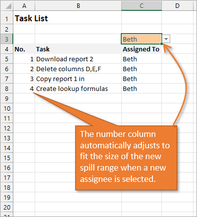
With this formula in place, if the size of the range changes when a new name is selected, the numbered column for the list will automatically adjust as well.
Bonus Tip: Formatting Your Numbered List
If you want to add periods or other punctuation to your numbered list:
- Select the entire list and right-click to choose Format Cells. Or use the keyboard shortcut Ctrl + 1.
- Choose the Custom option on the Number tab.
- Then in the Type field, type in the number 0 with whatever punctuation you would like to surround your number.
Here, I’ve just added a period.
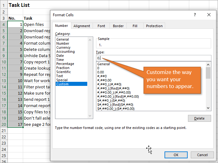
When you hit OK, you will have formatted the entire selection.
Related Posts
Here are a few similar posts that may interest you.
- Excel Tables Tutorial Video – Beginners Guide for Windows & Mac
- New Excel Features: Dynamic Array Formulas & Spill Ranges
- How to Prevent Excel from Freezing or Taking A Long Time when Deleting Rows
Conclusion
I hope these four ways to create ordered lists are helpful for you. If you have questions or feedback, I would love to hear them in the comments. Have a great week!
Содержание
- How to Make a List of Numbers in Excel & Google Sheets
- AutoFill Numbers
- Double-Click the Fill Handle
- Fill Command
- AutoFill Numbers in Google Sheets
- How to create a bulleted or numbered list in Microsoft Excel
- Create a bulleted or numbered list in Excel
- Add bulleted and numbered list option to the Ribbon
- Add a text box to a worksheet
- Add bulleted or numbered list to the text box
- Automatically number rows
- What do you want to do?
- Fill a column with a series of numbers
- Use the ROW function to number rows
- Display or hide the fill handle
- Add a list of numbers in a column
- Excel: Listing Numbers In Between 2 Numbers
- 3 Answers 3
How to Make a List of Numbers in Excel & Google Sheets
This tutorial demonstrates how to make a list of numbers in Excel and Google Sheets.
AutoFill Numbers
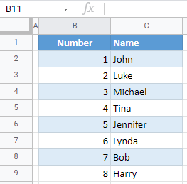
Say you have data in two columns in Excel. In Column C, there are names, while in Column B, you want to assign a number to each name, i.e., make a list of numbers in Column B.
Double-Click the Fill Handle
You can use AutoFill, by double-clicking, to populate cells based on the adjacent columns (non-blank columns to the left and right of the selected column). In this case, numbers are populated through Row 9.
- Enter 1 in cell B2. This is the initial data for Excel to recognize the pattern for AutoFill functionality.
- Position the cursor in the bottom-right corner of cell B2, and double-click the fill handle (the little black cross that appears).
- Click on AutoFill options and select Fill Series. Consecutive numbers are automatically populated through cell B9.
Fill Command
The above example could also be achieved using the Fill command on the Ribbon.
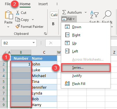
- Select the range of cells – including the initial value – where you want numbers populated (B2:B9). Then in the Ribbon, go to Home > Fill > Series.
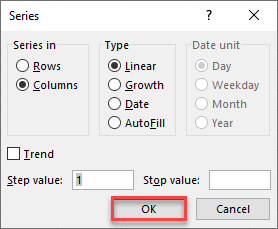
- In the pop-up screen, leave the default values: The column should be populated, and the Step value (increment) is 1. Press OK.
You get the same output: Numbers 1–8 fill cells B2:B9.
AutoFill Numbers in Google Sheets
You can also autofill numbers by double-clicking the fill handle (or just dragging it) in Google Sheets. Unlike in Excel, you need at least two numbers in Google Sheets to be able to recognize a pattern.
- Enter 1 in cell B2, and 2 in cell B3. This is the initial data for Google Sheets to recognize the pattern for AutoFill functionality.
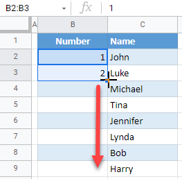
- Select cells B2 and B3, position the cursor in the bottom-right corner of cell B3, and double-click the fill handle.
As a result, a list of consecutive number is filled in Column B.
Источник
How to create a bulleted or numbered list in Microsoft Excel

A bulleted and numbered list is an available feature in Microsoft Excel, but not as commonly used as in word processing documents or presentation slides. By default, the bulleted and numbered lists option is hidden in Excel and must be added to the Ribbon. Additionally, a bulleted and numbered list cannot be added to a cell in Excel. A text box must be created, and then a bulleted or numbered list is added to that text box.
Create a bulleted or numbered list in Excel
Add bulleted and numbered list option to the Ribbon
- Open Microsoft Excel.
- Click the File tab in the Ribbon.
- Click Options in the left navigation menu.
- In the Excel Options window, click Customize Ribbon in the left navigation menu.
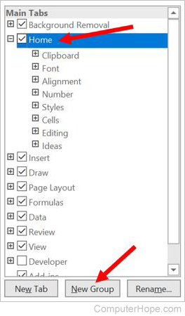
- On the right side of the Excel Options window, click the Home entry in the Main Tabs box.
- Click the New Group button below the Main Tabs box.
- A new group is added to the Home group. Click the New Group (Custom) entry, and click the Rename button.
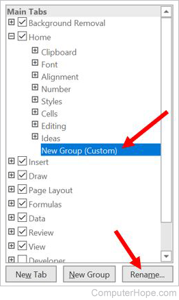
- Enter a new name, like Bullets or Bullet Lists, for the group.
- On the left side of the Excel Options window, click the Choose commands from drop-down list and select All Commands.
- In the list below, scroll down and find the Bullets and Numbering option. Click that entry and drag it to the new group you created on the right.
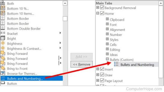
- Click the OK button to create the new group on the Home tab in the Ribbon, with the Bullets and Numbering option in it. The new group and option is found on the Home tab, on the far right side.
Add a text box to a worksheet
- Click the Insert tab in the Ribbon.
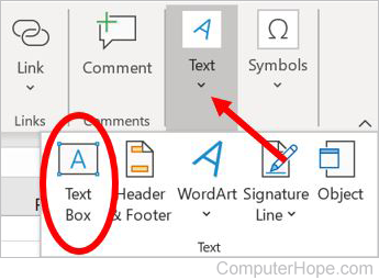
- On the Insert tab, click the Text option on the far right side, and select the Text Box option.
- In the worksheet, press and hold the left mouse button where you want to create the text box. Drag the mouse down and to the right, creating the text box with the desired size.
Add bulleted or numbered list to the text box
- Click in the text box you added to the worksheet.
- Click the Home tab in the Ribbon.
- Click the Bullets and Numbering option in the new group you created. The new group is on the far right side of the Home tab.
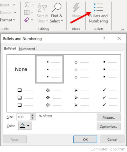
- In the Bullets and Numbering window, select the type of bulleted or numbered list you want to add to the text box and click OK.
- Type the text for each bullet point in the text box, pressing Enter to create the next bullet point.
- After entering the text for all desired bullet points, you can move the text box to any location in the worksheet. You can also resize the text box to better fit the bulleted or numbered list, if necessary.
Источник
Automatically number rows
Unlike other Microsoft 365 programs, Excel does not provide a button to number data automatically. But, you can easily add sequential numbers to rows of data by dragging the fill handle to fill a column with a series of numbers or by using the ROW function.
Tip: If you are looking for a more advanced auto-numbering system for your data, and Access is installed on your computer, you can import the Excel data to an Access database. In an Access database, you can create a field that automatically generates a unique number when you enter a new record in a table.

What do you want to do?
Fill a column with a series of numbers
Select the first cell in the range that you want to fill.
Type the starting value for the series.
Type a value in the next cell to establish a pattern.
Tip: For example, if you want the series 1, 2, 3, 4, 5. type 1 and 2 in the first two cells. If you want the series 2, 4, 6, 8. type 2 and 4.
Select the cells that contain the starting values.
Note: In Excel 2013 and later, the Quick Analysis button is displayed by default when you select more than one cell containing data. You can ignore the button to complete this procedure.
Drag the fill handle  across the range that you want to fill.
Note: As you drag the fill handle across each cell, Excel displays a preview of the value. If you want a different pattern, drag the fill handle by holding down the right-click button, and then choose a pattern.
To fill in increasing order, drag down or to the right. To fill in decreasing order, drag up or to the left.
Tip: If you do not see the fill handle, you may have to display it first. For more information, see Display or hide the fill handle.
Note: These numbers are not automatically updated when you add, move, or remove rows. You can manually update the sequential numbering by selecting two numbers that are in the right sequence, and then dragging the fill handle to the end of the numbered range.
Use the ROW function to number rows
In the first cell of the range that you want to number, type =ROW(A1).
The ROW function returns the number of the row that you reference. For example, =ROW(A1) returns the number 1.
Drag the fill handle across the range that you want to fill.
Tip: If you do not see the fill handle, you may have to display it first. For more information, see Display or hide the fill handle.
These numbers are updated when you sort them with your data. The sequence may be interrupted if you add, move, or delete rows. You can manually update the numbering by selecting two numbers that are in the right sequence, and then dragging the fill handle to the end of the numbered range.
If you are using the ROW function, and you want the numbers to be inserted automatically as you add new rows of data, turn that range of data into an Excel table. All rows that are added at the end of the table are numbered in sequence. For more information, see Create or delete an Excel table in a worksheet.
To enter specific sequential number codes, such as purchase order numbers, you can use the ROW function together with the TEXT function. For example, to start a numbered list by using 000-001, you enter the formula =TEXT(ROW(A1),»000-000″) in the first cell of the range that you want to number, and then drag the fill handle to the end of the range.
Display or hide the fill handle
The fill handle displays by default, but you can turn it on or off.
In Excel 2010 and later, click the File tab, and then click Options.
In Excel 2007, click the Microsoft Office Button  , and then click Excel Options.
In the Advanced category, under Editing options, select or clear the Enable fill handle and cell drag-and-drop check box to display or hide the fill handle.
Note: To help prevent replacing existing data when you drag the fill handle, ensure the Alert before overwriting cells check box is selected. If you do not want Excel to display a message about overwriting cells, you can clear this check box.
Источник
Add a list of numbers in a column
To quickly get a total instead of typing each number into a calculator.
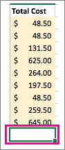
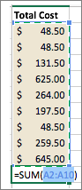
Click the first empty cell below a column of numbers.
Do one of the following:
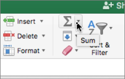
Excel 2016 for Mac: : On the Home tab, click AutoSum.
Excel for Mac 2011: On the Standard toolbar, click AutoSum.

Tip: If the blue border does not contain all of the numbers that you want to add, adjust it by dragging the sizing handles on each corner of the border.
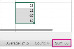
If you want a quick total that doesn’t have to appear on the sheet, select all the numbers in the list, and then look at the status bar at the bottom of the workbook window.
You can quickly insert the AutoSum formula by typing the  + SHIFT + T keyboard shortcut.
Источник
Excel: Listing Numbers In Between 2 Numbers
I was wondering if anyone knew of a formula to list all the numbers between 2 values, so for example if cell F2 had 12 in it and G2 had 17 in it I’d like a formula that would show 13,14,15,16 In cell H2.
3 Answers 3
This cannot be done with an Excel worksheet function. You will need VBA for that. It can be done with a user-defined function (UDF).
The following code needs to be stored in a code Module. You need to right-click the sheet tab, select View Code. This will open the Visual Basic Editor. Click Insert > Module and then paste the following code:
Now you can use a formula like =InBetween(F2,G2) to produce the result you describe.
You need to save the file as a macro-enabled workbook with the XLSM extension. See screenshot for code and user defined function in action.

Just because @teylyn said it couldn’t be done with a formula — here is a formula based solution:
First you need to create the full list of numbers that you are likely to need as a string, this could be in another cell or my preference would be to create a named range.
So create a new named range called rng and in the Refers to text box add the following formula:
For this solution to work you have to know the full range upfront, also note the leading and trailing comma.
Then enter the following formula into cell H2:
To same the tedium of creating the number range string I used the following Powershell code to create and copy it to the clipboard:
Just change the 20 in the above code for whatever range you require.
Источник
See all How-To Articles
This tutorial demonstrates how to make a list of numbers in Excel and Google Sheets.
AutoFill Numbers
Say you have data in two columns in Excel. In Column C, there are names, while in Column B, you want to assign a number to each name, i.e., make a list of numbers in Column B.
Double-Click the Fill Handle
You can use AutoFill, by double-clicking, to populate cells based on the adjacent columns (non-blank columns to the left and right of the selected column). In this case, numbers are populated through Row 9.
- Enter 1 in cell B2. This is the initial data for Excel to recognize the pattern for AutoFill functionality.
- Position the cursor in the bottom-right corner of cell B2, and double-click the fill handle (the little black cross that appears).
- Click on AutoFill options and select Fill Series. Consecutive numbers are automatically populated through cell B9.
Fill Command
The above example could also be achieved using the Fill command on the Ribbon.
- Select the range of cells – including the initial value – where you want numbers populated (B2:B9). Then in the Ribbon, go to Home > Fill > Series.
- In the pop-up screen, leave the default values: The column should be populated, and the Step value (increment) is 1. Press OK.
You get the same output: Numbers 1–8 fill cells B2:B9.
AutoFill Numbers in Google Sheets
You can also autofill numbers by double-clicking the fill handle (or just dragging it) in Google Sheets. Unlike in Excel, you need at least two numbers in Google Sheets to be able to recognize a pattern.
- Enter 1 in cell B2, and 2 in cell B3. This is the initial data for Google Sheets to recognize the pattern for AutoFill functionality.
- Select cells B2 and B3, position the cursor in the bottom-right corner of cell B3, and double-click the fill handle.
As a result, a list of consecutive number is filled in Column B.
Excel for Microsoft 365 for Mac Excel 2021 for Mac Excel 2019 for Mac Excel 2016 for Mac Excel for Mac 2011 More…Less
Why?
To quickly get a total instead of typing each number into a calculator.
How?
-
Click the first empty cell below a column of numbers.

-
Do one of the following:
-
Excel 2016 for Mac: : On the Home tab, click AutoSum.
-
Excel for Mac 2011: On the Standard toolbar, click AutoSum.
Tip: If the blue border does not contain all of the numbers that you want to add, adjust it by dragging the sizing handles on each corner of the border.
-
-
Press RETURN .
Tips:
-
If you want a quick total that doesn’t have to appear on the sheet, select all the numbers in the list, and then look at the status bar at the bottom of the workbook window.
-
You can quickly insert the AutoSum formula by typing the
+ SHIFT + T keyboard shortcut.
Need more help?
Updated: 02/01/2021 by
A bulleted and numbered list is an available feature in Microsoft Excel, but not as commonly used as in word processing documents or presentation slides. By default, the bulleted and numbered lists option is hidden in Excel and must be added to the Ribbon. Additionally, a bulleted and numbered list cannot be added to a cell in Excel. A text box must be created, and then a bulleted or numbered list is added to that text box.
Create a bulleted or numbered list in Excel
Add bulleted and numbered list option to the Ribbon
- Open Microsoft Excel.
- Click the File tab in the Ribbon.
- Click Options in the left navigation menu.
- In the Excel Options window, click Customize Ribbon in the left navigation menu.
- On the right side of the Excel Options window, click the Home entry in the Main Tabs box.
- Click the New Group button below the Main Tabs box.
- A new group is added to the Home group. Click the New Group (Custom) entry, and click the Rename button.
- Enter a new name, like Bullets or Bullet Lists, for the group.
- On the left side of the Excel Options window, click the Choose commands from drop-down list and select All Commands.
- In the list below, scroll down and find the Bullets and Numbering option. Click that entry and drag it to the new group you created on the right.
- Click the OK button to create the new group on the Home tab in the Ribbon, with the Bullets and Numbering option in it. The new group and option is found on the Home tab, on the far right side.
Add a text box to a worksheet
- Click the Insert tab in the Ribbon.
- On the Insert tab, click the Text option on the far right side, and select the Text Box option.
- In the worksheet, press and hold the left mouse button where you want to create the text box. Drag the mouse down and to the right, creating the text box with the desired size.
Add bulleted or numbered list to the text box
- Click in the text box you added to the worksheet.
- Click the Home tab in the Ribbon.
- Click the Bullets and Numbering option in the new group you created. The new group is on the far right side of the Home tab.
- In the Bullets and Numbering window, select the type of bulleted or numbered list you want to add to the text box and click OK.
- Type the text for each bullet point in the text box, pressing Enter to create the next bullet point.
- After entering the text for all desired bullet points, you can move the text box to any location in the worksheet. You can also resize the text box to better fit the bulleted or numbered list, if necessary.
This post will guide you how to filter only whole numbers from decimal numbers in a list in Excel. How do I filter cells with whole numbers or non-whole numbers in Excel.
Table of Contents
- List Only Whole Numbers
- Related Functions
Assuming that you have a list of data in range A1:A6, which contain decimal numbers and whole numbers. And you want to filter only the whole numbers or all non-whole numbers from the given list of data in Excel. You need to create a helper column next to the given data or range, and then using a formula based on INT function to check if the given number is integer or not. If return True, it indicates that this number is an integer or whole number. Otherwise, it is a non-whole number. Do the following steps:
#1 create a new column next to the numbers column, and type the following formula into cell B1.
=INT(A2)=A2
#2 press Enter key to apply this formula, and drag the AutoFill Handle down to other cells to apply this formula.
#3 select the helper column B, and go to DATA tab, click Filter button under Sort & Filter group. And one Filter icon added into the first cell in helper column.
#4 click filter icon in the Cell B1, and select TRUE or FALSE value as you what to filter out whole numbers or non-whole numbers. Click Ok button to apply for changes.
#5 you should see that all whole numbers have been filtered out . And if select FALSE option from the drop down list, and it will filtered out all decimal numbers.
Note: you can also use another formula based on the IF function and the MOD function to achieve the same result. Like this:
=IF(MOD(A1,1)<>0,0,A1)
Type this formula into Cell C2 in a help column, and press Enter key.
You should see that all whole numbers have been listed. And all decimal number will be shown as 0.
- Excel INT function
The Excel INT function returns the integer portion of a given number. And it will rounds a given number down to the nearest integer.The syntax of the INT function is as below:= INT (number)…
We know how to get the most frequently appearing number in excel. We use the MODE function. But if we want to list most frequently appearing numbers then this formula won’t work. We will be needing a combination of excel functions to do this task.
Here is the generic formula to list the most frequently occurring numbers:
numbers: This is the range or array from which we need to get the most frequently appearing numbers.
expanding_range: It is an expanding range that starts from one cell above where you write this formula. For example, if right the excel formula in the cell B4 then expanding rang will be $B$3:B3.
Now, let us see this formula in action.
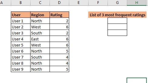
Example: Get 3 frequently appearing ratings.
So the scenario is this. We have some data on a survey in which users have rated our services. We need to get the 3 most frequently appearing ratings.
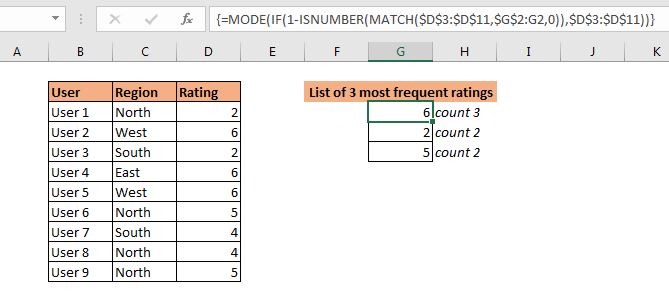
 Write this formula in G3:
This is an array formula. Use CTRL+SHIFT+ENTER. Drag down this formula in three cells. And now you have your 3 most frequently occurring numbers.
 Now that we have done it, let’s see how it is working.
How does it work?
Here the idea is to exclude already extracted most frequently appearing numbers in the next run of MODE function. to do so we use some extra help from other excel logical functions.
To understand it let’s have a look at the formula in cell G4. Which is:
The formula starts with the innermost function MATCH.
The MATCH function has lookup range D3:D11 (the numbers). The lookup value is also a range G2:G3 (expanded when copied down). Now, of course, G2 contains a text which is not in range D3:D11. Next, G3 contains 6. MATCH looks for 6 in range D3:D11 and returns an array of #N/A error and positions of 6 in range, which is {#N/A;2;#N/A;2;2;#N/A;#N/A;#N/A;#N/A}.
Now, this array is fed to the ISNUMBER function. ISNUMBER returns TRUE for numbers in the array. Hence we get another array as {FALSE;TRUE;FALSE;TRUE;TRUE;FALSE;FALSE;FALSE;FALSE}.
Next this array is subtracted from 1. As we know FALSE is treated as 0 and TRUE as 1. As we subtract this array from 1 we get an inverted array as {1;0;1;0;0;1;1;1;1}. This is the exact mirror image of the array returned by the ISNUMBER function.
Now, for each 1 (TRUE) MODE function runs. The MODE function gets an array {2;FALSE;2;FALSE;FALSE;5;4;4;5}. And finally, we get the most frequently appearing number in the array as 2. (Note that 5 and 4 both are occurring 2 times. But since 2 appeared first we get 2.
In G3, the ISNUMBER function returns an array of FALSE only. Hence the whole range is supplied to MODE function. Then mode function returns the most frequently appearing number in range as 6.
Another Formula
Another way is to use NOT function to invert the array return by ISNUMBER function.
So yeah guys, this how you can retrieve most frequently appearing numbers in excel. I hope I was explanatory enough. If you have any doubts regarding any function used in this formula, just click on them. It will take you to the explanation of that function. If you have any queries regarding this article or any other excel or VBA function, ask me in the comments section below.
Related Articles:
How to find frequently occurring numbers | Most frequently appearing numbers can be calculated using the MODE function of Excel.
Get most frequently appearing text in Excel | Learn how to get frequently appearing text in excel.
Lookup Frequently Appearing Text with Criteria in Excel | To get the most frequently appearing text in excel with criteria you just need to put an if condition before match function.
Retrieving the First Value in a List that is Greater / Smaller than a Specified Value | Learn how to lookup first value that is greater than a specified value. The generic formula to lookup is…
How to retrieve the entire row of a matched value| It is easy to look up and retrieve the entire row from a table. Let’s see how can we do this lookup.
How to Retrieve Latest Price in Excel | To look up the latest price from a range you must have your data sorted. Once sorted use this formula…
Popular Articles:
50 Excel Shortcuts to Increase Your Productivity | Get faster at your task. These 50 shortcuts will make you work even faster on Excel.
The VLOOKUP Function in Excel | This is one of the most used and popular functions of excel that is used to lookup value from different ranges and sheets.
COUNTIF in Excel 2016 | Count values with conditions using this amazing function. You don’t need filter your data to count specific value. Countif function is essential to prepare your dashboard.
How to Use SUMIF Function in Excel | This is another dashboard essential function. This helps you sum up values on specific conditions.
Excel Tips and Tutorials
Edit
Add to Favorites
Author: don
Excel Macro & VBA Course (80% Off)
Quickly create a large list of numbers in Excel using the Fill Command. This will save you time and allow you to create better spreadsheet models with less effort.
Steps to Create a Huge List of Numbers in Excel Quickly
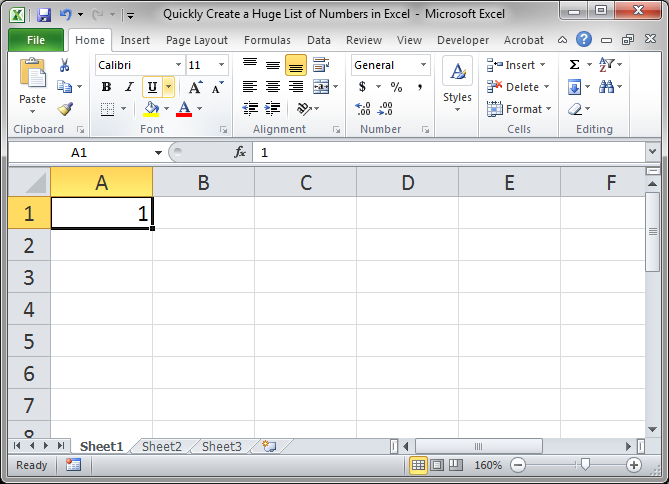
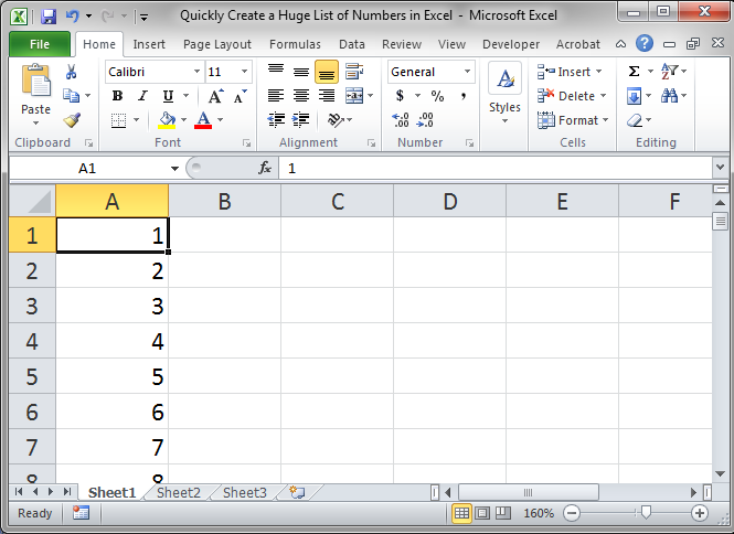
- Type the first number of the list that you want:
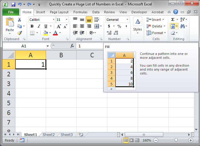
- Select that cell and go to the Home tab and then look to the right in the editing section and click the Fill button:
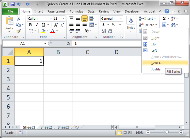
- Then click the Series… option:
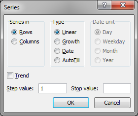
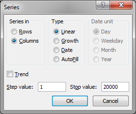
- A window will open and now you need to fill-in the options for your list:
Series in means if the list will go left and right in a single row (Rows option) or up and down in a single column (Columns option).
Type determines how the list will grow and, for this tutorial, we need to keep it at Linear so it will grow in a constant manner.
Step value says by how much you want each iteration of the list to grow. So, do you want each row to grow by 1 or 10 or 20 etc.
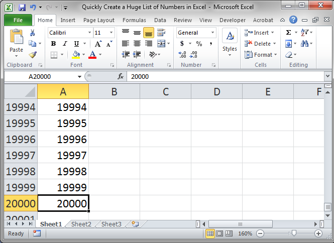
Stop Value is the number at which you want the list to stop. - We select Columns from the «Series in» section and keep the Step value at 1, so the numbers will increase by one each time, and then put 20000 in for the Stop value so the list will stop at 20000.
- Hit OK and then you have your list.
This may seem like a lot of steps but, once you understand what to do, it will take you no more than a few seconds to create a numbered list of any size and any interval.
Make sure to download the accompanying spreadsheet if you want to see this list.
Excel Version:
Excel 2007, Excel 2010, Excel 2013, Excel 2016
Downloadable Files:
Excel File
Sign-in to download the file.
![]()
Excel VBA Course — From Beginner to Expert
200+ Video Lessons
50+ Hours of Instruction
200+ Excel Guides
Become a master of VBA and Macros in Excel and learn how to automate all of your tasks in Excel with this online course. (No VBA experience required.)
View Course
Similar Content on TeachExcel
Require a Unique List of Numbers in a Range in Excel
Tutorial: I’ll show you how to require a user to enter a unique number into a range of cells in Exce…
Generate a Unique List of Random Numbers With a Simple Formula + (GUID/UUID Generator)
Tutorial:
Sections:
GUID/UUID V4 Formula in Excel
Versatile Formula to Generate a Unique List of N…
Format Cells as a Fraction in Excel Number Formatting
Macro: This free Excel macro will automatically format a selected cell or many selected cells in …
Keep Leading Zeros in Numbers in Excel — 2 Ways
Tutorial:
I’ll show you 2 ways to add and keep leading zeros in front of numbers in Excel.
These t…
Quickly Combine a List of Values and Put a Delimiter Between Each Value in Excel
Tutorial:
How to combine a list of data into one cell while putting a delimiter between each piece …
Convert Numbers Stored as Text to Numbers in Excel
Tutorial:
I’ll show you 4 ways to convert numbers stored as text to numbers in Excel. This situat…
Subscribe for Weekly Tutorials
BONUS: subscribe now to download our Top Tutorials Ebook!
Numbering in Excel means providing a cell with numbers like serial numbers to some table. We can also do it manually by filling the first two cells with numbers and dragging them down to the end of the table, which Excel will automatically load the series. Else, we can use the =ROW() formula to insert a row number as the serial number in the data or table.
When working with Excel, some small tasks need to be done repeatedly. However, if we know the right way to do it, they can save a lot of time. For example, generating the numbers in Excel is a task that is often used while working. Serial numbers play a very important role in Excel. It defines a unique identity for each record of your data.
One of the ways is to add the serial numbers manually in Excel. But it can be a pain if you have the data of hundreds or thousands of rows and must enter the row number for them.
This article will cover the different ways to do it.
Table of contents
- Numbering in Excel
- How to Add Serial Number in Excel Automatically?
- #1 – Using Fill Handle
- #2 – Using Fill Series
- #3 – Using the ROW Function
- Things to Remember about Numbering in Excel
- Recommended Articles
How to Add Serial Number in Excel Automatically?
There are many ways to generate the number of rows in Excel.
You can download this Numbering in Excel Template here – Numbering in Excel Template
- Using Fill Handle
- Using Fill Series
- Using ROW Function
#1 – Using Fill Handle
It identifies a pattern from a few already filled cells and then quickly uses that pattern to fill the entire column.
For example, let us take the below dataset.
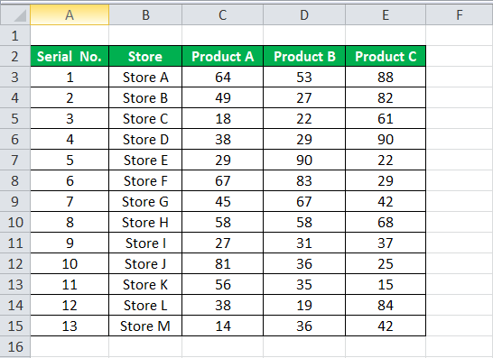
For the above dataset, we have to fill the serial no record-wise. Follow the below steps:
- First, we must enter 1 in cell A3 and insert 2 in cell A4.
- Then, select both the cells as per the below screenshot.

As we can see, a small square is shown in the above screenshot, which is rounded by a red color called “Fill Handle” in Excel.
Place the mouse cursor on this square and double-click on the fill handle.
- It will automatically fill all the cells until the end of the dataset. For example, refer to the below screenshot.

As the fill handle identifies the pattern, fill the individual cells with that pattern.
If you have any blank row in the dataset, the fill handle would only work until the last contiguous non-blank row.

#2 – Using Fill Series
It gives more control over data on how the serial numbers are entered into Excel.
For example, suppose you have below the score of students subject-wise.

Follow the below steps to fill series in the Excel:
- We must first insert 1 in cell A3.
- Then, go to the “HOME” tab. Next, click on the “Fill” option under the “Editing” section, as shown in the below screenshot.

- Click on the “Fill” dropdown. It has many options. Click on “Series,” as shown in the below screenshot.

- It will open a dialog box, as shown below screenshot.

- Click on “Columns” under the “Series in” section. Then, refer to the below screenshot.

- Insert the value under the “Stop value” field. In this case, we have 10 records; enter 10. If we skip this value, the Fill “Series” option may not work.
- Enter “OK.” It will fill rows with serial numbers from 1 to 10. Refer to the below screenshot.

#3 – Using the ROW Function
Excel has a built-in function, which also can be used to number the rows in Excel. To get the Excel row numbering, we must enter the following formula in the first cell shown below:

- The ROW function gives the Excel row number of the current row. We have subtracted 3 from it as we started the data from the 4th. If the data starts from the 2nd row, we must remove 1 from it.
- See the below screenshot. Using =ROW()-3 formula.

Drag this formula for the rest of the rows. The final result is shown below.
Using this formula for numbering will not damage the numbers if we delete a record in the dataset. Furthermore, since the ROW function does not reference cell addresses, it will automatically adjust to give the correct row number.
Things to Remember about Numbering in Excel
- The “Fill Handle” and “Fill Series” options are static. Therefore, if we move or delete any record or row in the dataset, the row number will not change accordingly.
- The ROW function gives the exact numbering if we cut and copy the data in Excel.
Recommended Articles
This article is a guide to Numbering in Excel. We discuss how to automatically add serial numbers in Excel using the fill handle, fill series, and ROW function, along with examples and downloadable templates. You may learn more about Excel functions from the following articles: –
- Auto Numbering in ExcelThere are two approaches for auto numbering. To begin, fill the first two cells with the series you wish to insert and drag it to the table’s end. Second, use the =ROW() formula to get the number, and then drag it to the table’s end.read more
- Row Limit in Excel
- Excel Negative NumberIn Excel, negative numbers, i.e. numbers less than 0 in value, are displayed with minus symbols by default.read more
- IsNumber FunctionISNUMBER function in excel is an information function that checks if the referred cell value is numeric or non-numeric.read more
- Null in ExcelNull is a type of error in Excel that occurs when two or more cell references provided in formulas are wrong, or when their position is incorrect. Using space in formulas between two cell references, for example, will result in a null error.read more
Reader Interactions