
When we need to collect data from others, they may write different things from their perspective. Still, we need to make all the related stories under one. Also, it is common that while entering the data, they make mistakes because of typo errors. For example, assume in certain cells, if we ask users to enter either “YES” or “NO,” one will enter “Y,” someone will insert “YES” like this, and we may end up getting a different kind of results. So in such cases, creating a list of values as pre-determined values allows the users only to choose from the list instead of users entering their values. Therefore, in this article, we will show you how to create a list of values in Excel.
Table of contents
- Create List in Excel
- #1 – Create a Drop-Down List in Excel
- #2 – Create List of Values from Cells
- #3 – Create List through Named Manager
- Things to Remember
- Recommended Articles
You can download this Create List Excel Template here – Create List Excel Template
#1 – Create a Drop-Down List in Excel
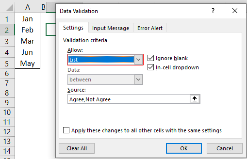
We can create a drop-down list in Excel using the “Data Validation in excelThe data validation in excel helps control the kind of input entered by a user in the worksheet.read more” tool, so as the word itself says, data will be validated even before the user decides to enter. So, all the values that need to be entered are pre-validated by creating a drop-down list in Excel. For example, assume we need to allow the user to choose only “Agree” and “Not Agree,” so we will create a list of values in the drop-down list.
- In the Excel worksheet under the “Data” tab, we have an option called “Data Validation” from this again, choose “Data Validation.”

- As a result, this will open the “Data Validation” tool window.
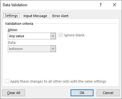
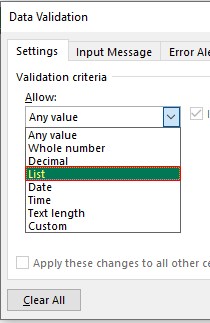
- The “Settings” tab will be shown by default, and now we need to create validation criteria. Since we are creating a list of values, choose “List” as the option from the “Allow” drop-down list.
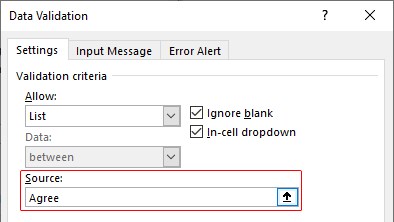
- For this “List,” we can give a list of values to be validated in the following way, i.e., by directly entering the values in the “Source” list.

- Enter the first value as “Agree.”
- Once the first value to be validated is entered, we need to enter “comma” (,) as the list separator before entering the next value. So, enter “comma” and enter the following values as “Not Agree.”
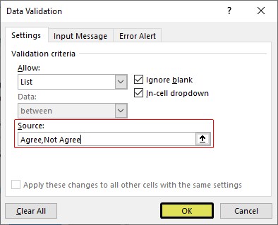
- After that, click on “Ok,” and the list of values may appear in the form of the “drop-down” list.

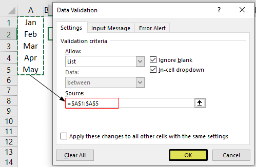
#2 – Create a List of Values from Cells
The above method is to get started, but imagine the scenario of creating a long list of values or your list of values changing now and then. Then, it may get difficult to return and edit the list of values manually. So, by entering values in the cell, we can easily create a list of values in Excel.
Follow the steps to create a list from cell values.
- We must first insert all the values in the cells.

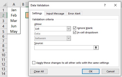
- Then, open “Data Validation” and choose the validation type as “List.”

- Next, in the “Source” box, we need to place the cursor and select the list of values from the range of cells A1 to A5.

- Click on “OK,” and we will have the list ready in cell C2.

So values to this list are supplied from the range of cells A1 to A5. Any changes in these referenced cells will also impact the drop-down list.
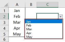
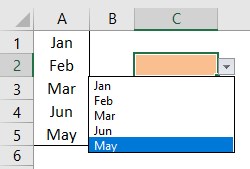
For example, in cell A4, we have a value as “Apr,” but now we will change that to “Jun” and see what happens in the drop-down list.
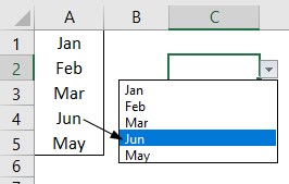
Now, look at the result of the drop-down list. Instead of “Apr,” we see “Jun” because we had given the list source as cell range, not manual entries.
#3 – Create List through Named Manager
There is another way to create a list of values, i.e., through named ranges in excelName range in Excel is a name given to a range for the future reference. To name a range, first select the range of data and then insert a table to the range, then put a name to the range from the name box on the left-hand side of the window.read more.
- We have values from A1 to A5 in the above example, naming this range “Months.”

- Now, select the cell where we need to create a list and open the drop-down list.
- Now place the cursor in the “Source” box and press the F3 key to an open list of named ranges.
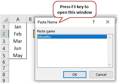
- As we can see above, we have a list of names, choose the name “Months” and click on “OK” to get the name to the “Source” box.
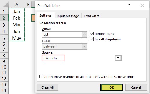
- Click on “OK,” and the drop-down list is ready.
Things to Remember
- The shortcut key to open data validation is “ALT + A + V + V.“
- We must always create a list of values in the cells so that it may impact the drop-down list if any change happens in the referenced cells.
Recommended Articles
This article has been a guide to Excel Create List. Here, we learn how to create a list of values in Excel also, create a simple drop-down method and make a list through name manager along with examples and downloadable Excel templates. You may learn more about Excel from the following articles: –
- Custom List in Excel
- Drop Down List in Excel
- Compare Two Lists in Excel
- How to Randomize List in Excel?
Microsoft Excel’s list function allows you to display several different values in a single cell using the form of a drop-down menu. When you activate the menu, you can view all of the values in the list. While the lists can be used as a space-saving convenience, they’re also useful in Excel forms when you want to make data entry easier or limit users to specific entries. You can populate your list with text, numbers or even formulas.
-
Open the worksheet where you want to create the list, and then open a new worksheet by clicking the «+» or the new worksheet icon at the bottom of the window.
-
Enter the values you want displayed in the list. The values should be in a single row or column on the new worksheet. Return to the original worksheet, and select the cell that will contain the list.
-
Select the «Data» tab, and then click «Data Validation» in the Data Tools section of the ribbon. The Data Validation dialog box appears.
-
Click the drop-down button next to «Allow,» and select «List» from the options. Make sure the box next to «In-cell Drop-down» is checked.
-
Click inside the «Source» field, and then switch to the worksheet containing the list values.
-
Select the range of cells containing the values. As you select the cells, the cell addresses automatically populate the «Source» field in the dialog box.
-
Click «OK» in the dialog box to create the list. Excel returns the focus to the original worksheet, and the cell containing the list has a new drop-down button. Click the button to view the list and select one of the values.

There are many scenarios you may come across while working in Excel where you only desire unique values in a list. You might want to rid your data of duplicates to create summaries, populate drop-down lists, or remove duplicates that found their way into your spreadsheet.
Luckily, Microsoft Excel offers many ways to accomplish summarizing values into a unique listing and depending on your particular situation, you may use different methods to accomplish the task at hand.
In this article, we’ll cover a bunch of different ways to identify those unique values so you have a full set of tactics to handle anything thrown your way. Let’s dive in!
1. Use The UNIQUE Function
With the release of Dynamic Array functions in 2020, Excel now offers a powerful function right out of the box to provide a simple way to pull together a list of unique values. Simply input the range you would like to analyze inside the UNIQUE Function and you’ll have the unique results delivered in a Spill Range below the formula.

If you’re looking for a more long-term solution, convert your data set into an Excel Table (ctrl + t) and point your UNIQUE function to read the table column. This will allow you to always have a more dynamic listing as your data grows or shrinks over time.

Pro Tip: If you want your list in alphabetical order add the Sort Function to your formula:
=SORT(UNIQUE(Table1[State]))
2. Use An Array Formula
Before the UNIQUE function was released, Excel users were left using more complex methods to compile a list of unique values from a range. Pretty much all of these methods involved using array formulas (think Ctrl+Shift+Enter) to output the end result. The formula I will share in this post does not require keying in Ctrl+Shift+Enter to activate it, hence why I prefer it. The downside to using an Array formula over an Dynamic Array function is you have to carry it down manually, there is no Spill Range functionality that will automatically resize your list.
I won’t go into the details of how this formula works (if interested go here), just know if you set it up properly it will magically work. Make sure you pay close attention to your dollar signs at the beginning of the COUNTIF function. It does matter that the first cell reference stays static while the other one changes as you carry the formula down (ie $G$3:G3 in the below example).
Finally, after you setup the first formula, you’ll need to drag the formula down until you start seeing #N/As. You’ll want to monitor your list if your data will be changing in the future to ensure it is picking up all the unique results. As a rule, I always make note to ensure at least one #N/A is showing at the bottom of my list.
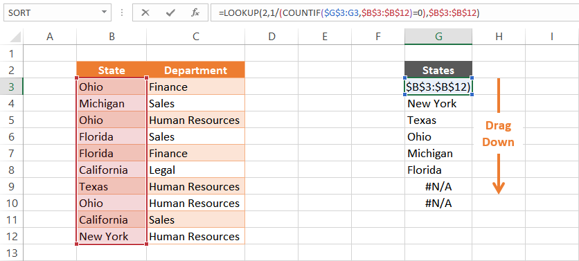
FORMULA: =LOOKUP(2,1/(COUNTIF($G$3:G3,$B$3:$B$12)=0),$B$3:$B$12)
3. Apply A Filter
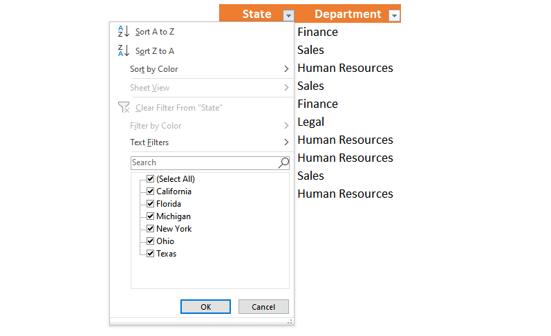
If you would like to see a list of unique values without necessarily needing to store the list, you can utilize a cell Filter (ctrl + shift + L). Apply a filter to your data and click the filter arrow to see a list showing all the unique values within that particular column of data.
4. Pivot Table
A Pivot Table is another good way to list out unique values. Select your data range (ensuring every column has a unique header value) and go to Insert > Pivot Table. When the Insert Dialog box appears , simply hit the OK button and you can start pivoting your data.
Drag the name of the column you would like to see a unique list of value for into the “Rows” quadrant. You should instantly see your list populate within the Pivot Table.
5. Remove Duplicates
If you actually want to modify your data so it only has unique values, you can utilize Excel’s Remove Duplicate button. This feature can be used on a range of cells or within an Excel Table.

Follow these steps to utilize this functionality:
-
Select your range of data
-
Navigate to the Data Ribbon tab.
-
Click the Remove Duplicates button within the Data Tools button group
-
Check the combination of columns you’d like to be unique

6. Highlight Duplicates With Conditional Formatting
You may run into situations where you want to quickly visualize if there are any duplicates in your data set. This is where you can apply a little bit of conditional formatting and luckily there is a preset to flag duplicate values!

Just follow these simple steps:
-
Highlight the cell range you want to analyze
-
Navigate to the Conditional Formatting button on the Home tab
-
Select Highlight Cells Rules
-
Select Duplicate Values…
-
Click OK

7. Use A Counting Formula
You might want to pursue utilizing a formula to flag your duplicate values. This can be done by using the COUNTIF() function. The below example shows how you can analyze each cell in the data range and understand if that value occurs more than once. If you have any count that is great than 1, you know there’s a duplicate within your data set.
Example Formula: =COUNTIF($D$4:$D$13, D4)
After you have implemented the formula, simply apply a filter and filter out all the “1” values.

If you are more concerned with having a duplicate row across multiple columns, you can add a helper column (Column D in the below example) that joins the values of the columns you want to ensure are unique. After the helper column is created, point your COUNTIF function to it and repeat the steps in the prior example.

Any Others I Missed?
Whew, that was a lot of techniques we went through to get to pretty much the same result. Hopefully, you start to realize as you find yourself needing to pull together a list of unique values, how valuable knowing all the options available to you in Excel. I’m sure there were other great methods that I overlooked or haven’t discovered yet. Please let me know if you have any tips in the comments section and I can growth this article even further!
I Hope This Helped!
Hopefully, I was able to explain how you can use a variety of methods to create unique lists of your data. If you have any questions about this technique or suggestions on how to improve it, please let me know in the comments section below.
About The Author
Hey there! I’m Chris and I run TheSpreadsheetGuru website in my spare time. By day, I’m actually a finance professional who relies on Microsoft Excel quite heavily in the corporate world. I love taking the things I learn in the “real world” and sharing them with everyone here on this site so that you too can become a spreadsheet guru at your company.
Through my years in the corporate world, I’ve been able to pick up on opportunities to make working with Excel better and have built a variety of Excel add-ins, from inserting tickmark symbols to automating copy/pasting from Excel to PowerPoint. If you’d like to keep up to date with the latest Excel news and directly get emailed the most meaningful Excel tips I’ve learned over the years, you can sign up for my free newsletters. I hope I was able to provide you some value today and hope to see you back here soon! — Chris
Create or delete a custom list for sorting and filling data
Excel for Microsoft 365 Excel 2021 Excel 2019 Excel 2016 Excel 2013 Excel 2010 Excel 2007 More…Less
Use a custom list to sort or fill in a user-defined order. Excel provides day-of-the-week and month-of-the year built-in lists, but you can also create your own custom list.
To understand custom lists, it is helpful to see how they work and how they are stored on a computer.
Comparing built-in and custom lists
Excel provides the following built-in, day-of-the-week, and month-of-the year custom lists.
|
Built-in lists |
|
Sun, Mon, Tue, Wed, Thu, Fri, Sat |
|
Sunday, Monday, Tuesday, Wednesday, Thursday, Friday, Saturday |
|
Jan, Feb, Mar, Apr, May, Jun, Jul, Aug, Sep, Oct, Nov, Dec |
|
January, February, March, April, May, June, July, August, September, October, November, December |
Note: You cannot edit or delete a built-in list.
You can also create your own custom list, and use them to sort or fill. For example, if you want to sort or fill by the following lists, you’ll need to create a custom list, since there is no natural order.
|
Custom lists |
|
High, Medium, Low |
|
Large, Medium, and Small |
|
North, South, East, and West |
|
Senior Sales Manager, Regional Sales Manager, Department Sales Manager, and Sales Representative |
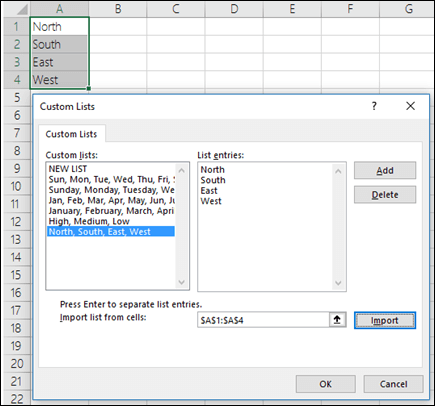
A custom list can correspond to a cell range, or you can enter the list in the Custom Lists dialog box.
Note: A custom list can only contain text or text that is mixed with numbers. For a custom list that contains numbers only, such as 0 through 100, you must first create a list of numbers that is formatted as text.
There are two ways to create a custom list. If your custom list is short, you can enter the values directly in the popup window. If your custom list is long, you can import it from a range of cells.
Enter values directly
Follow these steps to create a custom list by entering values:
-
For Excel 2010 and later, click File > Options > Advanced > General > Edit Custom Lists.
-
For Excel 2007, click the Microsoft Office Button
 > Excel Options > Popular >Top options for working with Excel > Edit Custom Lists.
 -
In the Custom Lists box, click NEW LIST, and then type the entries in the List entries box, beginning with the first entry.
Press the Enter key after each entry.
-
When the list is complete, click Add.
The items in the list that you have chosen will appear in the Custom lists panel.
-
Click OK twice.
 > Excel Options > Popular >Top options for working with Excel > Edit Custom Lists.
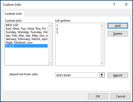
Create a custom list from a cell range
Follow these steps:
-
In a range of cells, enter the values that you want to sort or fill by, in the order that you want them, from top to bottom. Select the range of cells you just entered, and follow the previous instructions for displaying the Edit Custom Lists popup window.
-
In the Custom Lists popup window, verify that the cell reference of the list of items that you have chosen appears in the Import list from cells field, and then click Import.
-
The items in the list that you have chosen will appear in the Custom Lists panel.
-
Click OK twice.
Note: You can only create a custom list according to values, such as text, numbers, dates or times. You cannot create a custom list for formats such as cell color, font color, or an icon.
Follow these steps:
-
Follow the previous instructions for displaying the Edit Custom Lists dialog.
-
In the Custom Lists box, choose the list that you want to delete, and then click Delete.
Once you create a custom list, it is added to your computer registry, so that it is available for use in other workbooks. If you use a custom list when sorting data, it is also saved with the workbook, so that it can be used on other computers, including servers where your workbook might be published to Excel Services and you want to rely on the custom list for a sort.
However, if you open the workbook on another computer or server, you do not see the custom list that is stored in the workbook file in the Custom Lists popup window that is available from Excel Options, only from the Order column of the Sort dialog box. The custom list that is stored in the workbook file is also not immediately available for the Fill command.
If you prefer, add the custom list that is stored in the workbook file to the registry of the other computer or server and make it available from the Custom Lists popup window in Excel Options. From the Sort popup window, in the Order column, select Custom Lists to display the Custom Lists popup window, then select the custom list, and then click Add.
Need more help?
You can always ask an expert in the Excel Tech Community or get support in the Answers community.
Need more help?
 When you are working with large data sets, Excel’s built-in filters are a lifesaver, letting you get straight to the sub-set of data that you need. Sometimes, though, you need to be able to pull a set of data dynamically based on criteria that change. When the filter conditions change often, Excel’s filters fall short. Instead, there is a set of functions that can extract a data table from a larger data set based on specific criteria that you set. This tutorial will show you how to list values from a table based on filter criteria using sub-arrays and the SMALL function.
NOTE: The following article is a thorough breakdown of the individual pieces of a complicated array formula in Excel. If you just want to cut to the chase and look at the actual code, click the Using the Sub-Array Formula link in the table of contents.
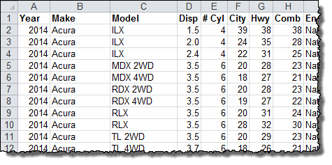
Example Data
For this exercise, we are going to use the 2014 auto fuel economy data from the EPA. This is the same data set used in the VLOOKUP with multiple criteria tutorial. In that exercise, we wanted to identify the fuel economy of a specific vehicle. Now, we are going to try to list all the vehicles that meet a minimum miles per gallon (MPG) rating.
The data is organized by Make, Model, Engine Displacement, Number of Cylinders, and the MPG ratings for City, Highway, and Combined mileage.
Get the latest Excel tips and tricks by joining the newsletter!
 Andrew Roberts has been solving business problems with Microsoft Excel for over a decade. Excel Tactics is dedicated to helping you master it.
Join the newsletter to stay on top of the latest articles. Sign up and you’ll get a free guide with 10 time-saving keyboard shortcuts!