
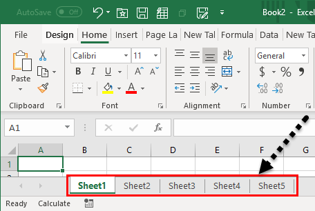
Where are my worksheet tabs?
Excel for Microsoft 365 Excel 2021 Excel 2019 Excel 2016 Excel 2013 Excel 2010 More…Less
If you can’t see the worksheet tabs at the bottom of your Excel workbook, browse the table below to find the potential cause and solution.
Note: The image in this article are from Excel 2016. Your view might be slightly different if you have a different version, but the functionality is the same (unless otherwise noted).
|
Cause |
Solution |
|---|---|
|
The window sizing is keeping the tabs hidden. |
If you still don’t see the tabs, click View > Arrange All > Tiled > OK. |
|
The Show sheet tabs setting is turned off. |
First ensure that the Show sheet tabs is enabled. To do this,
|
|
The horizontal scroll bar obscures the tabs. |
Hover the mouse pointer at the edge of the scrollbar until you see the double-headed arrow (see the figure). Click-and-drag the arrow to the right, until you see the complete tab name and any other tabs. |
|
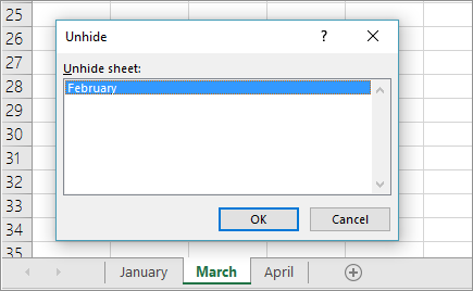
The worksheet itself is hidden. |
To unhide a worksheet, right-click on any visible tab and then click Unhide. In the Unhide dialog box, click the sheet you want to unhide and then click OK. |
Need more help?
You can always ask an expert in the Excel Tech Community or get support in the Answers community.
Need more help?
See all How-To Articles
This tutorial demonstrates how to view a list of worksheet tabs in Excel and Google Sheets.
View List of Worksheets
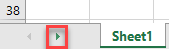
At the bottom of an Excel file, you can see tabs representing each sheet. When there’s a lot of sheets in a document, not all of the tabs can be displayed at once. In the following example, there are 20 worksheets, but only 7 of them are visible.
- To see the whole list of worksheets, right-click the arrow to the left of the sheet tabs.
![]()
All worksheet names are displayed in the pop-up list.
- To jump to a certain sheet, select the sheet’s name (e.g., Sheet5) and click OK.
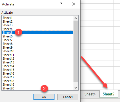
Cell A1 in Sheet5 is now selected.
View List of Worksheets in Google Sheets
- In Google Sheets, you can see the list of worksheets by clicking on the All Sheets icon to the left of the tabs.
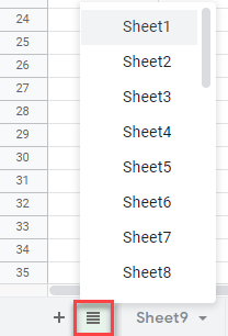
- If you scroll through the list, you can see all sheet names. As in Excel, clicking on a sheet’s name leads you to that sheet.
See also: How to Rename a Worksheet, How to Search All Sheets, and List Sheet Names with Formula.
Содержание
- Where are my worksheet tabs?
- Need more help?
- How to View List of Worksheet Tabs in Excel & Google Sheets
- View List of Worksheets
- View List of Worksheets in Google Sheets
- Why Can’T I See Tabs In Excel?
- How do I show all tabs in Excel?
- Why can I not unhide tabs in Excel?
- How do I restore tabs in Excel?
- How do you show hidden tabs in Excel?
- How do you get tabs back?
- How do I show all tabs?
- Why is hide sheet greyed out?
- How do I see closed tabs?
- What happened closed tab reopen?
- Why is reopen closed tab gone?
- How do I show all tabs in Windows?
- How do you add a tab in an Excel tab?
- What are tabs in Microsoft Excel?
- How do I unhide a greyed out cell in Excel?
- How do I unhide the GREY area in Excel?
- How do you undo closing all tabs?
- How do I reopen a closed window?
- How do I reopen a closed window in Windows 10?
- How do you get tabs back on a Mac?
- How do I open a tab?
- See All Sheets/Tabs In Excel/Go To A Sheet/Tab In Excel Quickly
- How to Show Sheet Tabs in Excel
- Turn On Show Sheet Tabs Settings
- Unhide the Worksheet(s)
- Instant Connection to an Expert through our Excelchat Service
Where are my worksheet tabs?
If you can’t see the worksheet tabs at the bottom of your Excel workbook, browse the table below to find the potential cause and solution.
Note: The image in this article are from Excel 2016. Your view might be slightly different if you have a different version, but the functionality is the same (unless otherwise noted).
The window sizing is keeping the tabs hidden.
If you restore multiple windows in Excel, ensure that the windows are not overlapping. Perhaps the top of an Excel window is covering the worksheet tabs of another window.
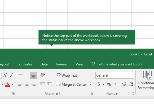
The status bar has been moved all the way up to the Formula Bar.
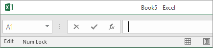
Tabs can also disappear if your computer screen resolution is higher than that of the person who last saved the workbook.
Try maximizing the window to reveal the tabs. Simply double-click the window title bar.
If you still don’t see the tabs, click View > Arrange All > Tiled > OK.
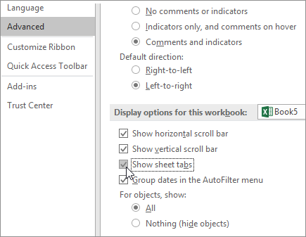
The Show sheet tabs setting is turned off.
First ensure that the Show sheet tabs is enabled. To do this,
For all other Excel versions, click File > Options > Advanced—in under Display options for this workbook—and then ensure that there is a check in the Show sheet tabs box.
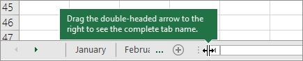
The horizontal scroll bar obscures the tabs.
Hover the mouse pointer at the edge of the scrollbar until you see the double-headed arrow (see the figure). Click-and-drag the arrow to the right, until you see the complete tab name and any other tabs.
The worksheet itself is hidden.
To unhide a worksheet, right-click on any visible tab and then click Unhide. In the Unhide dialog box, click the sheet you want to unhide and then click OK.
Need more help?
You can always ask an expert in the Excel Tech Community or get support in the Answers community.
Источник
How to View List of Worksheet Tabs in Excel & Google Sheets
This tutorial demonstrates how to view a list of worksheet tabs in Excel and Google Sheets.
View List of Worksheets
At the bottom of an Excel file, you can see tabs representing each sheet. When there’s a lot of sheets in a document, not all of the tabs can be displayed at once. In the following example, there are 20 worksheets, but only 7 of them are displayed.
To see the whole list of worksheets, right-click the arrow to the left of the sheet tabs.
All worksheet names are displayed in the pop-up list.
To jump to a certain sheet, select the sheet’s name (e.g., Sheet5), and click OK.
Cell A1 in Sheet5 is now selected.
View List of Worksheets in Google Sheets
In Google Sheets, you can see the list of worksheets by clicking on the All Sheets icon to the left of the tabs.
If you scroll through the list, you can see all sheet names. As in Excel, clicking on a sheet’s name leads you to that sheet.
Источник
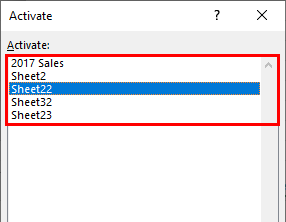
Why Can’T I See Tabs In Excel?
First ensure that the Show sheet tabs is enabled. To do this, For all other Excel versions, click File > Options > Advanced—in under Display options for this workbook—and then ensure that there is a check in the Show sheet tabs box.
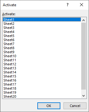
How do I show all tabs in Excel?
Excel: Right Click to Show a Vertical Worksheets List
- Right-click the controls to the left of the tabs.
- You’ll see a vertical list displayed in an Activate dialog box. Here, all sheets in your workbook are shown in an easily accessed vertical list.
- Click on whatever sheet you need and you’ll instantly see it!
Why can I not unhide tabs in Excel?
If the workbook contains only very hidden sheets, you won’t even be able to open the Unhide dialog box because the Unhide command will be disabled. If the workbook contains both hidden and very hidden sheets, the Unhide dialog will be available, but very hidden sheets won’t be listed there.
How do I restore tabs in Excel?
How to undo/restore deleted worksheets in Excel?
- Open the folder which contains the current workbook with right clicking this workbook’s tab and selecting the Open Folder from the right-clicking menu.
- Go back to Excel and click File (or Office button) > Save As.
If you want to see just one or two hidden sheets, here’s how you can quickly unhide them:
- In your Excel workbook, right-click any sheet tab and select Unhide… from the context menu.
- In the Unhide box, select the hidden sheet you want to display and click OK (or double-click the sheet name). Done!
How do you get tabs back?
You can simply right-click an empty area in the tab bar section and choose reopen closed tabs. You can also use a keyboard shortcut — press Ctrl+Shift+T (or Command+Shift+T on a Mac) and the last tab you closed will reopen in a new tab page.
How do I show all tabs?
As of 2021, there is a native Chrome feature that allows you to scroll through all of your open chrome tabs (as well as some recently closed ones). To access it, click on the dropdown arrow next to the minimize tab button. It will open up a scrollable dropdown with all tabs open in Chrome.
Why is hide sheet greyed out?
When the Very Hidden attribute is set on a worksheet, the Hide option is greyed out. Very hidden sheets can only be made visible through the VBA editor. If you want to unhide a very hidden sheet, open the VBA editor and change the Visible attribute back to xlSheetVisible.
How do I see closed tabs?
You can also press Ctrl+Shift+T on your keyboard to reopen the last closed tab. Repeatedly selecting “Reopen closed tab”, or pressing Ctrl+Shift+T will open previously closed tabs in the order they were closed.
What happened closed tab reopen?
You can use the Ctrl + Shift + T shortcut to reopen recently closed tabs.
Why is reopen closed tab gone?
You need to point the cursor on the empty header bar where tabs are not present. From the list, you can view and select the option Reopen Closed Tab. This is where the command has now moved and stays in the future. Alternatively, you can also lookup for recently closed tabs under the history tab.
How do I show all tabs in Windows?
In Settings, click “System,” then select “Multitasking” from the sidebar. In Multitasking settings, locate the “Pressing Alt + Tab shows” drop-down menu and click it. When the menu appears, select “Open windows and all tabs in Edge.”
How do you add a tab in an Excel tab?
Hold down [Shift] and click the first and last sheet tabs to create a contiguous group (Figure A). You’ll notice that the tabs change color when grouped. Use [Ctrl] to click individual tabs to create a group of noncontiguous sheets.
What are tabs in Microsoft Excel?
In Microsoft Excel, a sheet, sheet tab, or worksheet tab is used to display the worksheet that a user is currently editing. By clicking a worksheet tab (located at the bottom of the window), users may move between the various worksheets. Every Excel file may have multiple worksheets, but the default number is three.
How do I unhide a greyed out cell in Excel?
Replies (4)
- CTRL+A to select entire worksheet.
- Right click on any row number and take unhide.
- Right click on any column number and take unhide.
How do I unhide the GREY area in Excel?
You may also perform the steps below:
- Use Alt+F11 to go to the VBA Editor.
- Open the Project-Explorer (Ctrl+R) and select the appropriate worksheet.
- Open the Properties window (F4) select the property Visible and change it to xlSheetVisible .
How do you undo closing all tabs?
Reopen Recent Tabs in Chrome Android
- Open the Chrome on the Android app.
- Tap on. for more options.
- Select Recent tabs from the list.
- Here you will be able to see all the Recently closed websites.
- Tap on the Website that you want to reopen.
How do I reopen a closed window?
You can also press Ctrl+Shift+T on Windows or Cmd+Shift+T on Mac to reopen a closed tab with a keyboard shortcut. If you recently closed a window, this will reopen the closed window instead.
How do I reopen a closed window in Windows 10?
Press Ctrl + Shift + F to reopen the recently closed folders. If you don’t need to open the most recently closed program or folder, but another one listed on the UndoClose window, don’t press the hotkeys. You can open a listed program or folder on the window by clicking it instead.
How do you get tabs back on a Mac?
You can use the keyboard shortcut Shift + Command + T to reopen your last closed tab. This works no matter what you have open in your browser. You can also reopen a closed tab with the keyboard shortcut Command + Z. This makes the last closed tab reappear in the same spot where it last was among your open tabs.
How do I open a tab?
Open a new tab on Android tablet
- On your Android tablet, open the Chrome app .
- At the top, next to your open tabs, tap New tab .
Источник
See All Sheets/Tabs In Excel/Go To A Sheet/Tab In Excel Quickly
This post demonstrates how could we quickly see all available sheets in excel and navigate directly to any sheet in excel without going through all the sheets.
Sometimes we work with excel workbooks which has a large number of sheets and navigating between them is not a very efficient task if we have to do it sequentially, in this case we would require an efficient way to directly jump to a particular sheet by seeing all the available tabs in excel workbook.
Below is a pic an which shows a workbook that has 12 worksheets (not all of them visible though) and what if I want to go to sheet 3 directly from sheet 12, time taking isn’t it?

We will discuss a simple technique here by which you could easily see all the sheets/tabs in the workbook and you could go to any of them directly without having to scroll to it individually.
To see all the sheets/tabs and go to any sheets/tabs directly just right click anywhere over the arrow icons at the leftmost part of sheet names as shown in the pic below.

As you could see in the pic above, all the sheets/tabs are listed in quick way and you could go to any sheets/tabs simply just by clicking on them.
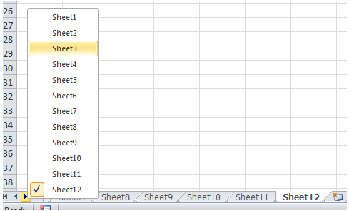
Here in the pic above I have shown you how to navigate directly to Sheet 3 from Sheet 12 in excel.
Источник
How to Show Sheet Tabs in Excel
When we open the Excel workbook, it contains several worksheet tabs like Sheet1, Sheet2, Sheet3 or the named worksheet tab like January, February, etc. Sometimes, we can’t see tabs , some or all of them, at the bottom of the workbook. We need to learn methods of how to make these sheet tabs visible when not showing tabs .
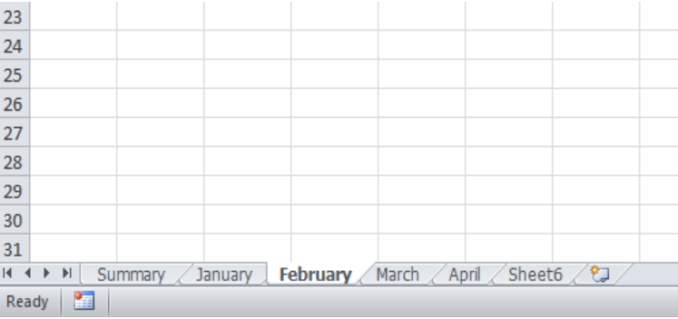 Figure 1. How to Show Tabs
Turn On Show Sheet Tabs Settings
If none of the worksheet tabs is visible at the bottom of the workbook, then it means Show Sheet Tabs settings is turned off. Therefore, we must check the settings and ensure to make it turned on to show tabs by following the below steps;
- Go to File and select Excel Options .
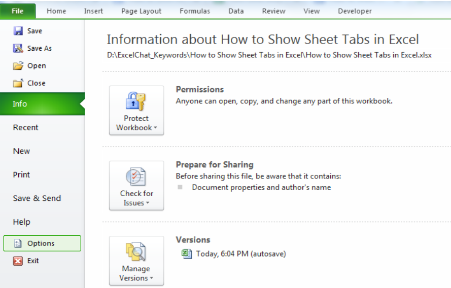 Figure 2. Excel Options
- On the left side of the Options window, select Advanced settings and scroll it down. Under the Display options for this workbook , make sure that there is check (⇃) on Show Sheet Tabs checkbox. Turn it on if it is not selected.
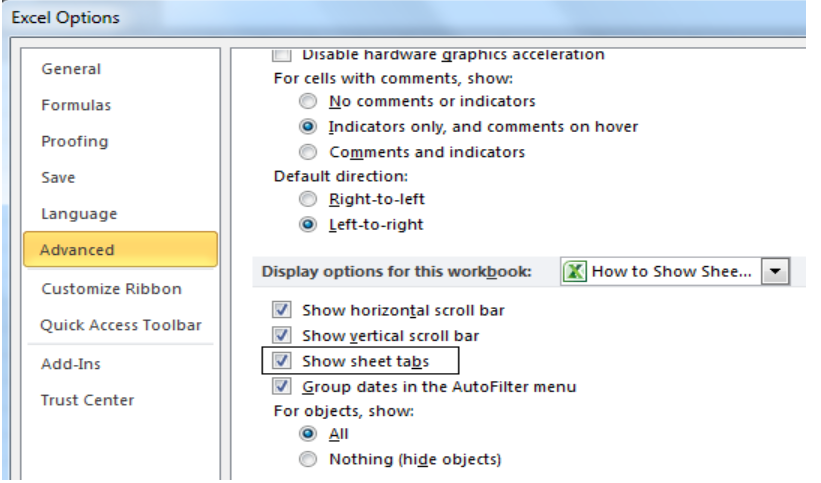 Figure 3. Show Sheet Tabs Settings
Unhide the Worksheet(s)
If some of the worksheets are not displaying then it means that they are either hidden or there is an issue with Excel not showing tabs .
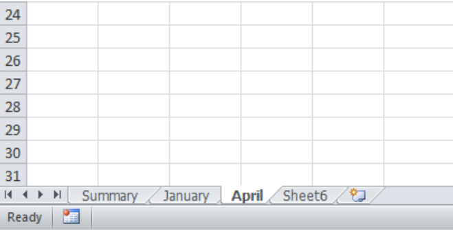 Figure 4. Can’t See Tabs
We need to make hidden worksheet(s) unhidden by following these steps;
- Right-click on any of the visible sheet tabs and select Unhide
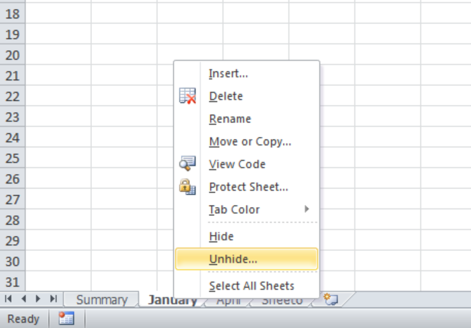 Figure 5. Unhide Sheet tabs
- From the Unhide dialog box, select the hidden sheet tab(s) and press the OK button.
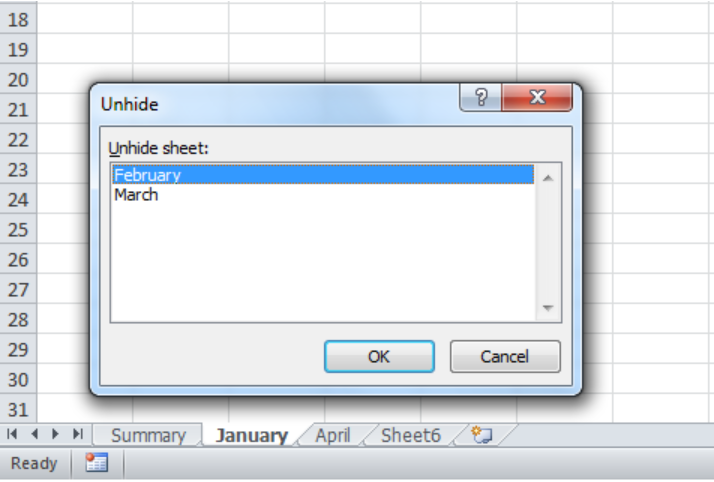 Figure 6. Hidden Sheet Tabs
- After unhiding all the tabs not showing , we can view tabs now.
 Figure 7. Unhiding Worksheets
Instant Connection to an Expert through our Excelchat Service
Most of the time, the problem you will need to solve will be more complex than a simple application of a formula or function. If you want to save hours of research and frustration, try our live Excelchat service! Our Excel Experts are available 24/7 to answer any Excel question you may have. We guarantee a connection within 30 seconds and a customized solution within 20 minutes.
Источник
Assume an MS Excel file has 4 worksheets – Sheet1, Sheet2, Sheet3 and Sheet4. Insert a sheet before Sheet1 and name that tab as Summary. On the Summary tab, one may want to generate a list of all sheet names from cell C7 onwards. Furthermore, the sheet names so generated, should be dynamic for the following changes:
1. Sheets added
2. Sheets deleted
3. Sheets renamed
4. Sheets repositioned
While this can be accomplished by using VBA, you may refer to my formula based solution here.
To generate a list of all Excel files in a specific folder, you may refer to the following post.
Table of Contents
- 1 How do you get a list of all tabs in an Excel workbook?
- 2 How many tabs can I create in Excel?
- 3 How do I automatically rename a sheet in Excel?
- 4 Why we Cannot name history on Excel work sheet?
- 5 Why is it important to rename a sheet?
- 6 How does excel name new worksheets quizlet?
- 7 How many new worksheets can you add to an Excel workbook quizlet?
- 8 How do you create a workbook in Excel?
- 9 How do you create a blank workbook in Excel?
- 10 How do you insert data into a cell phone?
- 11 How do I corrupt an Excel file?
How do you get a list of all tabs in an Excel workbook?
Excel: Right Click to Show a Vertical Worksheets List
- Right-click the controls to the left of the tabs.
- You’ll see a vertical list displayed in an Activate dialog box. Here, all sheets in your workbook are shown in an easily accessed vertical list.
- Click on whatever sheet you need and you’ll instantly see it!
How many tabs can I create in Excel?
255 sheets
How do you name a sheet in Excel?
Rename a worksheet
- Double-click the sheet tab, and type the new name.
- Right-click the sheet tab, click Rename, and type the new name.
- Use the keyboard shortcut Alt+H > O > R, and type the new name.
How do I automatically rename a sheet in Excel?
We can quickly rename worksheets in Excel with the Rename command according to the following procedures: Right click on the sheet tab you want to rename, and choose Rename command from the Right-click menu. Or double click on the sheet tab to rename the worksheet.
Why we Cannot name history on Excel work sheet?
History is a reserved name for the sheet meant for ‘tracking changes between shared workbooks’. A dialog called Highlight Changes will be activated. Mark the check box against ‘Track changes while editing’ and click OK. You will have a worksheet called History with the list of changes made in the workbook.
What character are not allowed in sheet names?
The name must be unique within a single workbook. A worksheet name cannot exceed 31 characters. You can use all alphanumeric characters but not the following special characters: , / , * , ? , : , [ , ].
Why is it important to rename a sheet?
The sheet names can be changed so that they explain what is contained within a particular sheet. It is also possible to change the color of each tab. There are three ways that a new sheet can be added to a workbook.
How does excel name new worksheets quizlet?
Terms in this set (38)
- double-click the sheet tab or right-click the worksheet tab and select rename.
- excel highlights the sheet name.
- type the new sheet name, and press enter.
What are the three ways to view a worksheet?
Excel offers three workbooks views, Normal, Page Layout and Page Break Preview.
How many new worksheets can you add to an Excel workbook quizlet?
1) A workbook can have at most 3 worksheets.
How do you create a workbook in Excel?
Open a new, blank workbook
- Click the File tab.
- Click New.
- Under Available Templates, double-click Blank Workbook. Keyboard shortcut To quickly create a new, blank workbook, you can also press CTRL+N.
What is difference between workbook and worksheet?
Workbook is an excel file containing many worksheets. A worksheet has a single spreadsheet containing data. 2. Workbook cannot be added within the worksheet.
How do you create a blank workbook in Excel?
Newer versions such as Excel 2016 will take you to a menu called backstage view to choose to open a new blank workbook or open a new workbook from a template. If you already have a file open in Excel, you can create a new document by clicking File>New. You can also use the shortcut Ctrl+N (Command+N for Mac).
How do you insert data into a cell phone?
Enter text or a number in a cell
- On the worksheet, click a cell.
- Type the numbers or text that you want to enter, and then press ENTER or TAB. To enter data on a new line within a cell, enter a line break by pressing ALT+ENTER.
Can I open an Excel file twice?
Option 4: Ignore DDE When you double-click an Excel workbook in Windows Explorer, a dynamic data exchange (DDE) message is sent to Excel. This message instructs Excel to open the workbook that you double-clicked. If you select the “Ignore” option, Excel ignores DDE messages that are sent to it by other programs.
How do I corrupt an Excel file?
How do I Create a Corrupt File?
- Select your system’s “Start” and find “folder”. Now, find the dialog box and open it by clicking.
- Select “View”. Next, uncheck the box beside “Hide extensions for known file types”.
- Choose the file you want to corrupt in its location and choose to rename.
- Change the name of the extension.
Bottom line: Learn time saving tips and shortcuts for selecting and copying worksheet tabs. Includes a few simple VBA macros.
Skill level: Beginner
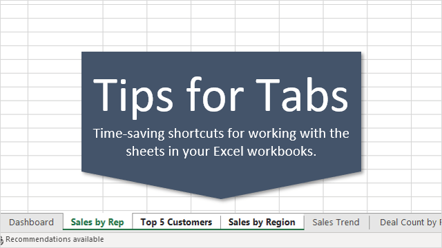
Tips for Navigating Worksheet Tabs
If you work with Excel files that contain a lot of sheets, then you know how time consuming it can be to work with the tabs. So in this post I share a few quick tips and shortcuts to save time with navigating your workbook.
#1 Copy Worksheets with Ctrl+Drag
This is one of my favorite shortcuts that every Excel user should know. The quickest way to make a duplicate copy of a sheet is using the Ctrl+Drag method. Here are the steps.
- Left-click and hold on the sheet you want to copy.
- Press and hold the Ctrl key. A plus symbol will appear in the sheet mouse icon.
- Drag the sheet to the right until the down arrow appears to the right of the sheet.
- Release the left mouse button. Then release the Ctrl key.
I broke it out into 4 steps, but it really feels like 2 steps once you get the hang of it. It’s much faster than right-clicking the tab and going to the Move or Copy… menu.
You can also use this technique when multiple sheets are selected. More on that below.
If you are in need of a high-five or pat on the back (and who isn’t), then feel free to share this one with your boss and co-workers. 🙂
#2 Navigating to the First or Last Sheet
If your workbook has a lot of tabs then you might want to quickly navigate to the first or last sheet in the workbook.
In Excel 2010 and earlier this was easy. There were dedicated buttons to scroll to the first or last sheet in the workbook.
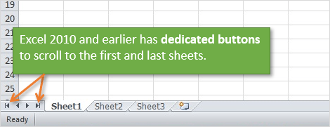
Starting in Excel 2013 we lost the dedicated buttons to navigate to the first or last sheet. These actions were consolidated into the sheet navigation buttons in the bottom left corner of the application window.
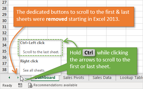
You now have to hold the Ctrl key when clicking the sheet navigation buttons to scroll to the first or last sheet. You can see this tip by hovering your mouse over the buttons.
So yes, this action now requires two hands unless you have really really long fingers or use a left-handed mouse. Something to brag about lefties… 😉
Once you have scrolled to the front/back, you can then click the first/last sheet to select it.
If you want to speed up this process, checkout my post on how to Create Keyboard Shortcuts to Select the First or Last Sheet in Excel. This is much faster than scrolling, then selecting the first/last sheet with the mouse.
#3 Select Next or Previous Sheet
If you’re a keyboard shortcut lover, like me, here are a few shortcuts to quickly move between sheets.
The keyboard shortcut to select the next sheet is: Ctrl+Page Down
The keyboard shortcut to select the previous sheet is: Ctrl+Page Up
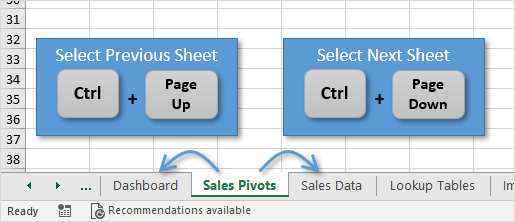
These are great if you are toggling back and forth between two sheets. Just move the sheets next to each other. You can then copy/paste or audit the sheets without having to navigate all over the workbook.
Having the right keyboard can be important for us Excel users. Especially when you are using a laptop keyboard. Checkout my post on Best Keyboards for Excel Keyboard Shortcuts to learn more.
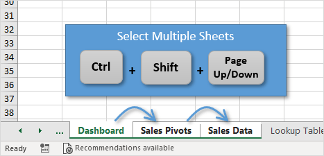
#4 Select Multiple Sheets
We can use the Ctrl and Shift keys to select multiple sheets.
Hold the Ctrl key and left-click sheet tabs to add them to the group of select sheets.
You can also hold the Shift key and left-click a sheet to select all sheets from the active sheet to the sheet you clicked.
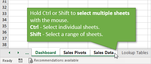
The keyboard shortcuts to select multiple sheets are Ctrl+Shift+Page Up / Page Down. This will select the previous/next sheet. You can continue to press this shortcut to select multiple sheets.
IMPORTANT NOTE About Selecting Multiple Sheets
When multiple sheets are selected, any changes you make the active sheet will also be applied to ALL selected sheets. This is a great time saver if you want to modify the value, formula, or formatting of specific cells on multiple sheets at the same time.
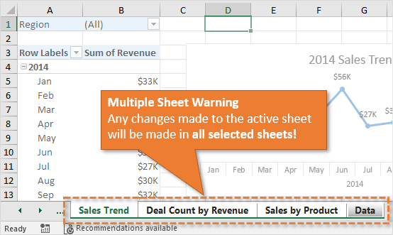
However, if you forget to ungroup the sheets (see tip #6) then you could really mess up your workbook. I’ve done this more times than I’d like to admit.
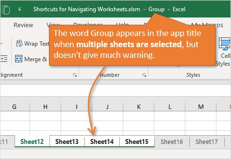
When you have multiple sheets selected, the word “Group” appears after the file name in the header of the Excel application window. This is not much of a warning though. I wish the application would turn a different color, or do a better job of warning us.
If you make a lot of edits to a sheet without realizing multiple sheets are selected it can spell disaster. Sometimes you won’t be able to undo the changes, and then have to pray that you saved the file.
#5 Select All Sheets
To select all sheets in the workbook, right-click any tab and choose Select All Sheets.
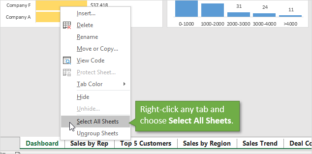
The same rule applies here. Any edits you make to the active sheet will also be made on all of the other selected sheets.
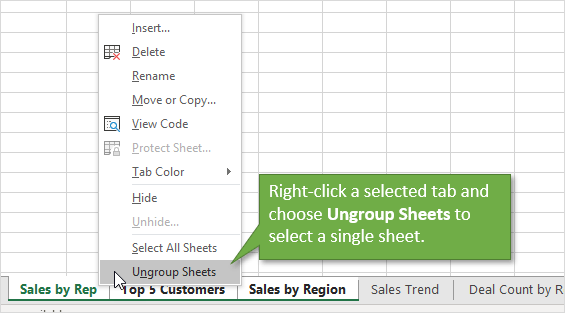
#6 Deselect (Ungroup) Sheets
To deselect multiple sheets you can just click on any tab that is not in the current selection.
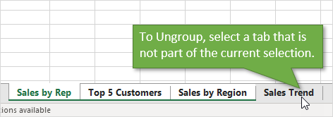
You can also right-click any of the selected tabs and choose Ungroup Sheets. The tab that you right-click will become the active sheet.
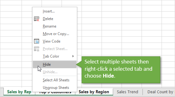
#7 Hide & Unhide Multiple Sheets
To hide multiple sheets:
- Select the sheets using the methods mentioned above.
- Right-click one of the selected tabs.
- Choose Hide.
The sheets will be hidden.
Unfortunately, unhiding multiple sheets is not directly possible in Excel. When you right-click a tab and choose Unhide, you can only select one sheet from the list of hidden sheets in the Unhide window.
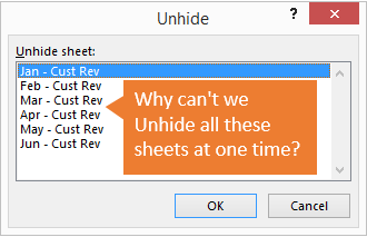
I have a post on 3 Ways to Unhide Multiple Sheets in Excel that explains techniques for unhiding sheets with a macro.
Bonus Tip: Sheet List
If your workbook contains a lot of sheets then you can right-click the tab navigation buttons to see a list of all visible sheets. You can then double-click a sheet in the list to jump to it.
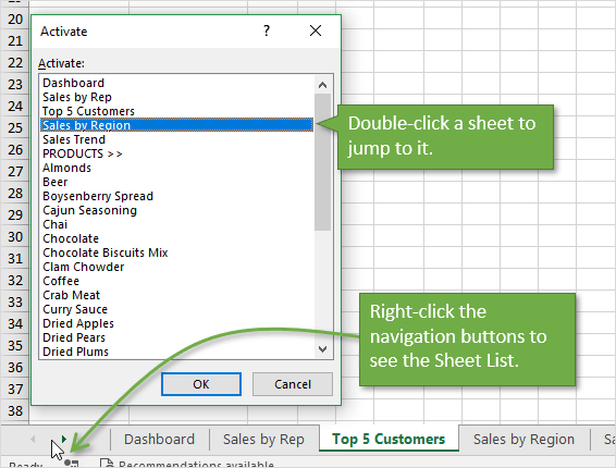
This list only shows the visible sheets in the workbook, and there is no way to search it.
So, I developed The Tab Hound Add-in to solve both of these problems and a lot more.
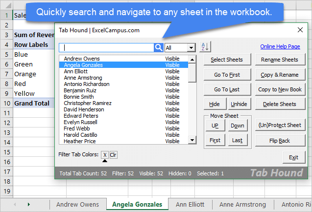
The add-in is packed with features (including unhiding multiple sheets) that make it faster & easier to navigate and modify the sheets in your workbooks.
I developed Tab Hound with VBA and the tools that are built into Excel. If you’d like to learn more about macros & VBA then checkout my free training webinar that is going on right now.

Click here to learn more and register for the webinar
Conclusion
I hope those tips help save some time out of your day. What are your favorite shortcuts for working with sheet tabs? Please leave a comment below with your suggestions, or any questions.
Thank you! 🙂
How to View List of Worksheet Tabs in Excel & Google Sheets — Aut…
Details:
https://www.datanumen.com/blogs/3-quick-ways-to
WebMethod 1: Get List Manually First off, open the specific Excel workbook. Then, double click on a sheet’s name in sheet list at the bottom. Next, press “Ctrl + C” to copy the name. Later, create a text file. Then, press “Ctrl + V” to paste the sheet name. … excel make tabs from list
› Verified Just Now
› Url: Automateexcel.com View Details
› Get more: Excel make tabs from listDetail Excel
How to View List of Worksheet Tabs in Excel & Google …
Details: WebTo see the whole list of worksheets, right-click the arrow to the left of the sheet tabs. All worksheet names are displayed in the pop-up list. To jump to a certain sheet, select the … formula for tab name in excel
› Verified 2 days ago
› Url: Automateexcel.com View Details
› Get more: Formula for tab name in excelDetail Excel
List sheet names with formula — Excel formula Exceljet
Details: WebTo list worksheets in an Excel workbook, you can use a 2-step approach: (1) define a named range called «sheetnames» with an old macro command and (2) use the INDEX … excel list of worksheets in workbook
› Verified 9 days ago
› Url: Exceljet.net View Details
› Get more: Excel list of worksheets in workbookDetail Excel
How To Generate A List Of Sheet Names From A …
Details: WebGo to the Formulas tab. Press the Define Name button. Enter SheetNames into the name field. Enter the following formula into the Refers to field. =REPLACE … excel tab names
› Verified 3 days ago
› Url: Howtoexcel.org View Details
› Get more: Excel tab namesDetail Excel
How to create a list of all worksheet names from a …
Details: WebThe following two VBA codes can help you list all of the worksheet names in a new worksheet. Please do as this: 1. Hold down the ALT + F11 keys to open the Microsoft Visual Basic for Applications … search multiple tabs in excel
› Verified Just Now
› Url: Extendoffice.com View Details
› Get more: Search multiple tabs in excelDetail Excel
Create list of tabs in Excel — Microsoft Community
Details: WebYou can do this only with VBA code. There is no worksheet function to get sheet names. Sub ListSheetNames () Dim R As Range Dim WS As Worksheet Set R = ActiveCell For Each WS In … view tabs in excel
› Verified Just Now
› Url: Answers.microsoft.com View Details
› Get more: View tabs in excelDetail Excel
7 Shortcuts for Working with Worksheet Tabs in Excel
Details: WebIf your workbook contains a lot of sheets then you can right-click the tab navigation buttons to see a list of all visible sheets. You can then double-click a sheet in the list to jump to it. This list only shows the … excel spreadsheet tabs not showing
› Verified 8 days ago
› Url: Excelcampus.com View Details
› Get more: Excel spreadsheet tabs not showingDetail Excel
How to View All Sheets in Excel at Once (5 Easy Ways) — ExcelDemy
Details: Web5 Easy Ways to View All Sheets in Excel at Once 1. View Two Sheets of Same Workbook Side by Side 2. Side by Side Seeing Two Sheets of Different Excel …
› Verified 9 days ago
› Url: Exceldemy.com View Details
› Get more: ExcelDetail Excel
Make Excel tabs list in a worksheet — Office Watch
Details: WebMake Excel tabs list in a worksheet 8 March 2019 Make your own clickable list of workbook tabs in an Excel worksheet to workaround the small number of tabs that can fit in a single line. See Fit more tabs …
› Verified 6 days ago
› Url: Office-watch.com View Details
› Get more: ExcelDetail Excel
Formula to list all sheet tabs under one spreadsheet
Details: WebHOW TO ATTACH YOUR SAMPLE WORKBOOK: Unregistered Fast answers need clear examples. Post a small Excel sheet (not a picture) showing realistic & …
› Verified 1 days ago
› Url: Excelforum.com View Details
› Get more: ExcelDetail Excel
Excel: Right Click to Show a Vertical Worksheets List
Details: Web1. Right-click the controls to the left of the tabs. 2. You’ll see a vertical list displayed in an Activate dialog box. Here, all sheets in your workbook are shown in an easily accessed vertical list. 3. Click on whatever sheet you …
› Verified 1 days ago
› Url: Knowledgewave.com View Details
› Get more: ExcelDetail Excel
Excel View All Worksheet Tabs in Big Workbooks — YouTube
Details: WebExcel Navigate Worksheet Tabs in Big Workbooks — Quick & Easy Learn how to navigate from one worksheet tab to another with ease in Excel. This is a handy sol
› Verified 3 days ago
› Url: Youtube.com View Details
› Get more: LearnDetail Excel
Combine data from multiple sheets — Microsoft Support
Details: WebOn the Data tab, in the Data Tools group, click Consolidate. In the Function box, click the function that you want Excel to use to consolidate the data. In each source sheet, select …
› Verified 3 days ago
› Url: Support.microsoft.com View Details
› Get more: ExcelDetail Excel
Excel Formula to List All Sheet Tab Names and include Hyperlinks
Details: WebMake navigating Excel workbooks with lots of sheets easy with this clever formula that automatically updates as new sheets are added/moved/renamed. Download
› Verified 3 days ago
› Url: Youtube.com View Details
› Get more: ExcelDetail Excel
Select worksheets — Microsoft Support
Details: WebBy keyboard: First, press F6 to activate the sheet tabs. Next, use the left or right arrow keys to select the sheet you want, then you can use Ctrl+Space to select that sheet. Repeat …
› Verified 7 days ago
› Url: Support.microsoft.com View Details
› Get more: ExcelDetail Excel
Automatic worksheet/tabs list in Excel — Office Watch
Details: WebNow we’ll take the next step and make an automatic list of worksheets that will update as the workbook changes. Simple code to get an Excel sheet list. List …
› Verified 5 days ago
› Url: Office-watch.com View Details
› Get more: ExcelDetail Excel
The Excel Ribbon GoSkills
Details: WebThe Excel ribbon tabs. There are nine tabs on the Excel Ribbon: File, Home, Insert, Page Layout, Formulas, Data, Review, View, and Help. The Home tab is the default tab when …
› Verified 3 days ago
› Url: Goskills.com View Details
› Get more: ExcelDetail Excel
Select All Worksheet Tabs — Automate Excel
Details: WebThe long way to select all Worksheet Tabs: 1. Select the First Sheet in the Workbook 2. Hold down Shift Key 3. Select the last worksheet in the Workbook The quicker way to …
› Verified 2 days ago
› Url: Automateexcel.com View Details
› Get more: ExcelDetail Excel
How can I list all worksheet tab names in another workbook in Excel?
Details: WebRebecca Fish. 1. Loop through workbooks by name and then loop through each sheet, copy workbook name in column A and worksheet name in column B n a new …
› Verified 2 days ago
› Url: Stackoverflow.com View Details
› Get more: ExcelDetail Excel
In this post we’ll find out how to get a list of all the sheet names in the current workbook without using VBA.
This can be pretty handy if you have a large workbook with hundreds of sheets and you want to create a table of contents. This method uses the little known and often forgotten Excel 4 macro functions.
These functions aren’t like Excel’s other functions such as SUM, VLOOKUP, INDEX etc. These functions won’t work in a regular sheet, they only work in named functions and macro sheets. For this trick we’re going to use one of these in a named function.
In this example, I’ve created a workbook with a lot of sheets. There are 50 sheets in this example so I was lazy and didn’t rename them from the default names.
Now we will create our named function.
- Go to the Formulas tab.
- Press the Define Name button.
- Enter SheetNames into the name field.
- Enter the following formula into the Refers to field.
=REPLACE(GET.WORKBOOK(1),1,FIND("]",GET.WORKBOOK(1)),"") - Hit the OK button.
In a sheet within the workbook enter the numbers 1,2,3,etc… into column A starting at row 2 and then in cell B2 enter the following formula and copy and paste it down the column until you have a list of all your sheet names.
=INDEX(SheetNames,A2)As a bonus, we can also create a hyperlink so that if you click on the link it will take you to that sheet. This can be handy for navigating through a spreadsheet with lots of sheets. To do this add this formula into the column C.
= HYPERLINK ( "#'" & B2 & "'!A1", "Go To Sheet" )Note, to use this method you will need to save the file as a macro enabled workbook (.xls, .xlsm or .xlsb). Not too difficult and no VBA needed.
Video Tutorial
This video will show you two methods to list all the sheet names in a workbook.
- The first method uses a VBA procedure from this post.
- The second (skip to 3:15 in the video) uses the method in the above post.
About the Author
John is a Microsoft MVP and qualified actuary with over 15 years of experience. He has worked in a variety of industries, including insurance, ad tech, and most recently Power Platform consulting. He is a keen problem solver and has a passion for using technology to make businesses more efficient.
Here’s the ‘old-fashioned’ way to make a list of worksheet tab names. It’s old because the formula uses ” Get.Workbook() ” which is an Excel 4 macro function that’s now blocked in modern Excel for security reasons. See Excel 4 macros are now blocked and about time tooWe’re including this older method for the sake of completeness and for users of older Excel
for Windows. See Automatic worksheet/tabs list in Excel – for a better way
- The old-fashioned method
- Gotchas
- Save as a macro workbook
- Only Excel for Windows
- Hidden tabs included
- Make the list automatically update
- Making the list
- Adding a clickable link to each tab
- Putting it all together
We’ve already talked about fitting more tabs on the screen or making a manual list of tabs/worksheets. Now we’ll take the next step and make an automatic list of worksheets that will update as the workbook changes.
Making a list of worksheets is a thing you might expect to be easy but is almost ludicrously intricate. There’s no direct function to do it and the long0-standing method relies on a very old and officially obsolete Excel function (which has no modern equivalent for reasons passing understanding).
In this article we’ll explain some ways to make an automatic list of worksheets. At the end we’ll show the ‘old-fashioned’ method that won’t work in modern Excel.
The steps are straightforward, even if you don’t understand the functions and formulas involved. We’ll break it down so you can understand how the whole thing comes together.
The old-fashioned method
Here’s the ‘old-fashioned’ way to make a list of worksheet tab names. It’s old because the formula uses ” Get.Workbook() ” which is an Excel 4 macro function that’s now blocked in modern Excel for security reasons. See Excel 4 macros are now blocked and about time too
We’re including this older method for the sake of completeness and for users of older Excel.
The tricky bit is making the initial list of tab names. Create a Define Name with a function which grabs the list of worksheets and puts them into an array. Go to Formulas | Define Name | Define Name …

Name: a label for the Name. We’re using SheetList
Refers to: this is the magic bit. Copy this formula:
=REPLACE(GET.WORKBOOK(1),1,FIND("]",GET.WORKBOOK(1)),"")
Get.Workbook() is the essential part. It’s an old Excel function that’s still necessary and available but not part of the current Excel function list. You won’t find it in the Formulas tab but it works fine … with some conditions we’ll mention in a moment.
To test your new name type =SheetList into a cell. The worksheet names will fill the cells to the right.

Gotchas
Let’s stop a moment to mention some of the little gotchas about this tip. It’s widely quoted on the Internet having been tweaked and adapted over time by various Excel wizards.
Too often the setbacks of this approach aren’t mentioned. Those mostly arise because the formula uses an obsolete function that Microsoft hasn’t replaced in modern Excel releases.
Save as a macro workbook
Because Get.Workbook() is an old Excel 4.0 function it can’t be saved in a ‘macro-free’ .xlsx workbook. If you try, an error appears.

Instead save as a macro-enabled workbook .xlsm . That’s a problem in some situations where macro-enabled Office documents are restricted or outright blocked due to security/virus risks.
Only Excel for Windows
Obsolete functions like Get.Workbook only work in Excel for Windows.
Other Excel’s (Mac, Online and apps) will show nasty #NAME errors instead.
Hidden tabs included
Get.Workbook includes any hidden workbooks. Here, the array example has the ‘Hide me away’ tab listed but it’s not on the tab list at the bottom of the worksheet.

All you can easily do is temporarily unhide any hidden tabs, move them to the end of the tabs list then rehide them. At least they’re grouped together at the end of your tabs list.
Make the list automatically update
The formula, and the array list it makes, has a limitation. It’s only refreshed when Excel thinks it’s necessary, which isn’t good enough in this case. Changes to the tabs or names might not be quickly reflected in the array list.
To make the array update automatically needs an old Excel trick to force recalculations:
&T(NOW())
NOW() returns the current time and is automatically updated by Excel whenever it recalculates the worksheet. T() is a test for a text value with the useful property of returning an empty string ( “” ) if the function contents are NOT text. NOW() always returns a date/time (obviously) so &T(NOW()) will always add nothing to a string. Because the name formula has the NOW() function, Excel will recalculate the entire name whenever a recalc occurs. In Excel parlance NOW() is a volatile function which makes the whole name formula volatile.
Go back to Formulas | Name Manager and change the SheetList name formula. Add &T(NOW()) at the end.
=REPLACE(GET.WORKBOOK(1),1,FIND("]",GET.WORKBOOK(1)),"") &T(NOW())
Making the list
Now we have an array list of the tabs you have many choices for presenting that list in a worksheet.
Start by putting this formula into the A2 cell
=INDEX(SheetList,ROWS($A$2:$A2))
- We’re assuming row 1 is for headings. If not use $A$1:$A1
- if you need to start in another cell or column, change the $A$2:$A2 reference accordingly.

Then click and drag the first cell down the column to clone it into other cells. Stop when you’ve copied enough cells for the number of tabs.

If you’ve gone too far, #REF will appear. If there’s a chance that more worksheets will be added later, you might want to keep those error formulas in place.
Adding a clickable link to each tab
Make links in Excel with the Hyperlink() function.
Hyperlink(<link>,<text to display>)
The <link> can be to parts of the Excel workbook, another workbook, a standard web page link or many other things. We’re just interested in links to each tab/worksheet like this.

Add this formula into column B
=HYPERLINK("#'"&A2&"'!A1","Clickable "&A2)
- We’ve added the work ‘Clickable’ in the example to show that the visible cell text can be anything you like. To see just the tab names use =HYPERLINK(“#’”&A2&”‘!A1”,A2)
- Again, change the cell reference as necessary.
Drag and copy the cell down, just like in the first column.
Putting it all together
Most likely you won’t need a separate list of tabs and clickable versions. Just one list of the worksheets that’s also clickable like this.
Here’s the formula for making a clickable list direct from the SheetList array.
=HYPERLINK("#'"&INDEX(SheetList,ROWS($A$2:$A2))&"'!A1",INDEX(SheetList,ROWS($A$2:$A2)))
We’ve changed the references to a worksheet name from “A2” (another cell in the current worksheet) with a reference direct to an element the SheetList array “INDEX(SheetList,ROWS($A$2:$A2))”
Yet again, drag and copy the first cell down
The worksheet tabs in Excel are rectangular tabs visible on the bottom left of the Excel workbook. The “Activate” tab shows the active worksheet available to edit. By default, there can be three worksheet tabs opened. We can insert more tabs in the worksheet using the plus button provided at the end of the tabs. We can also rename or delete any of the worksheet tabs.
Worksheets are the platform for Excel software. In addition, these worksheets have separate tabs. Every Excel file must contain at least one worksheet in it. We have many more things with these worksheets tab in Excel.
We can find the worksheet tab at the bottom of every Excel worksheet tab.
In this article, we will take a complete tour of worksheet tabs regarding how to manage worksheets, rename, delete, hide, unhide, move or copy, the replica of the current worksheet, and many other things.
Table of contents
- Worksheet Tab in Excel
- #1 Change No. of Worksheets by Default Excel Creates
- #2 Create Replica of Current Worksheet
- #3 – Create Replica of Current Worksheet by Using Shortcut Key
- #4 – Create New Excel Worksheet
- #5 – Create New Excel Worksheet Tab Using Shortcut Key
- #6 – Go to the First Worksheet & Last Worksheet
- #7 – Move Between Worksheets
- #8 – Delete Worksheets
- #9 – View All the Worksheets
- Things to Remember
- Recommended Articles
You are free to use this image on your website, templates, etc, Please provide us with an attribution linkArticle Link to be Hyperlinked
For eg:
Source: Excel Worksheet Tab (wallstreetmojo.com)
#1 Change No. of Worksheets by Default Excel Creates
You may have observed while opening the Excel file that it gives you three worksheets named “Sheet1,” “Sheet2,” and “Sheet3.”
We can modify this default setting and make our settings. Follow the below steps to change the settings.
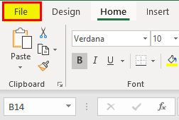
- We must first go to the “FILE.”

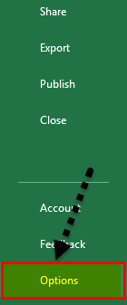
- Then, go to “OPTIONS.”

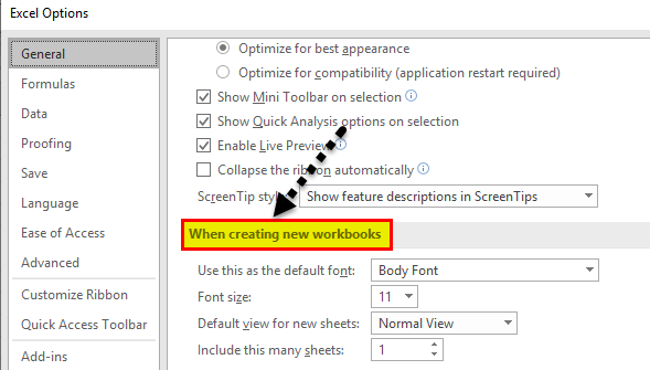
- Under “GENERAL,” go-to “When creating new workbooks.”

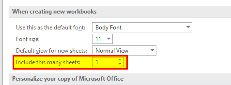
- Under this, we must choose “Include this many sheets.”

- Here, we can modify how many worksheets tab in Excel must be included while creating a new workbook.

- Click on “OK.” We will have a 5 Excel worksheets tab whenever we open a new workbook.


#2 Create Replica of Current Worksheet
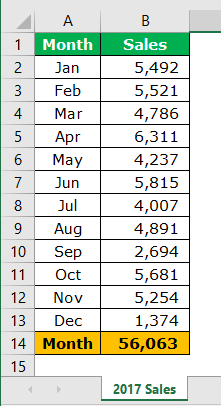
When you are working on an Excel file, you want to have a copy of the current worksheet at a certain point. For example, assume below is the worksheet tab you are working on at the moment.
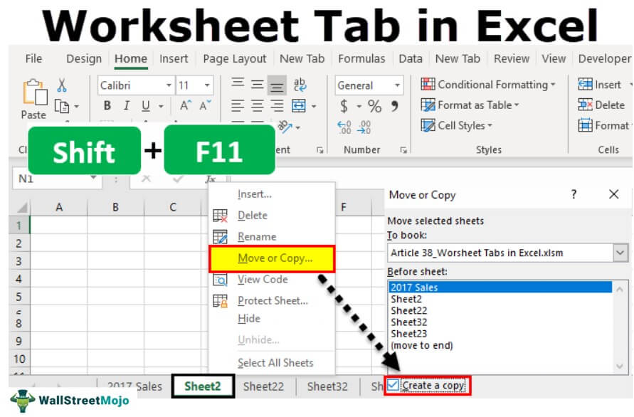
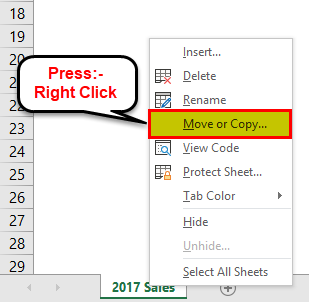
- Step 1: First, we must right-click on the worksheet and select “Move or Copy.”
- Step 2: In the below window, click the checkbox “Create a copy.”
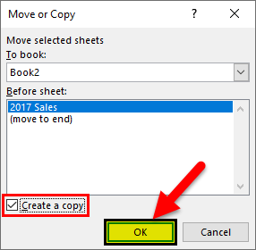
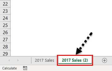
- Step 3: Click on “OK.” We will have a new sheet with the same data. The new worksheet name will be “2017 Sales (2).“
#3 – Create Replica of Current Worksheet by Using Shortcut Key
We can also create a replica of the current sheet by using this shortcut key.
- Step 1: We must select the sheet and hold the “Ctrl” key.
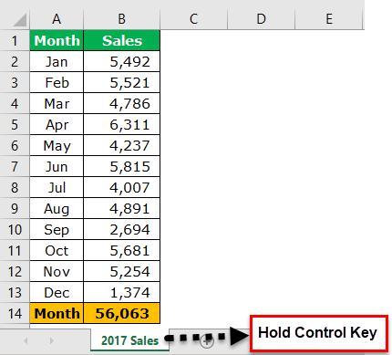
- Step 2: After holding the “Ctrl” key, hold the left button of the mouse key, and drag it to the right side. As a result, we would have a replica sheet now.
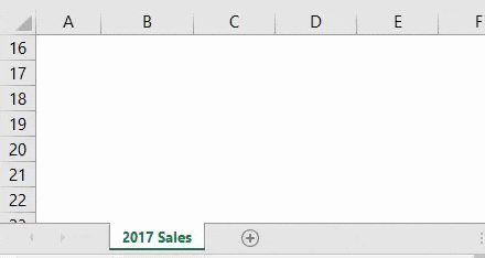
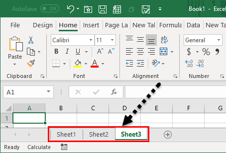
#4 – Create New Excel Worksheet
- Step 1: To create a new worksheet, we must click on the “plus” icon after the last worksheet.
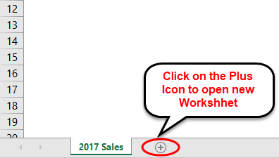
- Step 2: Once we click on the “PLUS” icon, we will have a new worksheet to the right of the current worksheet.

#5 – Create New Excel Worksheet Tab Using Shortcut Key
We can also create a new Excel worksheet tab using the shortcut key. For example, the shortcut key to insert the worksheet is “Shift + F11.”
If we press this key, it will insert the new worksheet tab to the left of the current worksheet.
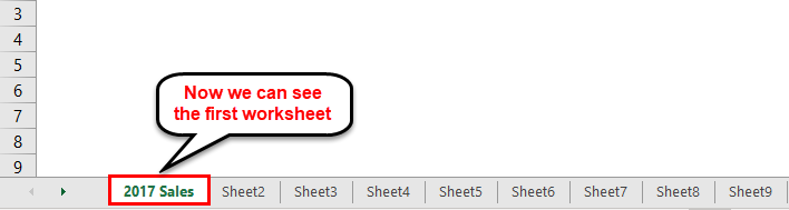
#6 – Go to the First Worksheet & Last Worksheet
Assume we are working with the workbook, which has many worksheets. Furthermore, we are moving between sheets regularly. Therefore, if we want to move to the last and first worksheets, we need to use the below technique.
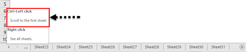
To come to the first worksheet, we must hold the “Ctrl” key and click on the arrow symbol to move to the first sheet.
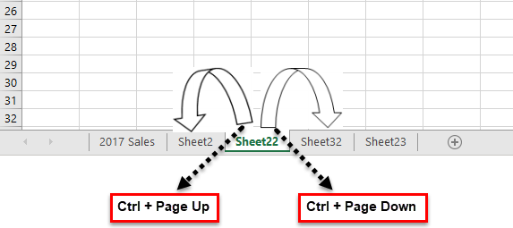
#7 – Move Between Worksheets
Going through all the worksheets in the workbook is a tough task if we move manually. So, we have shortcut keys to move between worksheets.
Ctrl + Page Up: This would go to the previous worksheet.
Ctrl + Page Down: This would go to the next worksheet.
#8 – Delete Worksheets
Like how we can insert new worksheets, we can delete the worksheet. To delete the worksheet, we must right-click on the required worksheet and click on “DELETE”.
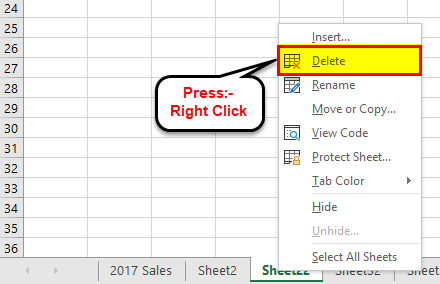
If you want to delete multiple sheets simultaneously, we must hold the “Ctrl” key and select the sheets we want to delete.
Now, we can delete all the sheets at once.
We can also delete the sheet using the shortcut key, “ALT + E + L.”

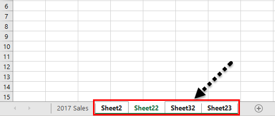
If we want to select all the sheets, we can right-click on any worksheets and choose “Select All Sheets.”
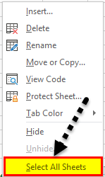
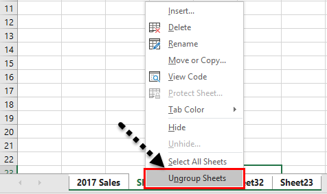
Once all the worksheets are selected, and if we want to unselect again, we must right-click on any worksheets and choose “Ungroup Worksheets.”
#9 – View All the Worksheets
If we have many worksheets and want to select a particular sheet, we do not know where exactly that sheet is.
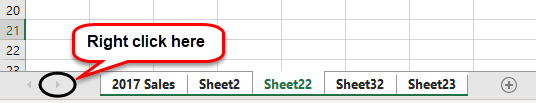
We can use the below technique to see all the worksheets. But, first, we must right-click on the move buttons at the bottom.
Consequently, we would see below the list of all the worksheets tab in the Excel file.
Things to Remember
- We can also hide and unhide sheets by right click on the sheetsThere are different methods to Unhide Sheets in Excel as per the need to unhide all, all except one, multiple, or a particular worksheet. You can use Right Click, Excel Shortcut Key, or write a VBA code in Excel. read more.
- The shortcut key is “ALT + E + L.”
- For creating a replica sheet, the shortcut key is “ALT + E + M.”
- The shortcut key to select left side worksheets is “Ctrl + Page Up.”
- The shortcut key to select right side worksheets is “Ctrl + Page Down.”
Recommended Articles
This article has been guided to the Worksheet Tab in Excel. Here, we discuss how to manage worksheets, rename, delete, hide, unhide, move or copy and use shortcut keys with practical examples and a downloadable Excel template. You may learn more about Excel from the following articles: –
- Insert Tab in Excel
- What is Accounting Worksheet?
- Excel VBA Worksheets
- Strikethrough in Excel