
Содержание
- Create or delete a custom list for sorting and filling data
- Need more help?
- Analyze and format
- Create and format tables
- Try it!
- How to control and understand settings in the Format Cells dialog box in Excel
- Summary
- More Information
- Number Tab
- Auto Number Formatting
- Built-in Number Formats
- Custom Number Formats
Create or delete a custom list for sorting and filling data
Use a custom list to sort or fill in a user-defined order. Excel provides day-of-the-week and month-of-the year built-in lists, but you can also create your own custom list.
To understand custom lists, it is helpful to see how they work and how they are stored on a computer.
Comparing built-in and custom lists
Excel provides the following built-in, day-of-the-week, and month-of-the year custom lists.
Sun, Mon, Tue, Wed, Thu, Fri, Sat
Sunday, Monday, Tuesday, Wednesday, Thursday, Friday, Saturday
Jan, Feb, Mar, Apr, May, Jun, Jul, Aug, Sep, Oct, Nov, Dec
January, February, March, April, May, June, July, August, September, October, November, December
Note: You cannot edit or delete a built-in list.
You can also create your own custom list, and use them to sort or fill. For example, if you want to sort or fill by the following lists, you’ll need to create a custom list, since there is no natural order.
High, Medium, Low
Large, Medium, and Small
North, South, East, and West
Senior Sales Manager, Regional Sales Manager, Department Sales Manager, and Sales Representative
A custom list can correspond to a cell range, or you can enter the list in the Custom Lists dialog box.
Note: A custom list can only contain text or text that is mixed with numbers. For a custom list that contains numbers only, such as 0 through 100, you must first create a list of numbers that is formatted as text.
There are two ways to create a custom list. If your custom list is short, you can enter the values directly in the popup window. If your custom list is long, you can import it from a range of cells.
Enter values directly
Follow these steps to create a custom list by entering values:
For Excel 2010 and later, click File > Options > Advanced > General > Edit Custom Lists.
For Excel 2007, click the Microsoft Office Button  > Excel Options > Popular > Top options for working with Excel > Edit Custom Lists.
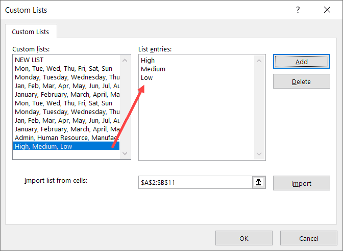
In the Custom Lists box, click NEW LIST, and then type the entries in the List entries box, beginning with the first entry.
Press the Enter key after each entry.
When the list is complete, click Add.
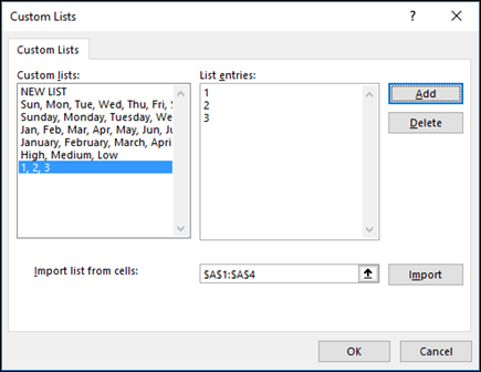
The items in the list that you have chosen will appear in the Custom lists panel.
Create a custom list from a cell range
Follow these steps:
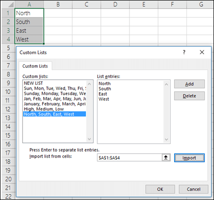
In a range of cells, enter the values that you want to sort or fill by, in the order that you want them, from top to bottom. Select the range of cells you just entered, and follow the previous instructions for displaying the Edit Custom Lists popup window.
In the Custom Lists popup window, verify that the cell reference of the list of items that you have chosen appears in the Import list from cells field, and then click Import.
The items in the list that you have chosen will appear in the Custom Lists panel.
 Options > Advanced > General > Edit Custom Lists. For Excel 2007 click the Office Button > Excel Options > Popular > Edit Custom Lists.» loading=»lazy»>
Note: You can only create a custom list according to values, such as text, numbers, dates or times. You cannot create a custom list for formats such as cell color, font color, or an icon.
Follow these steps:
Follow the previous instructions for displaying the Edit Custom Lists dialog.
In the Custom Lists box, choose the list that you want to delete, and then click Delete.
Once you create a custom list, it is added to your computer registry, so that it is available for use in other workbooks. If you use a custom list when sorting data, it is also saved with the workbook, so that it can be used on other computers, including servers where your workbook might be published to Excel Services and you want to rely on the custom list for a sort.
However, if you open the workbook on another computer or server, you do not see the custom list that is stored in the workbook file in the Custom Lists popup window that is available from Excel Options, only from the Order column of the Sort dialog box. The custom list that is stored in the workbook file is also not immediately available for the Fill command.
If you prefer, add the custom list that is stored in the workbook file to the registry of the other computer or server and make it available from the Custom Lists popup window in Excel Options. From the Sort popup window, in the Order column, select Custom Lists to display the Custom Lists popup window, then select the custom list, and then click Add.
Need more help?
You can always ask an expert in the Excel Tech Community or get support in the Answers community.
Источник
Analyze and format
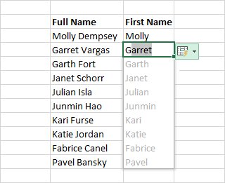
Automatically fill a column with Flash Fill
For example, automatically fill a First Name column from a Full Name column.
In the cell under First Name, type Molly and press Enter.
In the next cell, type the first few letters of Garret.
When the list of suggested values appears, press Return.
Select Flash Fill Options  for more options.
Try it! Select File > New, select Take a tour, and then select the Fill Tab.
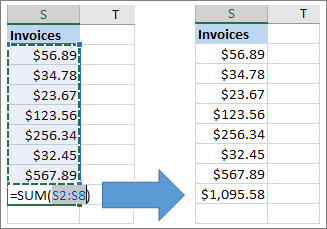
Quickly calculate with AutoSum
Select the cell below the numbers you want to add.
Select Home > AutoSum  .
.
Tip For more calculations, select the down arrow next to AutoSum, and select a calculation.
You can also select a range of numbers to see common calculations in the status bar. See View summary data on the status bar.
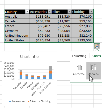
Use the Quick Analysis tool to pick the right chart for your data.
Select the data you want to show in a chart.
Select the Quick Analysis button  to the bottom-right of the selected cells.
Select Charts, hover over the options, and pick the chart you want.
Try it! Select File > New, select Take a tour, and then select the Charts tab. For more information, see Create charts.
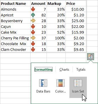
Use conditional formatting
Use Quick Analysis to highlight important data or show data trends.
Select the data to conditionally format.
Select the Quick Analysis button to the bottom-right of the selected cells.
Select Formatting, hover over the options, and pick the one you want.
Try it! Select File > New, select Take a tour, and then select the Analyze Tab.
Freeze the top row of headings
Freeze the top row of column headings so that only the data scrolls.
Press Enter or Esc to make sure you’re done editing a cell.
Select View > Freeze Panes > Freeze Top Row.
Источник
Create and format tables
Create and format a table to visually group and analyze data.
Note: Excel tables shouldn’t be confused with the data tables that are part of a suite of What-If Analysis commands ( Forecast, on the Data tab). See Introduction to What-If Analysis for more information.

Try it!
Select a cell within your data.
Select Home > Format as Table.
Choose a style for your table.
In the Create Table dialog box, set your cell range.
Mark if your table has headers.
Insert a table in your spreadsheet. See Overview of Excel tables for more information.
Select a cell within your data.
Select Home > Format as Table.
Choose a style for your table.
In the Create Table dialog box, set your cell range.
Mark if your table has headers.
To add a blank table, select the cells you want included in the table and click Insert > Table.
To format existing data as a table by using the default table style, do this:
Select the cells containing the data.
Click Home > Table > Format as Table.
If you don’t check the My table has headers box, Excel for the web adds headers with default names like Column1 and Column2 above the data. To rename a default header, double-click it and type a new name.
Note: You can’t change the default table formatting in Excel for the web.
Источник
How to control and understand settings in the Format Cells dialog box in Excel
Summary
Microsoft Excel lets you change many of the ways it displays data in a cell. For example, you can specify the number of digits to the right of a decimal point, or you can add a pattern and border to the cell. You can access and modify the majority of these settings in the Format Cells dialog box (on the Format menu, click Cells).
The «More Information» section of this article provides information about each of the settings available in the Format Cells dialog box and how each of these settings can affect the way your data is presented.
More Information
There are six tabs in the Format Cells dialog box: Number, Alignment, Font, Border, Patterns, and Protection. The following sections describe the settings available in each tab.
Number Tab
Auto Number Formatting
By default, all worksheet cells are formatted with the General number format. With the General format, anything you type into the cell is usually left as-is. For example, if you type 36526 into a cell and then press ENTER, the cell contents are displayed as 36526. This is because the cell remains in the General number format. However, if you first format the cell as a date (for example, d/d/yyyy) and then type the number 36526, the cell displays 1/1/2000.
There are also other situations where Excel leaves the number format as General, but the cell contents are not displayed exactly as they were typed. For example, if you have a narrow column and you type a long string of digits like 123456789, the cell might instead display something like 1.2E+08. If you check the number format in this situation, it remains as General.
Finally, there are scenarios where Excel may automatically change the number format from General to something else, based on the characters that you typed into the cell. This feature saves you from having to manually make the easily recognized number format changes. The following table outlines a few examples where this can occur:
| If you type | Excel automatically assigns this number format |
|---|---|
| 1.0 | General |
| 1.123 | General |
| 1.1% | 0.00% |
| 1.1E+2 | 0.00E+00 |
| 1 1/2 | # ?/? |
| $1.11 | Currency, 2 decimal places |
| 1/1/01 | Date |
| 1:10 | Time |
Generally speaking, Excel applies automatic number formatting whenever you type the following types of data into a cell:
Built-in Number Formats
Excel has a large array of built-in number formats from which you can choose. To use one of these formats, click any one of the categories below General and then select the option that you want for that format. When you select a format from the list, Excel automatically displays an example of the output in the Sample box on the Number tab. For example, if you type 1.23 in the cell and you select Number in the category list, with three decimal places, the number 1.230 is displayed in the cell.
These built-in number formats actually use a predefined combination of the symbols listed below in the «Custom Number Formats» section. However, the underlying custom number format is transparent to you.
The following table lists all of the available built-in number formats:
| Number format | Notes |
|---|---|
| Number | Options include: the number of decimal places, whether or not the thousands separator is used, and the format to be used for negative numbers. |
| Currency | Options include: the number of decimal places, the symbol used for the currency, and the format to be used for negative numbers. This format is used for general monetary values. |
| Accounting | Options include: the number of decimal places, and the symbol used for the currency. This format lines up the currency symbols and decimal points in a column of data. |
| Date | Select the style of the date from the Type list box. |
| Time | Select the style of the time from the Type list box. |
| Percentage | Multiplies the existing cell value by 100 and displays the result with a percent symbol. If you format the cell first and then type the number, only numbers between 0 and 1 are multiplied by 100. The only option is the number of decimal places. |
| Fraction | Select the style of the fraction from the Type list box. If you do not format the cell as a fraction before typing the value, you may have to type a zero or space before the fractional part. For example, if the cell is formatted as General and you type 1/4 in the cell, Excel treats this as a date. To type it as a fraction, type 0 1/4 in the cell. |
| Scientific | The only option is the number of decimal places. |
| Text | Cells formatted as text will treat anything typed into the cell as text, including numbers. |
| Special | Select one of the following from the Type box: Zip Code, Zip Code + 4, Phone Number, and Social Security Number. |
Custom Number Formats
If one of the built-in number formats does not display the data in the format that you require, you can create your own custom number format. You can create these custom number formats by modifying the built-in formats or by combining the formatting symbols into your own combination.
Before you create your own custom number format, you need to be aware of a few simple rules governing the syntax for number formats:
Each format that you create can have up to three sections for numbers and a fourth section for text.
The first section is the format for positive numbers, the second for negative numbers, and the third for zero values.
These sections are separated by semicolons.
If you have only one section, all numbers (positive, negative, and zero) are formatted with that format.
You can prevent any of the number types (positive, negative, zero) from being displayed by not typing symbols in the corresponding section. For example, the following number format prevents any negative or zero values from being displayed:
To set the color for any section in the custom format, type the name of the color in brackets in the section. For example, the following number format formats positive numbers blue and negative numbers red:
Instead of the default positive, negative and zero sections in the format, you can specify custom criteria that must be met for each section. The conditional statements that you specify must be contained within brackets. For example, the following number format formats all numbers greater than 100 as green, all numbers less than or equal to -100 as yellow, and all other numbers as cyan:
Источник
Содержание
- Форматирование таблиц
- Автоформатирование
- Переход к форматированию
- Форматирование данных
- Выравнивание
- Шрифт
- Граница
- Заливка
- Защита
- Вопросы и ответы

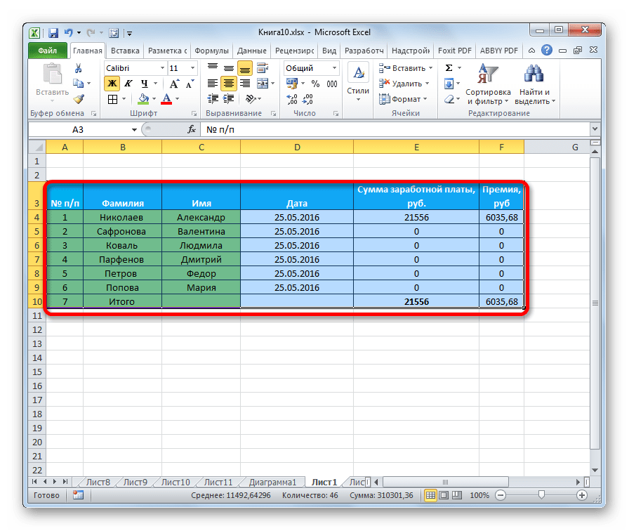
Одним из самых важных процессов при работе в программе Excel является форматирование. С его помощью не только оформляется внешний вид таблицы, но и задается указание того, как программе воспринимать данные, расположенные в конкретной ячейке или диапазоне. Без понимания принципов работы данного инструмента нельзя хорошо освоить эту программу. Давайте подробно выясним, что же представляет собой форматирование в Экселе и как им следует пользоваться.
Урок: Как форматировать таблицы в Microsoft Word
Форматирование таблиц
Форматирование – это целый комплекс мер регулировки визуального содержимого таблиц и расчетных данных. В данную область входит изменение огромного количества параметров: размер, тип и цвет шрифта, величина ячеек, заливка, границы, формат данных, выравнивание и много другое. Подробнее об этих свойствах мы поговорим ниже.
Автоформатирование
К любому диапазону листа с данными можно применить автоматическое форматирование. Программа отформатирует указанную область как таблицу и присвоит ему ряд предустановленных свойств.
- Выделяем диапазон ячеек или таблицу.
- Находясь во вкладке «Главная» кликаем по кнопке «Форматировать как таблицу». Данная кнопка размещена на ленте в блоке инструментов «Стили». После этого открывается большой список стилей с предустановленными свойствами, которые пользователь может выбрать на свое усмотрение. Достаточно просто кликнуть по подходящему варианту.
- Затем открывается небольшое окно, в котором нужно подтвердить правильность введенных координат диапазона. Если вы выявили, что они введены не верно, то тут же можно произвести изменения. Очень важно обратить внимание на параметр «Таблица с заголовками». Если в вашей таблице есть заголовки (а в подавляющем большинстве случаев так и есть), то напротив этого параметра должна стоять галочка. В обратном случае её нужно убрать. Когда все настройки завершены, жмем на кнопку «OK».
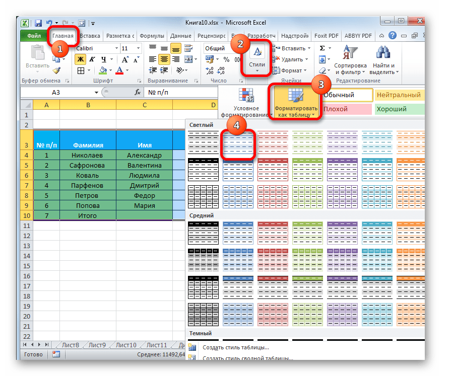

После этого, таблица будет иметь выбранный формат. Но его можно всегда отредактировать с помощью более точных инструментов форматирования.
Переход к форматированию
Пользователей не во всех случаях удовлетворяет тот набор характеристик, который представлен в автоформатировании. В этом случае, есть возможность отформатировать таблицу вручную с помощью специальных инструментов.
Перейти к форматированию таблиц, то есть, к изменению их внешнего вида, можно через контекстное меню или выполнив действия с помощью инструментов на ленте.
Для того, чтобы перейти к возможности форматирования через контекстное меню, нужно выполнить следующие действия.
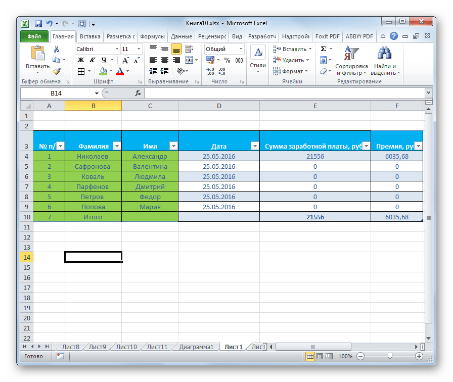
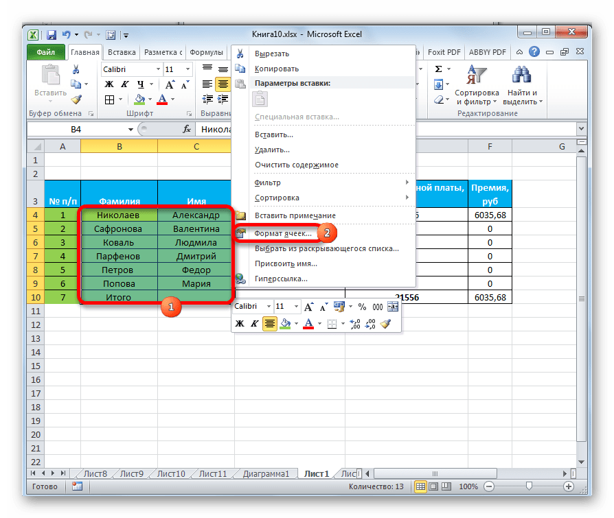
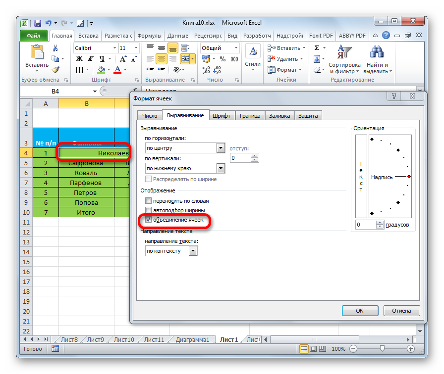
- Выделяем ячейку или диапазон таблицы, который хотим отформатировать. Кликаем по нему правой кнопкой мыши. Открывается контекстное меню. Выбираем в нем пункт «Формат ячеек…».
- После этого открывается окно формата ячеек, где можно производить различные виды форматирования.

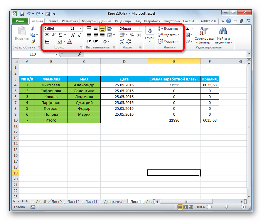
Инструменты форматирования на ленте находятся в различных вкладках, но больше всего их во вкладке «Главная». Для того, чтобы ими воспользоваться, нужно выделить соответствующий элемент на листе, а затем нажать на кнопку инструмента на ленте.
Форматирование данных
Одним из самых важных видов форматирования является формат типа данных. Это обусловлено тем, что он определяет не столько внешний вид отображаемой информации, сколько указывает программе, как её обрабатывать. Эксель совсем по разному производит обработку числовых, текстовых, денежных значений, форматов даты и времени. Отформатировать тип данных выделенного диапазона можно как через контекстное меню, так и с помощью инструмента на ленте.
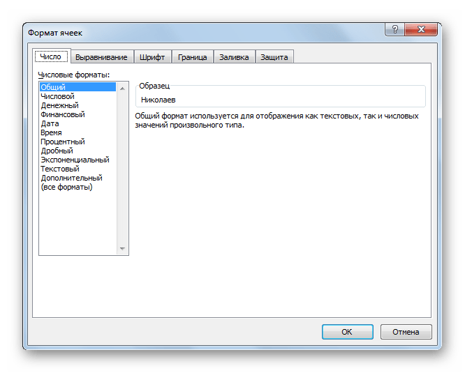
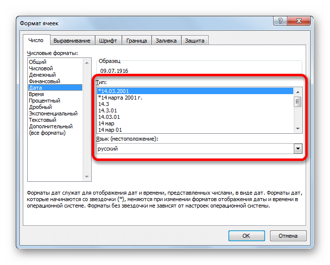
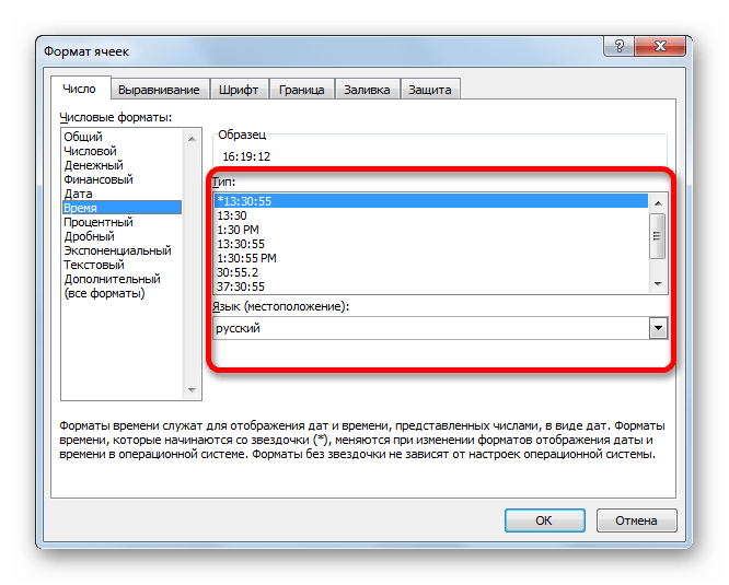
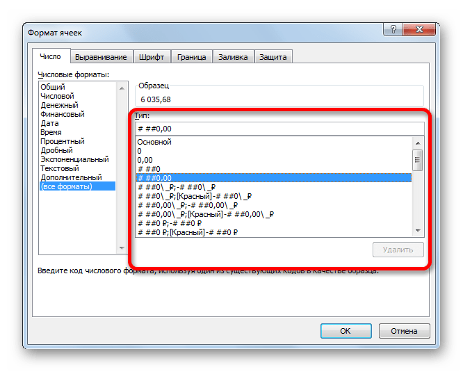
Если вы откроете окно «Формат ячеек» чрез контекстное меню, то нужные настройки будут располагаться во вкладке «Число» в блоке параметров «Числовые форматы». Собственно, это единственный блок в данной вкладке. Тут производится выбор одного из форматов данных:
- Числовой;
- Текстовый;
- Время;
- Дата;
- Денежный;
- Общий и т.д.
После того, как выбор произведен, нужно нажать на кнопку «OK».

Кроме того, для некоторых параметров доступны дополнительные настройки. Например, для числового формата в правой части окна можно установить, сколько знаков после запятой будет отображаться у дробных чисел и показывать ли разделитель между разрядами в числах.

Для параметра «Дата» доступна возможность установить, в каком виде дата будет выводиться на экран (только числами, числами и наименованиями месяцев и т.д.).
Аналогичные настройки имеются и у формата «Время».
Если выбрать пункт «Все форматы», то в одном списке будут показаны все доступные подтипы форматирования данных.
Если вы хотите отформатировать данные через ленту, то находясь во вкладке «Главная», нужно кликнуть по выпадающему списку, расположенному в блоке инструментов «Число». После этого раскрывается перечень основных форматов. Правда, он все-таки менее подробный, чем в ранее описанном варианте.
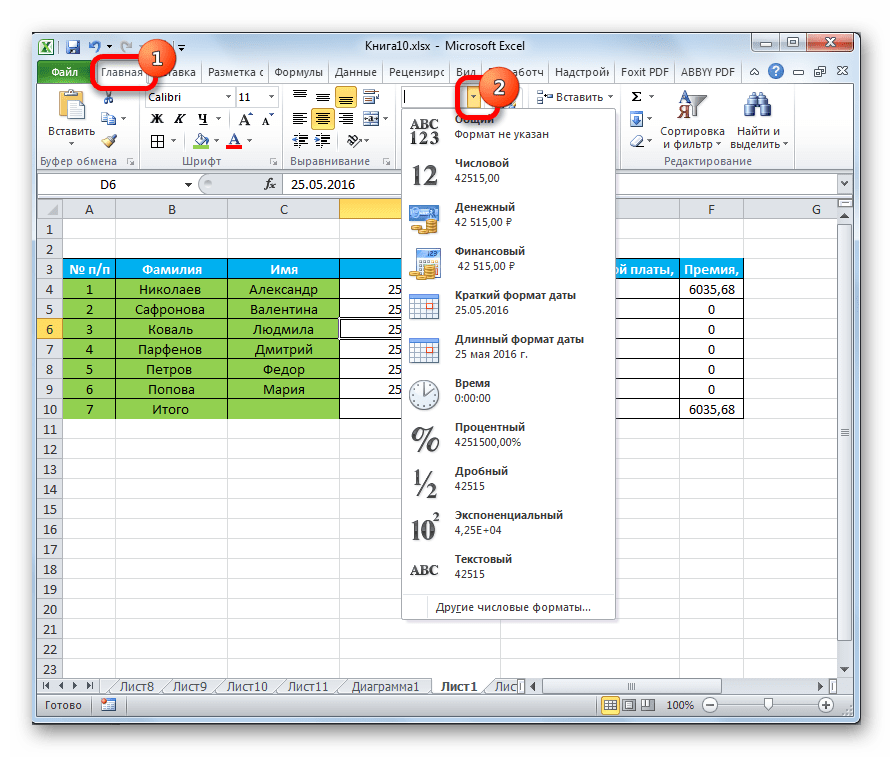
Впрочем, если вы хотите более точно произвести форматирование, то в этом списке нужно кликнуть по пункту «Другие числовые форматы…». Откроется уже знакомое нам окно «Формат ячеек» с полным перечнем изменения настроек.

Урок: Как изменить формат ячейки в Excel
Выравнивание
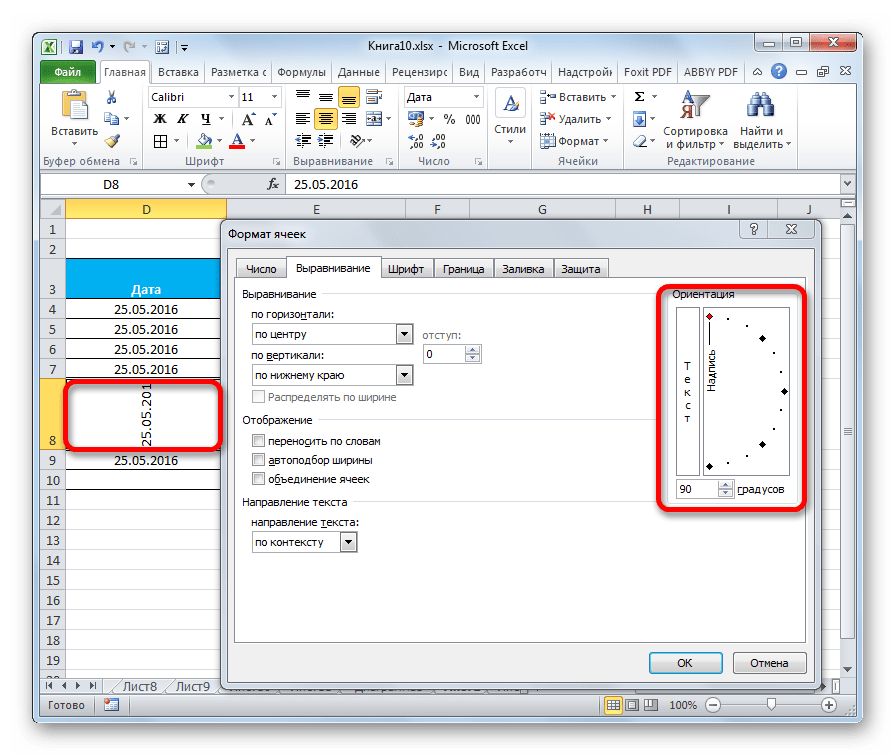
Целый блок инструментов представлен во вкладке «Выравнивание» в окне «Формат ячеек».
Путем установки птички около соответствующего параметра можно объединять выделенные ячейки, производить автоподбор ширины и переносить текст по словам, если он не вмещается в границы ячейки.
Кроме того, в этой же вкладке можно позиционировать текст внутри ячейки по горизонтали и вертикали.
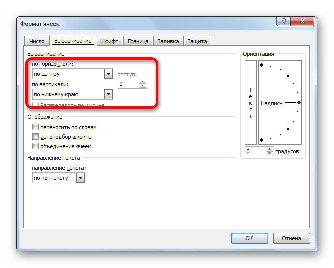
В параметре «Ориентация» производится настройка угла расположения текста в ячейке таблицы.
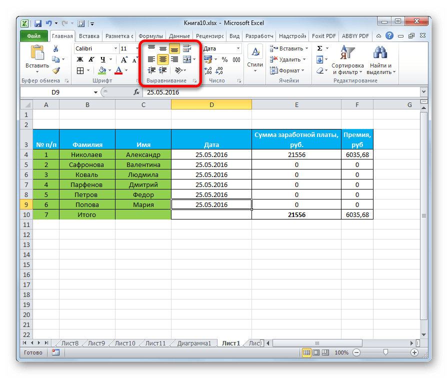
Блок инструментов «Выравнивание» имеется так же на ленте во вкладке «Главная». Там представлены все те же возможности, что и в окне «Формат ячеек», но в более усеченном варианте.
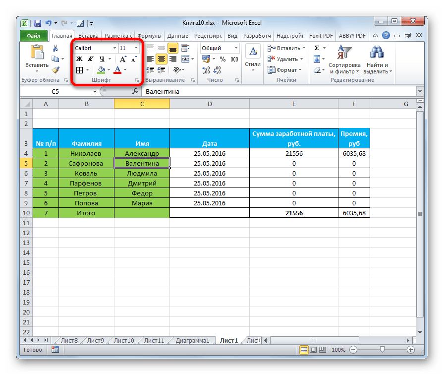
Шрифт
Во вкладке «Шрифт» окна форматирования имеются широкие возможности по настройке шрифта выделенного диапазона. К этим возможностям относятся изменение следующих параметров:
- тип шрифта;
- начертание (курсив, полужирный, обычный)
- размер;
- цвет;
- видоизменение (подстрочный, надстрочный, зачеркнутый).

На ленте тоже имеется блок инструментов с аналогичными возможностями, который также называется «Шрифт».
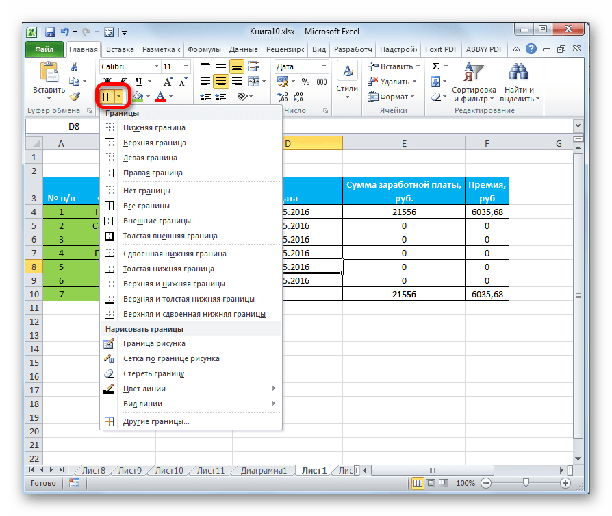
Граница
Во вкладке «Граница» окна форматирования можно настроить тип линии и её цвет. Тут же определяется, какой граница будет: внутренней или внешней. Можно вообще убрать границу, даже если она уже имеется в таблице.
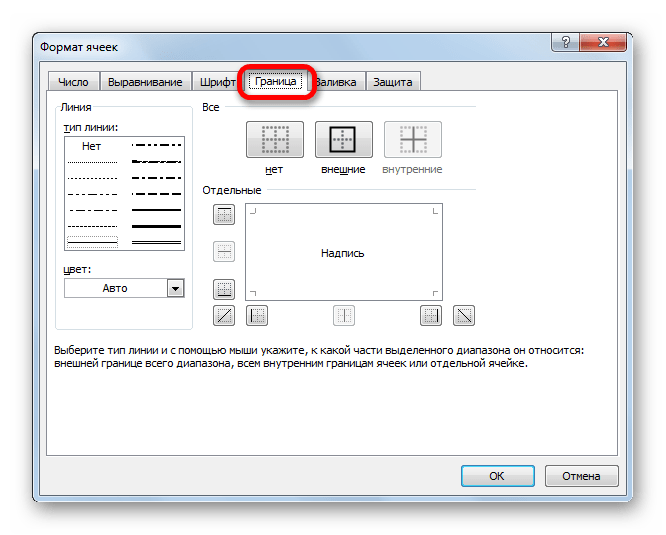
А вот на ленте нет отдельного блока инструментов для настроек границы. Для этих целей во вкладке «Главная» выделена только одна кнопка, которая располагается в группе инструментов «Шрифт».
Заливка
Во вкладке «Заливка» окна форматирования можно производить настройку цвета ячеек таблицы. Дополнительно можно устанавливать узоры.

На ленте, как и для предыдущей функции для заливки выделена всего одна кнопка. Она также размещается в блоке инструментов «Шрифт».
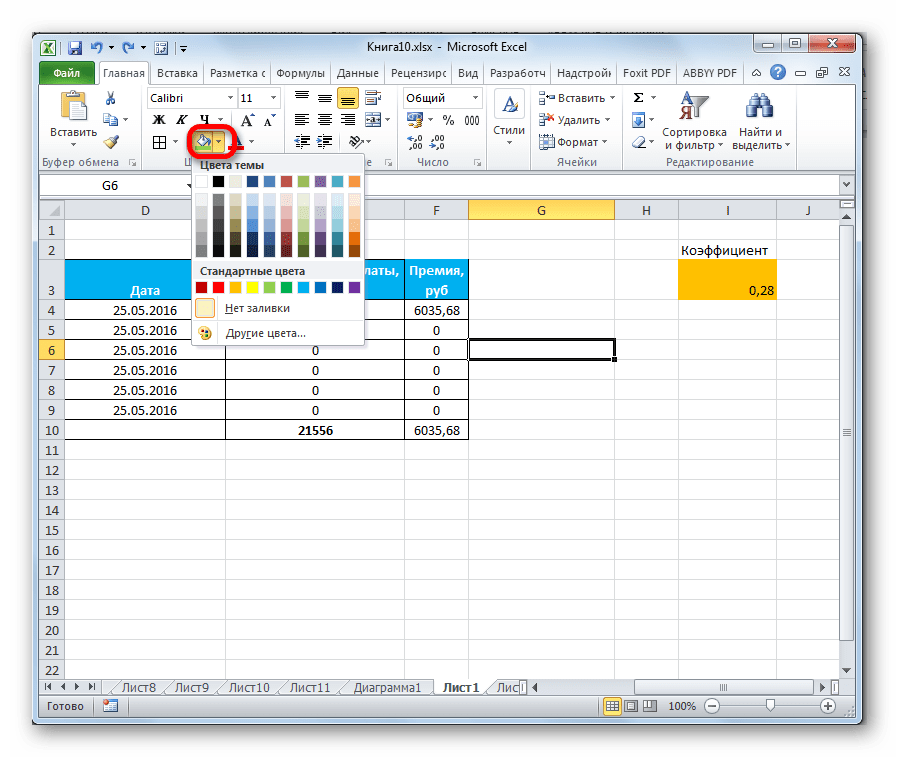
Если представленных стандартных цветов вам не хватает и вы хотите добавить оригинальности в окраску таблицы, тогда следует перейти по пункту «Другие цвета…».
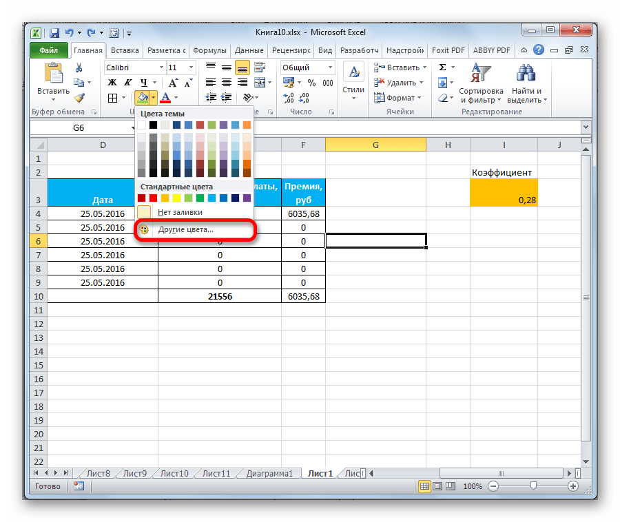
После этого открывается окно, предназначенное для более точного подбора цветов и оттенков.

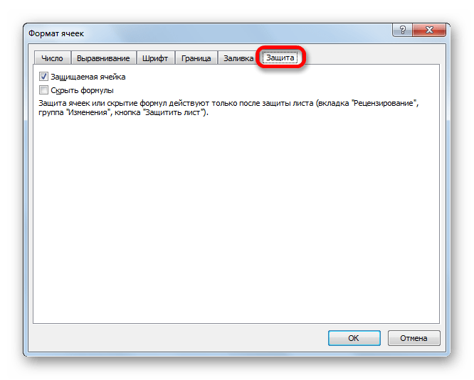
Защита
В Экселе даже защита относится к области форматирования. В окне «Формат ячеек» имеется вкладка с одноименным названием. В ней можно обозначить, будет ли защищаться от изменений выделенный диапазон или нет, в случае установки блокировки листа. Тут же можно включить скрытие формул.
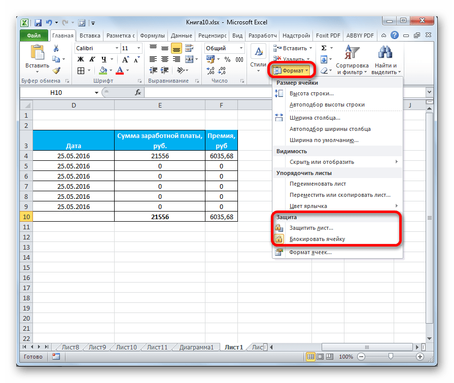
На ленте аналогичные функции можно увидеть после клика по кнопке «Формат», которая расположена во вкладке «Главная» в блоке инструментов «Ячейки». Как видим, появляется список, в котором имеется группа настроек «Защита». Причем тут можно не только настроить поведение ячейки в случае блокировки, как это было в окне форматирования, но и сразу заблокировать лист, кликнув по пункту «Защитить лист…». Так что это один из тех редких случаев, когда группа настроек форматирования на ленте имеет более обширный функционал, чем аналогичная вкладка в окне «Формат ячеек».
.
Урок: Как защитить ячейку от изменений в Excel
Как видим, программа Excel обладает очень широким функционалом по форматированию таблиц. При этом, можно воспользоваться несколькими вариантами стилей с предустановленными свойствами. Также можно произвести более точные настройки при помощи целого набора инструментов в окне «Формат ячеек» и на ленте. За редким исключением в окне форматирования представлены более широкие возможности изменения формата, чем на ленте.
Application examples of formatting Excel data of various types for computationally intensive calculations.
Changing of cells format in data tables
 Format Painter in Excel for table layout.
Multiple copies of table cell formats on multiple sheets using the Format Painter tool. Copying the width of columns and rows of a sheet.
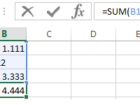 Influence of the cell format on working of the SUM function.
The possible errors in the summation, where there is a comma instead of a dot. Quick search of incorrect fractional numbers. Automatic assignment of the cell formats with the SUMM function.
 Transfer of data from one Excel table to another one.
You can transfer table data within one sheet, as well as to another sheet or to another file. In this case, you can copy either the entire table, or its individual values, properties or parameters.
Create or delete a custom list for sorting and filling data
Excel for Microsoft 365 Excel 2021 Excel 2019 Excel 2016 Excel 2013 Excel 2010 Excel 2007 More…Less
Use a custom list to sort or fill in a user-defined order. Excel provides day-of-the-week and month-of-the year built-in lists, but you can also create your own custom list.
To understand custom lists, it is helpful to see how they work and how they are stored on a computer.
Comparing built-in and custom lists
Excel provides the following built-in, day-of-the-week, and month-of-the year custom lists.
|
Built-in lists |
|
Sun, Mon, Tue, Wed, Thu, Fri, Sat |
|
Sunday, Monday, Tuesday, Wednesday, Thursday, Friday, Saturday |
|
Jan, Feb, Mar, Apr, May, Jun, Jul, Aug, Sep, Oct, Nov, Dec |
|
January, February, March, April, May, June, July, August, September, October, November, December |
Note: You cannot edit or delete a built-in list.
You can also create your own custom list, and use them to sort or fill. For example, if you want to sort or fill by the following lists, you’ll need to create a custom list, since there is no natural order.
|
Custom lists |
|
High, Medium, Low |
|
Large, Medium, and Small |
|
North, South, East, and West |
|
Senior Sales Manager, Regional Sales Manager, Department Sales Manager, and Sales Representative |
A custom list can correspond to a cell range, or you can enter the list in the Custom Lists dialog box.
Note: A custom list can only contain text or text that is mixed with numbers. For a custom list that contains numbers only, such as 0 through 100, you must first create a list of numbers that is formatted as text.
There are two ways to create a custom list. If your custom list is short, you can enter the values directly in the popup window. If your custom list is long, you can import it from a range of cells.
Enter values directly
Follow these steps to create a custom list by entering values:
-
For Excel 2010 and later, click File > Options > Advanced > General > Edit Custom Lists.
-
For Excel 2007, click the Microsoft Office Button
 > Excel Options > Popular >Top options for working with Excel > Edit Custom Lists.
 -
In the Custom Lists box, click NEW LIST, and then type the entries in the List entries box, beginning with the first entry.
Press the Enter key after each entry.
-
When the list is complete, click Add.
The items in the list that you have chosen will appear in the Custom lists panel.
-
Click OK twice.
Create a custom list from a cell range
Follow these steps:
-
In a range of cells, enter the values that you want to sort or fill by, in the order that you want them, from top to bottom. Select the range of cells you just entered, and follow the previous instructions for displaying the Edit Custom Lists popup window.
-
In the Custom Lists popup window, verify that the cell reference of the list of items that you have chosen appears in the Import list from cells field, and then click Import.
-
The items in the list that you have chosen will appear in the Custom Lists panel.
-
Click OK twice.
Note: You can only create a custom list according to values, such as text, numbers, dates or times. You cannot create a custom list for formats such as cell color, font color, or an icon.
Follow these steps:
-
Follow the previous instructions for displaying the Edit Custom Lists dialog.
-
In the Custom Lists box, choose the list that you want to delete, and then click Delete.
Once you create a custom list, it is added to your computer registry, so that it is available for use in other workbooks. If you use a custom list when sorting data, it is also saved with the workbook, so that it can be used on other computers, including servers where your workbook might be published to Excel Services and you want to rely on the custom list for a sort.
However, if you open the workbook on another computer or server, you do not see the custom list that is stored in the workbook file in the Custom Lists popup window that is available from Excel Options, only from the Order column of the Sort dialog box. The custom list that is stored in the workbook file is also not immediately available for the Fill command.
If you prefer, add the custom list that is stored in the workbook file to the registry of the other computer or server and make it available from the Custom Lists popup window in Excel Options. From the Sort popup window, in the Order column, select Custom Lists to display the Custom Lists popup window, then select the custom list, and then click Add.
Need more help?
You can always ask an expert in the Excel Tech Community or get support in the Answers community.
Need more help?
Want more options?
Explore subscription benefits, browse training courses, learn how to secure your device, and more.
Communities help you ask and answer questions, give feedback, and hear from experts with rich knowledge.
In this tutorial we’re going to look at how we can use Excel Conditional Formatting to highlight rows in a table where a field matches any item in a list.
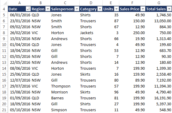
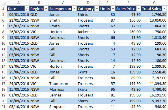
Let’s look at an example, below is our table of data:
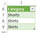
And we want to highlight the rows that contain any of the categories in this Table:
Like so:
Note: My list is in an Excel Table in cells I7:I9 and I’ve given it the Named Range: List. We’ll be using this name in the Conditional Formatting formula.
Download the Excel File
Enter your email address below to download the sample workbook.
By submitting your email address you agree that we can email you our Excel newsletter.
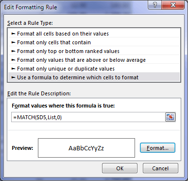
Step 1: To set up the Conditional Formatting we first select the Table cells we want to highlight, in my case A5:G47.
Step 2: Home tab > Conditional Formatting > New Rule > select ‘Use a formula to determine which cells to format’ from the Rule Type list.
Step 3: Insert the formula
=MATCH($D5,List,0)
In the dialog box as shown below:
Now if you remember my post from a couple of weeks ago with a similar example you’ll recall that I said Conditional Formatting formulas must always evaluate to TRUE or FALSE, or their numeric equivalents of 1 and 0.
And if you’re familiar with the MATCH Function you’ll know that it returns the position of a value in a list, and in this example that could be anything between 1 and 3. So you might be wondering how that MATCH formula works in Conditional Formatting.
Taking the formula above, it evaluates like so:
=MATCH($D5, List, 0)
=MATCH("Shirts", {"Shorts";"Shirts";"Skirts"}, 0)
=2
i.e. Shirts is the second item in the ‘List’.
So, the formula isn’t returning TRUE or FALSE, or their numeric equivalent of 1 and 0, yet the format is still applied. What?!
I discovered through experimenting that the conditional format will be applied as long as any (positive or negative) value other than zero is returned by the formula.
That means we could also use this formula to achieve the same results:
=COUNTIF(List, $D5)
Click here for a more thorough understanding of how Conditional Formatting formulas work.
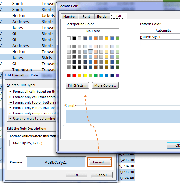
Step 4: Click the ‘Format’ button in the dialog box above and set your format:
Thanks
A big thank you to Cliff Beacham for sharing his ‘Excel Conditional Formatting Highlight Matches in List’ tip and for teaching me something new.
Cliff has an Excel book coming out soon. Keep your eye out on Amazon for it.
In this article, we will learn how to create a Dropdown list with color in Microsoft Excel.
Drop down list limits the user to choose a value from the list provided instead of adding values in sheet.
We will be using Conditional Formatting and Data Validation options.
First, let’s understand how to make a dropdown list in Excel with an example here

Here is a list of three colours Red, Green and Blue. We need that the user has to select from this list.
Click Data > Data Validation option in Excel 2016
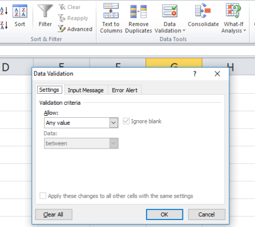
Data Validation dialog box appears as shown above.
Select the option List in Allow and select the source list in Source option and click OK.
A dropdown list will be created on the cell.
Now click Home > Conditional formatting. Select New rule from the list and a dialog box will appear.

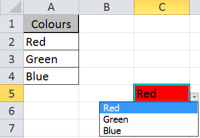
Select Specific Text option and select the cell for colour as in this case Red.
Select Format > Fill option. Select the Red colour and click OK.

Repeat the process for all the options like Green and Blue and your list will be shown like in below snapshot.
Drop down list and Conditional formatting tools are very useful in Excel 2016, to view your data in a particular format manner. You can create a dropdown list in google sheets using the same method.
If you liked our blogs, share it with your friends on Facebook. And also you can follow us on Twitter and Facebook.
We would love to hear from you, do let us know how we can improve, complement or innovate our work and make it better for you. Write us at info@exceltip.com
Check out more related articles:
How to edit a drop down list in Excel?
How to delete drop down list?
How to create dependent drop down list?
How to create multiple dropdown List without repetition using named ranges?
How to create drop down list?
Popular Articles:
50 Excel Shortcut to Increase Your Productivity
How to use the VLOOKUP Function in Excel
How to use the COUNTIF function in Excel 2016
How to use the SUMIF Function in Excel
Excel has some useful features that allow you to save time and be a lot more productive in your day-to-day work.
One such useful (and less-known) feature in the Custom Lists in Excel.
Now, before I get to how to create and use custom lists, let me first explain what’s so great about it.
Suppose you have to enter numbers the month names from Jan to Dec in a column. How would you do it? And no, doing it manually is not an option.
One of the fastest ways would be to have January in a cell, February in an adjacent cell and then use the fill handle to drag and let Excel automatically fill in the rest. Excel is smart enough to realize that you want to fill the next month in each cell in which you drag the fill handle.
Month names are quite generic and therefore it’s available by default in Excel.
But what if you have a list of department names (or employee names or product names), and you want to do the same. Instead of manually entering these or copy-paste these, you want these to appear magically when you use the fill handle (just like month names).
You can do that too…
… by using Custom Lists in Excel
In this tutorial, I will show you how to create your own custom lists in Excel and how to use these to save time.
How to Create Custom Lists in Excel
By default, Excel already has some pre-fed custom lists that you can use to save time.
For example, if you enter ‘Mon’ in one cell ‘Tue’ in an adjacent cell, you can use the fill handle to fill the rest of the days. In case you extend the selection, keep on dragging and it will repeat and give you the day’s name again.

Below are the custom lists that are already in-built in Excel. As you can see, these are mostly days and month names as these are fixed and will not change.

Now, suppose you want to create a list of departments that you often need in Excel, you can create a custom list for it. This way, the next time you need to get all the departments name in one place, you don’t need to rummage through old files. All you need to do is type the first two in the list and drag.

Below are the steps to create your own Custom List in Excel:
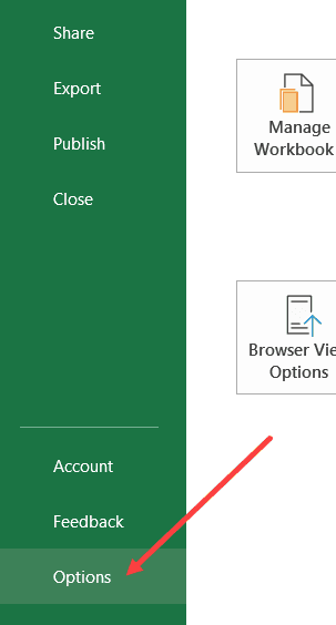
- Click the File tab

- Click on Options. This will open the ‘Excel Options‘ dialog box

- Click on the Advanced option in the left-pane

- In the General option, click on the ‘Edit Custom Lists’ button (you may have to scroll down to get to this option)

- In the Custom Lists dialog box, import the list by selecting the range of cells that have the list. Alternatively, you can also enter the name manually in the List Entries box (separated by comma or each name in a new line)

- Click on Add


As soon as you click on Add, you would notice that your list now becomes a part of the Custom Lists.

In case you have a large list that you want to add to Excel, you can also use the Import option in the dialog box.
Pro tip: You can also create a named range and use that named range to create the custom list. To do this, enter the name of the named range in the ‘Import list from cells’ field and click OK. The benefit of this is that you can change or expand the named range and it will automatically get adjusted as the custom list
Now that you have the list in Excel backend, you can use it just like you use numbers or month names with Autofill (as shown below).

While it’s great to be able to quickly get these custom lits names in Excel by doing a simple drag and drop, there is something even more awesome that you can do with custom lists (that’s what the next section is about).
Create Your Own Sorting Criteria Using Custom Lists
One great thing about custom lists is that you can use it to create your own sorting criteria. For example, suppose you have a dataset as shown below and you want to sort this based on High, Medium, and Low.

You can’t do this!
If you sort alphabetically, it would screw the alphabetical order (it will give you High, Low, and Medium and not High, Medium, and Low).
This is where Custom Lists really shine.
You can create your own list of items and then use these to sort the data. This way, you will get all the High values together at the top followed by the medium and low values.
The first step is to create a custom list (High, Medium, Low) using the steps shown in the previous section (‘How to Create Custom Lists in Excel‘).
Once you have the custom list created, you can use the below steps to sort based on it:
- Select the entire dataset (including the headers)
- Click the Data tab

- In the Sort and Filter group, click on the Sort icon. This will open the Sort dialog box

- In the Sort dialog box, make the following selections:
- Sort by Column: Priority
- Sort On: Cell Values
- Order: Custom Lists. When the dialog box opens, select the sorting criteria you want to use and then click on OK.

- Click OK


The above steps would instantly sort the data using the list you created and used as criteria while sorting (High, Medium, Low in this example).

Note that you don’t necessarily need to create the custom list first to use it in sorting. You can use the above steps and in Step 4 when the dialog box opens, you can create a list right there in that dialog box.
Some Examples Where you can Use Custom Lists
Below are some of the cases where creating and using custom lists can save you time:
- If you have a list that you need to enter manually (or copy-paste from some other source), you can create a custom list and use that instead. For example, this could be department names in your organization, or product names or regions/countries.
- If you’re a teacher, you can create a list of your student names. That way, when you are grading them the next time, you don’t need to worry about entering the student names manually or copy-pasting it from some other sheet. This also ensures that there are fewer chances of errors.
- When you need to sort data based on criteria that are not in-built in Excel. As covered in the previous section, you can use your own sorting criteria by making a custom list in Excel.
So this is all that you need to know about Creating Custom Lists in Excel.
I hope you found this useful.
You may also like the following Excel tutorials:
- How to Sort by the Last Name in Excel
- How to SORT in Excel (by Rows, Columns, Colors, Dates, & Numbers)
- How to Sort By Color in Excel
- How to Sort Worksheets in Excel
- Automatically Sort Data in Alphabetical Order using Formula
When we need to collect data from others, they may write different things from their perspective. Still, we need to make all the related stories under one. Also, it is common that while entering the data, they make mistakes because of typo errors. For example, assume in certain cells, if we ask users to enter either “YES” or “NO,” one will enter “Y,” someone will insert “YES” like this, and we may end up getting a different kind of results. So in such cases, creating a list of values as pre-determined values allows the users only to choose from the list instead of users entering their values. Therefore, in this article, we will show you how to create a list of values in Excel.
Table of contents
- Create List in Excel
- #1 – Create a Drop-Down List in Excel
- #2 – Create List of Values from Cells
- #3 – Create List through Named Manager
- Things to Remember
- Recommended Articles
You can download this Create List Excel Template here – Create List Excel Template
#1 – Create a Drop-Down List in Excel
We can create a drop-down list in Excel using the “Data Validation in excelThe data validation in excel helps control the kind of input entered by a user in the worksheet.read more” tool, so as the word itself says, data will be validated even before the user decides to enter. So, all the values that need to be entered are pre-validated by creating a drop-down list in Excel. For example, assume we need to allow the user to choose only “Agree” and “Not Agree,” so we will create a list of values in the drop-down list.
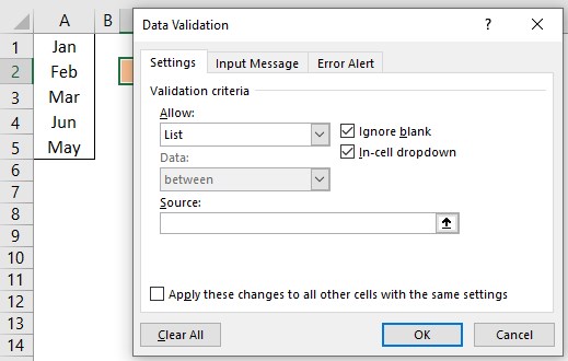
- In the Excel worksheet under the “Data” tab, we have an option called “Data Validation” from this again, choose “Data Validation.”

- As a result, this will open the “Data Validation” tool window.
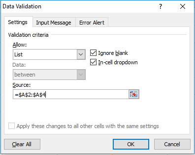
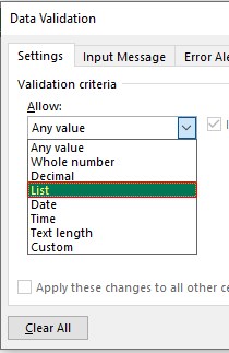
- The “Settings” tab will be shown by default, and now we need to create validation criteria. Since we are creating a list of values, choose “List” as the option from the “Allow” drop-down list.
- For this “List,” we can give a list of values to be validated in the following way, i.e., by directly entering the values in the “Source” list.

- Enter the first value as “Agree.”
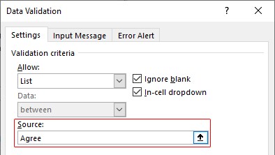
- Once the first value to be validated is entered, we need to enter “comma” (,) as the list separator before entering the next value. So, enter “comma” and enter the following values as “Not Agree.”
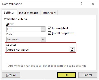
- After that, click on “Ok,” and the list of values may appear in the form of the “drop-down” list.

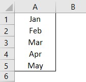
#2 – Create a List of Values from Cells
The above method is to get started, but imagine the scenario of creating a long list of values or your list of values changing now and then. Then, it may get difficult to return and edit the list of values manually. So, by entering values in the cell, we can easily create a list of values in Excel.
Follow the steps to create a list from cell values.
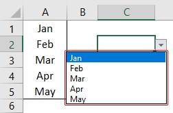
- We must first insert all the values in the cells.

- Then, open “Data Validation” and choose the validation type as “List.”

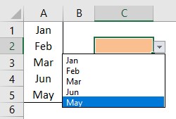
- Next, in the “Source” box, we need to place the cursor and select the list of values from the range of cells A1 to A5.

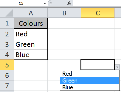
- Click on “OK,” and we will have the list ready in cell C2.

So values to this list are supplied from the range of cells A1 to A5. Any changes in these referenced cells will also impact the drop-down list.
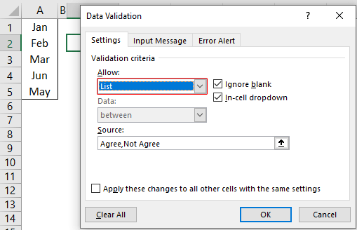
For example, in cell A4, we have a value as “Apr,” but now we will change that to “Jun” and see what happens in the drop-down list.
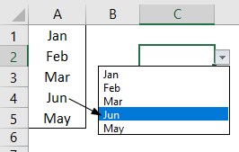
Now, look at the result of the drop-down list. Instead of “Apr,” we see “Jun” because we had given the list source as cell range, not manual entries.
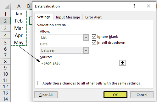
#3 – Create List through Named Manager
There is another way to create a list of values, i.e., through named ranges in excelName range in Excel is a name given to a range for the future reference. To name a range, first select the range of data and then insert a table to the range, then put a name to the range from the name box on the left-hand side of the window.read more.
- We have values from A1 to A5 in the above example, naming this range “Months.”

- Now, select the cell where we need to create a list and open the drop-down list.
- Now place the cursor in the “Source” box and press the F3 key to an open list of named ranges.
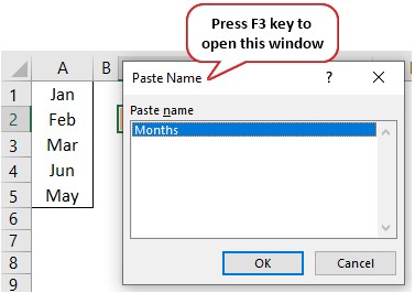
- As we can see above, we have a list of names, choose the name “Months” and click on “OK” to get the name to the “Source” box.
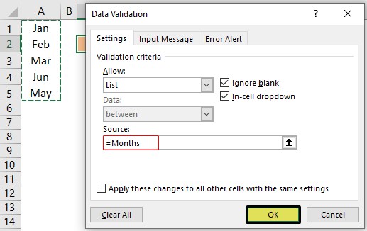
- Click on “OK,” and the drop-down list is ready.
Things to Remember
- The shortcut key to open data validation is “ALT + A + V + V.“
- We must always create a list of values in the cells so that it may impact the drop-down list if any change happens in the referenced cells.
Recommended Articles
This article has been a guide to Excel Create List. Here, we learn how to create a list of values in Excel also, create a simple drop-down method and make a list through name manager along with examples and downloadable Excel templates. You may learn more about Excel from the following articles: –
- Custom List in Excel
- Drop Down List in Excel
- Compare Two Lists in Excel
- How to Randomize List in Excel?