
Create a drop-down list
You can help people work more efficiently in worksheets by using drop-down lists in cells. Drop-downs allow people to pick an item from a list that you create.

-
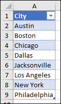
In a new worksheet, type the entries you want to appear in your drop-down list. Ideally, you’ll have your list items in an
Excel table
. If you don’t, then you can quickly convert your list to a table by selecting any cell in the range, and pressing
Ctrl+T
.
Notes:
-
Why should you put your data in a table? When your data is in a table, then as you
add or remove items from the list
, any drop-downs you based on that table will automatically update. You don’t need to do anything else. -
Now is a good time to
Sort data in a range or table
in your drop-down list.
-
-
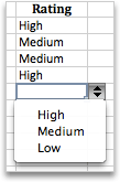
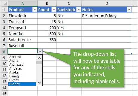
Select the cell in the worksheet where you want the drop-down list.
-
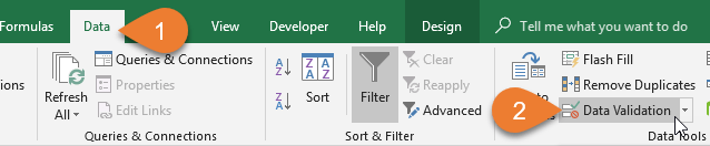
Go to the
Data
tab on the Ribbon, then
Data Validation
.Note:
If you can’t click
Data Validation
, the worksheet might be protected or shared.
Unlock specific areas of a protected workbook
or stop sharing the worksheet, and then try step 3 again. -
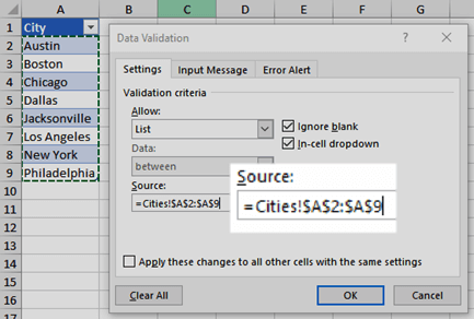
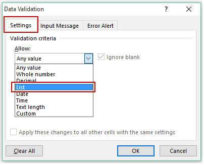
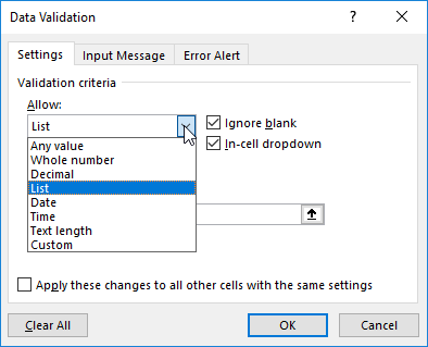
On the
Settings
tab, in the
Allow
box, click
List
. -
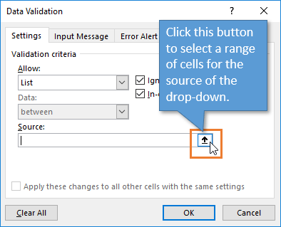
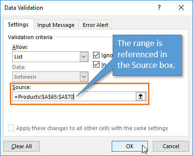
Click in the
Source
box, then select your list range. We put ours on a sheet called Cities, in range A2:A9. Note that we left out the header row, because we don’t want that to be a selection option:
-
If it’s OK for people to leave the cell empty, check the
Ignore blank
box. -
Check the
In-cell dropdown
box. -
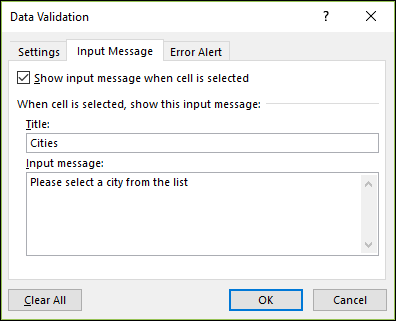
Click the
Input Message
tab.-
If you want a message to pop up when the cell is clicked, check the
Show input message when cell is selected
box, and type a title and message in the boxes (up to 225 characters). If you don’t want a message to show up, clear the check box.
-
-
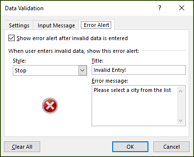
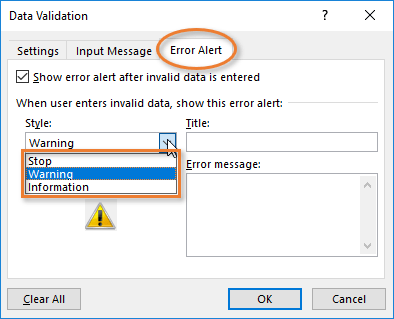
Click the
Error Alert
tab.-
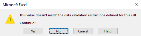
If you want a message to pop up when someone enters something that’s not in your list, check the
Show error alert after invalid data is entered
box, pick an option from the
Style
box, and type a title and message. If you don’t want a message to show up, clear the check box.
-
-
Not sure which option to pick in the
Style
box?-
To show a message that doesn’t stop people from entering data that isn’t in the drop-down list, click
Information
or Warning. Information will show a message with this icon
and Warning will show a message with this icon
. -
To stop people from entering data that isn’t in the drop-down list, click
Stop
.Note:
If you don’t add a title or text, the title defaults to «Microsoft Excel» and the message to: «The value you entered is not valid. A user has restricted values that can be entered into this cell.»
-


You can download an example workbook with multiple data validation examples like the one in this article. You can follow along, or create your own data validation scenarios.
Download Excel data validation examples
.
Data entry is quicker and more accurate when you restrict values in a cell to choices from a drop-down list.
Start by making a list of valid entries on a sheet, and sort or rearrange the entries so that they appear in the order you want. Then you can use the entries as the source for your drop-down list of data. If the list is not large, you can easily refer to it and type the entries directly into the data validation tool.
-
Create a list of valid entries for the drop-down list, typed on a sheet in a single column or row without blank cells.
-
Select the cells that you want to restrict data entry in.
-
On the
Data
tab, under
Tools
, click
Data Validation
or
Validate
.
Note:
If the validation command is unavailable, the sheet might be protected or the workbook may be shared. You cannot change data validation settings if your workbook is shared or your sheet is protected. For more information about workbook protection, see
Protect a workbook
. -
Click the
Settings
tab, and then in the
Allow
pop-up menu, click
List
. -
Click in the
Source
box, and then on your sheet, select your list of valid entries.The dialog box minimizes to make the sheet easier to see.
-
Press RETURN or click the
Expand
button to restore the dialog box, and then click
OK
.Tips:
-
You can also type values directly into the
Source
box, separated by a comma. -
To modify the list of valid entries, simply change the values in the source list or edit the range in the
Source
box. -
You can specify your own error message to respond to invalid data inputs. On the
Data
tab, click
Data Validation
or
Validate
, and then click the
Error Alert
tab.
-

See also
Apply data validation to cells
-
In a new worksheet, type the entries you want to appear in your drop-down list. Ideally, you’ll have your list items in an
Excel table
.Notes:
-
Why should you put your data in a table? When your data is in a table, then as you
add or remove items from the list
, any drop-downs you based on that table will automatically update. You don’t need to do anything else. -
Now is a good time to
Sort your data in the order you want it to appear
in your drop-down list.
-
-
Select the cell in the worksheet where you want the drop-down list.
-
Go to the
Data
tab on the Ribbon, then click
Data Validation
. -
On the
Settings
tab, in the
Allow
box, click
List
. -
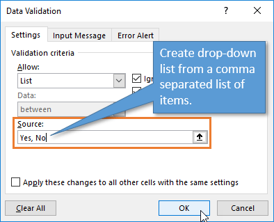
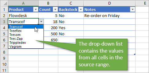
If you already made a table with the drop-down entries, click in the
Source
box, and then click and drag the cells that contain those entries. However, do not include the header cell. Just include the cells that should appear in the drop-down. You can also just type a list of entries in the
Source
box, separated by a comma like this:
Fruit,Vegetables,Grains,Dairy,Snacks
-
If it’s OK for people to leave the cell empty, check the
Ignore blank
box. -
Check the
In-cell dropdown
box. -
Click the
Input Message
tab.-
If you want a message to pop up when the cell is clicked, check the
Show message
checkbox, and type a title and message in the boxes (up to 225 characters). If you don’t want a message to show up, clear the check box.
-
-
Click the
Error Alert
tab.-
If you want a message to pop up when someone enters something that’s not in your list, check the
Show Alert
checkbox, pick an option in
Type
, and type a title and message. If you don’t want a message to show up, clear the check box.
-
-
Click
OK
.
After you create your drop-down list, make sure it works the way you want. For example, you might want to check to see if
Change the column width and row height
to show all your entries. If you decide you want to change the options in your drop-down list, see
Add or remove items from a drop-down list
. To delete a drop-down list, see
Remove a drop-down list
.
Need more help?
You can always ask an expert in the Excel Tech Community or get support in the Answers community.
See also
Add or remove items from a drop-down list
Video: Create and manage drop-down lists
Overview of Excel tables
Apply data validation to cells
Lock or unlock specific areas of a protected worksheet
Need more help?
A drop-down list is an excellent way to give the user an option to select from a pre-defined list.
It can be used while getting a user to fill a form, or while creating interactive Excel dashboards.
Drop-down lists are quite common on websites/apps and are very intuitive for the user.
Watch Video – Creating a Drop Down List in Excel
In this tutorial, you’ll learn how to create a drop down list in Excel (it takes only a few seconds to do this) along with all the awesome stuff you can do with it.
How to Create a Drop Down List in Excel
In this section, you will learn the exacts steps to create an Excel drop-down list:
- Using Data from Cells.
- Entering Data Manually.
- Using the OFFSET formula.
#1 Using Data from Cells
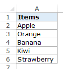
Let’s say you have a list of items as shown below:
Here are the steps to create an Excel Drop Down List:
- Select a cell where you want to create the drop down list.
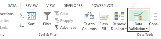
- Go to Data –> Data Tools –> Data Validation.

- In the Data Validation dialogue box, within the Settings tab, select List as the Validation criteria.
- As soon as you select List, the source field appears.

- As soon as you select List, the source field appears.
- In the source field, enter =$A$2:$A$6, or simply click in the Source field and select the cells using the mouse and click OK. This will insert a drop down list in cell C2.
- Make sure that the In-cell dropdown option is checked (which is checked by default). If this option in unchecked, the cell does not show a drop down, however, you can manually enter the values in the list.

- Make sure that the In-cell dropdown option is checked (which is checked by default). If this option in unchecked, the cell does not show a drop down, however, you can manually enter the values in the list.
Note: If you want to create drop down lists in multiple cells at one go, select all the cells where you want to create it and then follow the above steps. Make sure that the cell references are absolute (such as $A$2) and not relative (such as A2, or A$2, or $A2).
#2 By Entering Data Manually
In the above example, cell references are used in the Source field. You can also add items directly by entering it manually in the source field.
For example, let’s say you want to show two options, Yes and No, in the drop down in a cell. Here is how you can directly enter it in the data validation source field:
This will create a drop-down list in the selected cell. All the items listed in the source field, separated by a comma, are listed in different lines in the drop down menu.
All the items entered in the source field, separated by a comma, are displayed in different lines in the drop down list.
Note: If you want to create drop down lists in multiple cells at one go, select all the cells where you want to create it and then follow the above steps.
#3 Using Excel Formulas
Apart from selecting from cells and entering data manually, you can also use a formula in the source field to create an Excel drop down list.
Any formula that returns a list of values can be used to create a drop-down list in Excel.
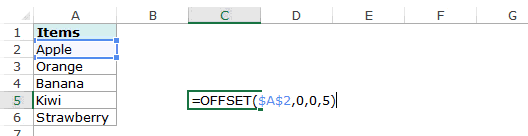
For example, suppose you have the data set as shown below:
Here are the steps to create an Excel drop down list using the OFFSET function:
This will create a drop-down list that lists all the fruit names (as shown below).
 Note: If you want to create a drop-down list in multiple cells at one go, select all the cells where you want to create it and then follow the above steps. Make sure that the cell references are absolute (such as $A$2) and not relative (such as A2, or A$2, or $A2).
How this formula Works??
In the above case, we used an OFFSET function to create the drop down list. It returns a list of items from the ra
It returns a list of items from the range A2:A6.
Here is the syntax of the OFFSET function: =OFFSET(reference, rows, cols, [height], [width])
It takes five arguments, where we specified the reference as A2 (the starting point of the list). Rows/Cols are specified as 0 as we don’t want to offset the reference cell. Height is specified as 5 as there are five elements in the list.
Now, when you use this formula, it returns an array that has the list of the five fruits in A2:A6. Note that if you enter the formula in a cell, select it and press F9, you would see that it returns an array of the fruit names.
Creating a Dynamic Drop Down List in Excel (Using OFFSET)
The above technique of using a formula to create a drop down list can be extended to create a dynamic drop down list as well. If you use the OFFSET function, as shown above, even if you add more items to the list, the drop down would not update automatically. You will have to manually update it each time you change the list.
Here is a way to make it dynamic (and it’s nothing but a minor tweak in the formula):
- Select a cell where you want to create the drop down list (cell C2 in this example).
- Go to Data –> Data Tools –> Data Validation.
- In the Data Validation dialogue box, within the Settings tab, select List as the Validation criteria. As soon as you select List, the source field appears.
- In the source field, enter the following formula: =OFFSET($A$2,0,0,COUNTIF($A$2:$A$100,”<>”))
- Make sure that the In-cell drop down option is checked.
- Click OK.
In this formula, I have replaced the argument 5 with COUNTIF($A$2:$A$100,”<>”).
The COUNTIF function counts the non-blank cells in the range A2:A100. Hence, the OFFSET function adjusts itself to include all the non-blank cells.
Note:
- For this to work, there must NOT be any blank cells in between the cells that are filled.
- If you want to create a drop-down list in multiple cells at one go, select all the cells where you want to create it and then follow the above steps. Make sure that the cell references are absolute (such as $A$2) and not relative (such as A2, or A$2, or $A2).
Copy Pasting Drop-Down Lists in Excel
You can copy paste the cells with data validation to other cells, and it will copy the data validation as well.
For example, if you have a drop-down list in cell C2, and you want to apply it to C3:C6 as well, simply copy the cell C2 and paste it in C3:C6. This will copy the drop-down list and make it available in C3:C6 (along with the drop down, it will also copy the formatting).
If you only want to copy the drop down and not the formatting, here are the steps:
This will only copy the drop down and not the formatting of the copied cell.
Caution while Working with Excel Drop Down List
You need to to be careful when you are working with drop down lists in Excel.
When you copy a cell (that does not contain a drop down list) over a cell that contains a drop down list, the drop down list is lost.
The worst part of this is that Excel will not show any alert or prompt to let the user know that a drop down will be overwritten.
How to Select All Cells that have a Drop Down List in it
Sometimes, it ‘s hard to know which cells contain the drop down list.
Hence, it makes sense to mark these cells by either giving it a distinct border or a background color.
Instead of manually checking all the cells, there is a quick way to select all the cells that have drop-down lists (or any data validation rule) in it.
This would instantly select all the cells that have a data validation rule applied to it (this includes drop down lists as well).
Now you can simply format the cells (give a border or a background color) so that visually visible and you don’t accidentally copy another cell on it.
Here is another technique by Jon Acampora you can use to always keep the drop down arrow icon visible. You can also see some ways to do this in this video by Mr. Excel.
Creating a Dependent / Conditional Excel Drop Down List
Here is a video on how to create a dependent drop-down list in Excel.
If you prefer reading over watching a video, keep reading.
Sometimes, you may have more than one drop-down list and you want the items displayed in the second drop down to be dependent on what the user selected in the first drop-down.
These are called dependent or conditional drop down lists.
Below is an example of a conditional/dependent drop down list:

In the above example, when the items listed in ‘Drop Down 2’ are dependent on the selection made in ‘Drop Down 1’.
Now let’s see how to create this.
Here are the steps to create a dependent / conditional drop down list in Excel:
Now, when you make the selection in Drop Down 1, the options listed in Drop Down List 2 would automatically update.
Download the Example File

How does this work? – The conditional drop down list (in cell E3) refers to =INDIRECT(D3). This means that when you select ‘Fruits’ in cell D3, the drop down list in E3 refers to the named range ‘Fruits’ (through the INDIRECT function) and hence lists all the items in that category.
Important Note While Working with Conditional Drop Down Lists in Excel:
- When you have made the selection, and then you change the parent drop down, the dependent drop down would not change and would, therefore, be a wrong entry. For example, if you select the US as the country and then select Florida as the state, and then go back and change the country to India, the state would remain as Florida. Here is a great tutorial by Debra on clearing dependent (conditional) drop down lists in Excel when the selection is changed.
- If the main category is more than one word (for example, ‘Seasonal Fruits’ instead of ‘Fruits’), then you need to use the formula =INDIRECT(SUBSTITUTE(D3,” “,”_”)), instead of the simple INDIRECT function shown above. The reason for this is that Excel does not allow spaces in named ranges. So when you create a named range using more than one word, Excel automatically inserts an underscore in between words. So ‘Seasonal Fruits’ named range would be ‘Seasonal_Fruits’. Using the SUBSTITUTE function within the INDIRECT function makes sure that spaces are converted into underscores.
You May Also Like the Following Excel Tutorials:
- Extract Data from Drop Down List Selection in Excel.
- Select Multiple Items from a Drop Down List in Excel.
- Creating a Dynamic Excel Filter Search Box.
- Display Main and Subcategory in Drop Down List in Excel.
- How to Insert Checkbox in Excel.
- Using a Radio Button (Option Button) in Excel.
- How to Remove Drop-Down List in Excel?
This post will show you everything there is to know about dropdown lists in Microsoft Excel.
If you are creating an Excel spreadsheet for other users to input data, then dropdown lists are very useful to control what data they are entering.
This way you can ensure that they will not enter incorrect data which will produce errors in your spreadsheet when calculations are made based on the user input.
Dropdown lists should be familiar as you will frequently find them on the web or while working in other applications.
They enhance the user experience as they make choice selection easy and help to standardize data entry.
This post is going to cover everything about dropdown lists in Microsoft Excel.
Are you ready for the ultimate resource guide to dropdown lists in Microsoft Excel? Get your copy of the example workbook and follow along!
Example Dataset
All the examples in this post will use the above standard set of data within Excel.
How to Create a Dropdown List
There are several ways to populate list items when you create a dropdown list within your spreadsheet.
Use Comma Separated List of Values for List Items
The first method is the most basic where all items are entered in the Data Validation menu as a comma-separated list.
- Go to the Data tab and click on the Data Validation button in the Data Tools group.
- This will open the Data Validation menu. Go to the Settings tab and select List from the Allow dropdown.
- In the Source input box, enter your delimited list using commas as the delimiter between items.
- Click OK button to create your dropdown list.
📝 Note: Keep the In-cell dropdown option checked as this is what will create the dropdown.
Your selected cell will now have a dropdown arrow to the right of it. Click the arrow, and your list will now show as separate items based on the comma delimiters that you entered.
📝 Note: If you use a comma and space to delimit your list items, Excel will remove the leading space from each item in your dropdown.
The advantage is that the list can be created in a very straightforward manner. All you need to do is to type the list in, or even paste it in from elsewhere.
The disadvantage is that it is hardcoded and is not dynamic. There is no way to change the list based on data entered in the spreadsheet.
Any changes to list items need to be done in the Data Validation menu. If you want to use the same list elsewhere in the spreadsheet, then you either need to copy and paste the list or set up the list from scratch.
Use a Range Reference for List Items
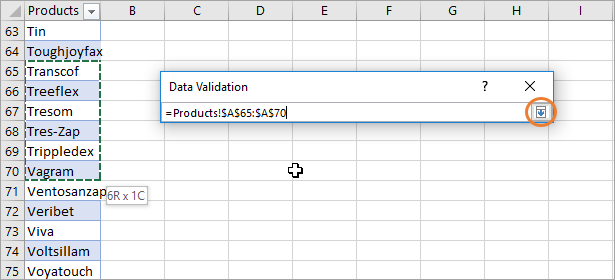
This is the most obvious choice for your list items as the Data Validation menu has a button to select a range from the grid.
From the Data Validation menu click on the Select button found on the right side of the Source input field. This will allow you to select the required range from the grid.
Use a Named Range for List Items
Another way to enter list items in your dropdown is by entering them in a named range, and then referencing the named range in the Data Validation menu.
Follow these steps to create a named range.
- Select the range of cells to use for the range name for the list of data that you want to use. This must be a single column range.
- Go to the Formula tab and click on the Define Name command in the Defined Names group of the ribbon. You can edit the range name afterward by clicking on Name Manager in the same group.
- This will open up the New Name menu. Enter a name for the range in the Name field. This is how you will refer to the range when creating a dropdown list.
- The cells you selected should be listed in the Refers to field, so check this is correct and update it if needed.
- Press the OK button.
This will create the name and when you select the range, you will see the name displayed in the Name Box.
You can also use the Name Box to skip the Define Name menu and quickly create a named range. Simply select the range of cells to name and then type the name into the Name Box and press Enter.
Now you can use the named range to create your dropdown list.
- Select the cell for your dropdown list.
- Go to the Data tab in the ribbon.
- Click on the Data Validation button in the Data Tools group.
- This will open up the Data Validation menu on the Settings tab. In the Allow dropdown, select List from the options.
- In the Source input box, enter the name of your named range for the list source. Precede it with an equal sign (=). You can also use the Up Arrow selector icon to select the range from the sheet. When you select the full named range, Excel will display the name as your selection.
- Press the OK button.
Your selected cell will now have a dropdown arrow to the right of it and will show all the items within your named range.
The advantage is that you can use this range name as a single source for many data validation lists. You can easily edit values in the named range, and that will reflect in all the dropdown lists that use that range.
Also, if the range name is moved to another location within the spreadsheet, it will still act as a valid source for all the dropdowns that use it as the source for list items.
The disadvantage is that you will need to set up the range name first of all, but if you have many dropdowns within the spreadsheet using this same source, then it is a very small overhead.
Use a Table for List Items
You can also use an Excel table as the source for your dropdown list.
Check out his post to find out everything about Excel tables if you haven’t seen them before.
Tables are great because it’s easy to add new data to the table. Just type in the row directly below the table and it will absorb the new data into the table.
New entries in the table will then appear in any dropdown lists with the table as a list item source.
Follow these steps to convert your range into a table.
- Select your data for the table including the header row.
- Go to the Insert tab and click on the Table button in the Tables group of the ribbon.
- This will open up the Create Table menu with the range selected. Make sure the My table has headers option is checked if your range had a column heading included. Press the OK button after you’ve checked everything is correct.
- Select the table go to the Table Design tab and give your new table a name. Type over the generic Table1 name with the new name and press Enter.
Now you will be able to create a dropdown list based on this table.
- Select the cell for your dropdown list and click on the Data Validation button in the Data tab.
- Select List in the Allow field.
= INDIRECT ( "Cars[Model]" )- Enter the above formula into the Source box. This assumes that your table is called Cars, and that Model is a column header in that table.
- Press the OK button.
Your selected cell will now have a dropdown list based on the Model column from your table.
Using a defined table has huge advantages over the previous methods described.
You can use a source that has multiple columns, and you can easily select which column you want to use by changing the header name within the source formula.
If you require separate dropdowns for both columns in the table, all you need to do is copy and paste the cell with the validation into another location, and alter the column name in the source formula.
This is easier than creating a separate single-column range name for each column of the data!
It is also easier for you to follow if you have several dropdowns all being driven off of one table. The table is also dynamic and can be easily changed or updated with new data that will automatically flow into the dropdown list.
📝 Note: If you change the table name, you will need to update the formula used in the Data Validation Source input to reflect the new name. This is because the name is referenced by a hard-coded text string.
Use a Dynamic Array Reference for Dropdown List Items
This is the most flexible method for adding list items in a dropdown list.
Start by adding a table containing your dropdown list of items. In an adjacent cell, insert a formula that references the entire column from the table.
=Cars[Model]In this example, the above formula has been entered in cell D3. You can see this creates an array that is the exact same as the table column that it references.
If you add, edit or delete any items in the table, the array will update accordingly to match.
You can then reference this dynamic array inside the Data Validation menu as =$D$3# the Source input. The hashtag means it will reference the entire array.
When you add, edit, or delete items in the table, items in the array will update. Because the dropdown list references the array, it will also update with the same changes.
How to Add Items to an Existing DropDown List
Once you have created dropdown lists you will probably need to make changes, such as adding, editing, or deleting items in the list.
In the example of cars that are used here, new models are frequently added, or older models are retired and might need to be removed.
Editing Dropdown List Items from a Comma Separated List
You can change the items in a dropdown list with the following steps.
- Select the cell which contains the dropdown list to edit.
- Go to the Data tab.
- Click on the Data Validation button in the Data Tools group of the ribbon.
- This will up the Data Validation menu and you can add, remove, or edit the list items in the Source input field.
- Press the OK button.
📝 Note: This will only update the items in the selected dropdown list. Other similar dropdown lists in the workbook will remain unchanged.
Editing Dropdown List Items from a Named Range
The data in the single column named range can be changed easily and will reflect through to any dropdown that uses that named range.
Adding a new item is a bit more involved as you will need to extend the named range. You can do this from the Name Manager.
- Go to the Formulas tab.
- Click on the Name Manager button in the Defined Names section.
- Select the named range to update.
- Update the range reference in the Refers to field to add more cells to the range.
- Click on the checkmark to the left of the Refers to field.
- Press the Close button.
The Named range will now include the cells which you added to the range reference and you can enter the new list items there.
Note: Unfortunately, typing new items at the bottom of your named range won’t automatically extend the named range. You need to update the range reference manually to ensure new items are included in your dropdown lists.
Editing Dropdown List Items from a Table
Because tables are dynamic, it is far easier to add, edit, or delete list items.
When you add a new item at the bottom of your table, the table will automatically expand to include the new row. This means your new item will appear in the dropdown list.
Editing or deleting an item is just as easy!
Type over any item in the table to edit it.
Right-click on an item and select Delete ➜ Table Rows. This will delete the entire row in the table and remove the item from the dropdown list.
Editing Dropdown List Items from a Dynamic Array
This is the exact same process as editing a dropdown list from a table.
Changes you make to the table will propagate to the dynamic array which drives the dropdown list.
How to Remove a Dropdown List
If you no longer require a particular dropdown list within your spreadsheet, it is very easily removed. Follow these steps to remove a dropdown list.
- Select the cell with the dropdown list to remove.
- Go to the Data tab.
- Click on Data Validation in the Data Tools group.
- Press the Clear All button in the Data Validation menu.
- Press the OK button.
This will only remove the dropdown list from the selected cell and not any other copies of the dropdown list.
Copy and Paste a Dropdown List
You may want to use your dropdown list elsewhere in the workbook and this can easily be done by copying and pasting the cell to a new location.
You can use the Paste Special command to paste in only the data validation in the cell.
Use Ctrl + C to copy the cell which contains the dropdown list.
Select the cell that you want to copy the dropdown to and then right-click on the cell, and choose Paste Special from the options.
You can also use the Ctrl + Alt + V keyboard shortcut to open the Paste Special menu.
The Paste Special menu will appear and you can select the Validation option and click on OK.
You will now have an exact copy of the dropdown list in your new cell and it will use the same source for its list items.
Create a Dropdown List from Another Sheet
If you want to copy and paste or cut and paste a dropdown list into a new sheet, you might run into a problem when the list items were created using a range reference.
If the range reference was originally created within the same sheet, then it won’t contain a reference to the sheet name.
='My Sheet'!$B$3:$B$12You will need to update the range reference with the sheet name like in the above example.
Search a Dropdown List in Excel Online
The online version of Excel has a handy feature that allows you to search the dropdown list by just typing in a few characters.
This will narrow down the available list of options to choose from in the dropdown. This is extremely useful when dealing with a long list of items!
For example, using the list of car models, you can type Ac into the cell and that will display all entries in the list beginning with Ac. In this case, it will display Accord and Accent.
In the case of a very long list, this could pull out several entries beginning with F.
As you enter more letters, the number of entries in the search list will decrease to list items with a partial match. You can then click on a value in the search list dropdown to select it.
Case Sensitive Dropdown List Items
You can make your dropdown list case sensitive by entering your list options as a comma separated text string.
If a user enters a value that does not correspond to an item in the list in both value and case, then an error message will appear.
This will ensure that the final value in the validation cell matches the case of the list items.
📝 Note: Any other source used for your list items will allow any variation of case to be entered into the cell.
Remove Duplicates from List Items
When you select data for list items, you may find that there are duplicates within that data.
Duplicates that are in the source data for the list items will show up in the list and there is no option in the Data Validation menu to remove them.
If you include them in the dropdown list, this can cause confusion for the user when they have multiple choices which are the same. It’s best to remove any duplicate values from the list of items.
How you remove the duplicate values will depend on whether your version of Excel has dynamic arrays.
Using a Dynamic Array
When you have dynamic arrays, getting a list of unique items is easy. You can use the UNIQUE function to return the items with the duplicates removed.
= UNIQUE ( Cars[Make] )You can use the above formula which references a table named Cars that contains a column named Make. This column contains a few repeated items.
Notice the UNIQUE function returns all the items from the table but does not repeat any item of them.
Now you can reference this dynamic array as the list of items for the dropdown list.
Sort List Items in a Dropdown List
The Data Validation menu gives no option to sort the list items into alphabetical order.
Sorting the list of items will help make finding an item in a long list much easier.
Fortunately, sorting list items can be done outside of the Data Validation menu and is a fairly easy implementation.
Using a Dynamic Array
With dynamic arrays, sorting is also quite easy. You can use the SORT function to sort your list items for the dropdown list.
= SORT ( Cars[Model] )The above formula can be used to sort a column in alphabetical order and the results can then be references in your dropdown list source input.
Edit All Dropdown Lists
When your spreadsheet has many exact copies of the same dropdown list, you may need to update them all when adding, editing, or deleting list items.
This is especially true when you are using drop-down lists with comma-separated list items.
Thankfully, there is an easy option to update all your dropdown lists at the same time.
Follow these steps to update all your dropdown lists that use the same settings.
- Select one of the dropdown lists to edit.
- Go to the Data tab.
- Select the Data Validation command in the Data Tools section.
- Make any changes to the Source list.
- Check the Apply these changes to all other cells with the same settings option.
- Press the OK button.
When you check this option in the Data Validation menu, you will see all dropdowns with the same settings will get selected in your sheet. When you press the OK button, the changes are made to all these cells.
Note: This will only affect dropdown lists in the current sheet! If you have dropdowns using the same settings but located in other sheets, then you will need to update those sheets separately.
Error Alerts for Dropdown Lists
The best thing about drop-down lists is they force users to input data correctly.
If a user tries to skip selection from the dropdown list and instead enter their own data, Excel will show a warning and entry will be prevented.
Data Validation for lists gives you the flexibility to change the default error alert message and also to change the icon used in the error message.
You can customize the error message in the Error Alert tab of the Data Validation menu.
- Make sure the Show error alert after invalid data is entered option is checked. It should be enabled by default.
- Select the Style of alert.
- Stop will prevent the user from entering any value not in the list.
- Warning will alert the user the item is not in the list, but will let them decide if they still want to enter the value or not.
- Information will only alert the user the item is not in the list but will keep the value entered.
- Add a Title for the alert.
- Add an Error message for the alert.
Press the OK button once you’ve adjusted the error alert settings to your liking.
Now when a user tries to enter a value into the cell which is not in the list, a pop-up alert will show with your custom message. The above example shows a Warning alert that gives the user the Yes or No option to continue with the entry.
Input Messages for Dropdown Lists
You can create an input message for your dropdown list. This will appear when the user selects the cell containing the dropdown list.
Click on the Input Message tab in the Data Validation pop-up window, and enter a title (optional) and a message for the user to see.
You can create an input message from the Input Message tab of the Data Validation menu.
- Make sure you check the option to Show input message when cell is selected. This will allow the pop-up to display when the cell is selected.
- Add a Title for the pop up message.
- Add the Input message to be displayed in the pop up.
Press the OK button to save the pop-up message on the dropdown list.
Now when you select the cell with the dropdown list, a pop-up will show with your custom message. This is a great way to add any required instructions for the spreadsheet user as it doesn’t even require the use of a dropdown.
Allow Entries Not in the Dropdown List Items
You may have a situation where you are using a dropdown in a cell, but you want to allow the user to enter values outside of the dropdown list.
This can be done from the Error Alert tab in the Data Validation menu.
Uncheck the Show error alert after invalid data is entered option.
This will give the user the option to use the dropdown list to select a value, but will not require it.
If a user does not pick from the list it will suppress the error message and allow any value to be entered in the cell.
Create a Dropdown List with VBA
Sub CreateDropdown()
    With Selection.Validation
        .Delete
        .Add Type:=xlValidateList, AlertStyle:=xlValidAlertStop, Operator:= _
        xlBetween, Formula1:="Yes, No, Maybe"
        .IgnoreBlank = True
        .InCellDropdown = True
        .InputTitle = ""
        .ErrorTitle = ""
        .InputMessage = ""
        .ErrorMessage = ""
        .ShowInput = True
        .ShowError = True
    End With
End Sub
You can use VBA to create a dropdown list.
The above VBA code can be used to create a basic dropdown from a comma separated list of items.
Create a Dropdown List with Office Scripts
function main(workbook: ExcelScript.Workbook) {
	let selectedSheet = workbook.getActiveWorksheet();

	selectedSheet.getRange("B2").getDataValidation().setRule({ list: { inCellDropDown: true, source: "Yes, No, Maybe" }});
	selectedSheet.getRange("B2").getDataValidation().setPrompt({ showPrompt: true, message: "", title: "" });
	selectedSheet.getRange("B2").getDataValidation().setErrorAlert({ showAlert: true, style: ExcelScript.DataValidationAlertStyle.stop, message: "", title: "" });
	selectedSheet.getRange("B2").getDataValidation().setIgnoreBlanks(true);
}
You can use Office Scripts to create a dropdown list.
The above TypeScript code can be used to create dropdown list based on a comma separated set of list items.
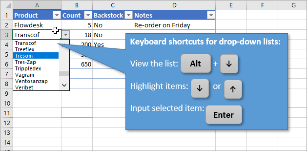
Keyboard Shortcuts for Using Dropdown Lists
There are useful keyboard shortcuts that you can use in conjunction with a Data Validation dropdown list.
- Alt + Down Arrow will activate the dropdown list and is the same as clicking the down arrow on the control.
- Up and Down Arrow keys will allow you to navigate and move up and down the dropdown list during selection.
- Enter will choose the item value that is highlighted in the dropdown list.
- Alt + A, V, V will take you straight to the Data Validation menu.
You can customize the QAT by adding your favorite commands so they are easily accessible at all times.
This will allow you to create your own keyboard shortcuts because every command you add to the QAT will get its own keyboard shortcut based on its position.
For example, the second command in your QAT can be used by pressing Alt + 2 on your keyboard.
This means you can add the Data Validation command to the QAT and access it with a customized keyboard shortcut.
Go to the Data tab and right-click on the Data Validation command. Select Add to Quick Access Toolbar from the menu and the command will be added to your QAT.
In this example, the data validation command is the third item in the QAT so you can press Alt + 3 to access it with the keyboard.
When you press the Alt key, the hotkey labels will show you what key to press next in order to access the commands.
Create a Dropdown List from Data Above the Current Cell
A useful feature in Excel is the ability to create a dropdown list from the data directly above the current cell.
- Select the cell directly below a column of data values.
- Right-click on the cell and select Pick From Drop-down List.
A dropdown will be instantly created in that cell based on the values above. The nice thing about this feature is it will only show a list of unique values and they will be sorted in alphabetical order.
The downside is that the dropdown list is not permanent, and the user has to right-click the cell again each time they want to use it.
Find All Dropdown Lists in a Sheet with Go To Special
Data Validation dropdown lists are hard to find within an Excel workbook. They remain invisible until the cell is selected, and the selector key appears to the right of the cell.
There is a way of highlighting all data validation cells on a spreadsheet.
- Select a cell that contains the dropdown list you want to find.
- Go to the Home tab.
- Select Find & Select from the Editing section.
- Select Go To Special to open up the Go To Special menu.
You can also press F5 and the Go To window will open, then you can press the Special button to open the Go To Special menu.
- Select the Data Validation option.
- Select Same from the Data Validation options.
- Press the OK button.
This will select all the cells in the sheet with the exact same data validation. This means it will differentiate between lists with slightly different list items!
📝 Note: The All option will find and select other types of data validations in the sheet and not just lists.
Dropdown List Template Tutorial
Dropdowns are so important and so widely used in Excel, that there is a dedicated tutorial template for dropdown lists which can be accessed from the File menu.
Go to the File tab and click on the Drop-down tutorial template then click on the Create button.
This template will take you on a guided and interactive tour of dropdown lists.
You can also download the template here.
Conclusions
Very often the wrong input can lead to errors in your spreadsheets.
Data Validation dropdown lists are very useful, for guiding or restricting a user as to what input they can use in certain cells to help avoid errors.
There are many ways of constructing dropdown lists, including from a comma-separated list, a range, a named range, a table, or a dynamic array.
A simple dropdown list is usually all that is required in most cases, but advanced setups such as dependent lists can be achieved with a bit of effort.
Advanced options are also available with your dropdown lists such as input messages and error alerts.
These all make dropdowns a versatile tool you need to start using in your spreadsheet solutions.
Are you using dropdown lists in your Excel workbooks? Do you have any special dropdown list tips I missed? Let me know in the comments below!
About the Author
John is a Microsoft MVP and qualified actuary with over 15 years of experience. He has worked in a variety of industries, including insurance, ad tech, and most recently Power Platform consulting. He is a keen problem solver and has a passion for using technology to make businesses more efficient.
Bottom Line: The complete Excel guide on how to create drop-down lists in cells (data validation lists). Includes keyboard shortcuts to select items, copying drop-downs to other cells, handling invalid inputs, updating lists with new items, and more.
Skill Level: Beginner
Download the Excel File
You can download the file I’m using in the video here:
What Are Data Validation Lists?
Creating a drop-down list is a great way to ensure that entries are uniform and free from spelling errors. It also helps restrict entries so that only values you’ve approved make it onto the sheet.
That’s why they are also called data validation lists. They help to make sure that only valid data makes it into the cells that you’ve applied it to.
This can be helpful when multiple users are entering data on the same sheet and you want the options to be limited to a list of items or values that you’ve already approved.
We can also use drop-down lists to create interactive reports and financial models, where results change when the user changes a cell’s value.
How to Create a Drop-down (Data Validation) List
To create a drop-down list, start by going to the Data tab on the Ribbon and click the Data Validation button.
The Data Validation window will appear. The keyboard shortcut to open the Data Validation window is Alt, A, V, V.
You’ll want to select List in the drop-down menu under Allow.
At this point there are a few ways that you can tell Excel what items you want to include in your drop-down list.
Drop-down List from Comma Separated Values
The first way is by typing all of the options that you want in your drop-down list, separated by commas, into the Source field. For example, if there are only two options to choose from, such as Yes and No, you would simply type “Yes, No” (do not include the quotation marks) in the Source box. It doesn’t matter whether a space follows your comma or not.
A longer list of options might look like this: “Red, Blue, Green, Purple, Orange, Yellow, Brown”. The options in your drop-down list will appear in the exact same order that you have typed them.
Note: On some language versions of Excel you will need to use a semicolon (;) instead of a comma.
Drop-down List from a Range of Values
The second way to fill your list with options is to choose them from a range of values. To do this, instead of typing values into the Source field, you want to select the icon to the right.
Selecting this icon will open up a small window that will auto-fill when you select a range of cells on the worksheet. Once you’ve selected the values you want to appear in your drop-down list, you can click on the corresponding icon to take you back to the Data Validation window.
At this point, the range you’ve selected will show in the Source box and you can just hit OK.
Now the values in the range that you’ve selected show as options that you can choose from in your drop-down list.
Shortcut for Selecting from the Drop-down List
To choose the option you want from your drop-down list, you can use your mouse to click on the option you want. Another way to select it is to use the keyboard shortcut Alt+?. This brings up the drop-down list and you can use your up and down arrow keys to highlight the selection you want, and then press Enter to select.
How to Search the Drop-down List
Unfortunately, Excel doesn’t have an option to search the drop-down list for a particular item, but I’ve created an add-in that gives you that option. It’s called List Search and you can access that add-in here:

Click here to download the List Search Add-in
Note: You will create a free account for the Excel Campus Members site to access the download and any future updates. The download site also contains installation instructions and videos.
How to Copy the Data Validation List to Other Cells
If you have created a drop-down list for a particular cell and would like other cells to have the same data validation list, you can easily copy (extend) that list to other cells.
Start by clicking on the cell that has the list, and then select any additional cells that you want to extend the drop-down list to. This can include blank cells or cells that already have values in them.
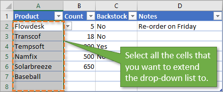
As before, you will click on the Data Validation button in the Data tab, but this time a warning will appear that says, “The selection contains some cells without Data Validation settings. Do you want to extend the Data Validation to these cells?”
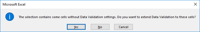
Choose Yes, and then hit OK when the Data Validation Window appears. You’ll see that each of the cells in your selection now has the same drop-down options as the original cell.
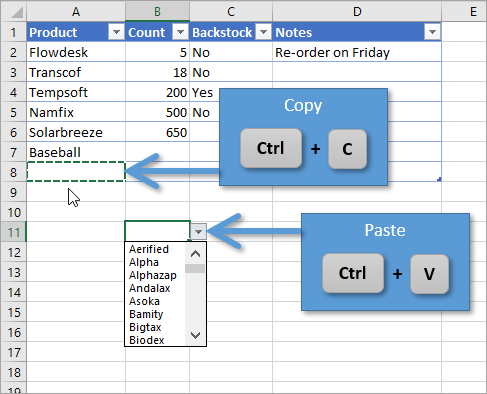
It’s also worth noting that you can copy and paste Data Validation from one cell to another just as you would copy and paste normal values and formatting.
Handling Errors and Invalid Inputs
What happens when we enter a value into a cell that has a Data Validation List, but that value is not one of the options in the list? That depends on the Error Alert settings, which we have control of.
To change the kind of message the user receives when they enter an extraneous value, you can go back to the Data Validation window. Under the Error Alert tab, you can find three options: Stop, Warning, and Information.
You’ll also notice that there are fields where you can change the title of the error message and the text of the message itself, so that when the user enters data that’s not part of your validation list, they will receive an alert that’s worded in the way you want it to appear.
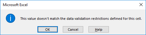
Here is an explanation of each Error Alert Style:
Stop Style
When the user types an invalid entry, an error message will appear that gives the option to either retype the entry or cancel the attempt. The message looks like this:

Warning Style
The Warning style displays a message that gives the user a choice to allow an entry that isn’t on the preset list.
Information Style
The Information style displays a message that automatically allows the entry no matter what the value is. The user is presented with informative text about validation rules.
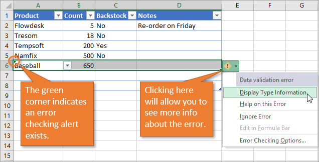
Error Checking Alert
When any invalid entry is made in a cell, the error checking alert will appear in the cell. The error is indicated with the green triangle in the top-left corner of the cell. Clicking the Error Box button will allow you to see more info about data validation error. You can select “Display Type Information” from the list to see the cause of the error.
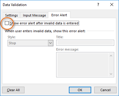
Disable Error Alerts
Another option under the Error Alert tab is to uncheck the box that says, “Show error alert after invalid data is entered.” This allows any value to be entered into the cell, and no message box will appear.
Adding New Data to the Source Range of the List
Adding new options to our drop-down list is possible, but it isn’t automatic when we add new items the bottom of our source list. We need to tell Excel what our new extended source range is. You can do that in the Data Validation window by just typing in the new range, or re-selecting the range to include the new data. (See the section above entitled “Create a Drop-Down List from a Range of Values” for how to select your range.)
The great thing is that we don’t have to redefine these settings for each cell that has Data Validation. The “Apply these changes to all other cells with the same settings” checkbox does this for us. When you click the checkbox, the other cells will selected in the background. This gives you a visual indication of what will be updated.
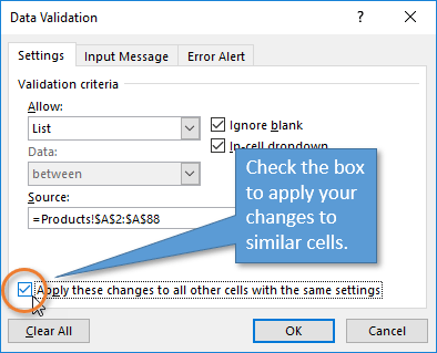
Then press OK. Any cells that shared the same data validation settings will now include the updated changes that you’ve made.
There is a way to automate the process so that any change you make to the source data instantly updates your drop-down list. It involves using Excel tables and named ranges. You can find out how in this post:
How to Add New Rows to Drop-down Lists Automatically – Dynamic Data Validation Lists
Removing Data Validation from a Cell
Getting rid of a Data Validation list is simple. Open the Data Validation window and click the Clear All button.
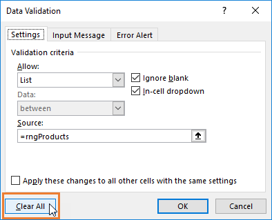
If you want to clear the validation settings from other cells with the same settings, make sure to click that checkbox before hitting the Clear All button.
Make Your Workbooks Interactive
Data Validation lists are a great tool to add to your Excel toolbelt. They help us keep our data clean and make our spreadsheets easier to use. We can use them as the source of lookup formulas to create interactive financial models and reports. I will do some follow-up posts with these techniques as well.
Once you feel comfortable with drop-down lists, you may want to try dependent (also called cascading) lists. These are lists that change depending on what you’ve already chosen in another list. For example, you may create a list of car brands, like Toyota, Ford, and Honda. Then you can have a second list of car models that populates with specific options depending on what you choose in the first list. If you choose Toyota in the first list, you might see Corolla, Camry, and Tacoma in the second. But if you go back to the first list and choose Ford, the options in the second list can change to Mustang, Explorer, and Focus. Learn how to create dependent cascading lists here.
If you have any questions or comments about how to use drop-down lists, don’t hesitate to leave a comment below. Thanks! 😊
Create a Drop-down List | Allow Other Entries | Add/Remove Items | Dynamic Drop-down List | Remove a Drop-down List | Dependent Drop-down Lists | Table Magic
Drop-down lists in Excel are helpful if you want to be sure that users select an item from a list, instead of typing their own values.
Create a Drop-down List
To create a drop-down list in Excel, execute the following steps.
1. On the second sheet, type the items you want to appear in the drop-down list.

Note: if you don’t want users to access the items on Sheet2, you can hide Sheet2. To achieve this, right click on the sheet tab of Sheet2 and click on Hide.
2. On the first sheet, select cell B1.

3. On the Data tab, in the Data Tools group, click Data Validation.

The ‘Data Validation’ dialog box appears.
4. In the Allow box, click List.
5. Click in the Source box and select the range A1:A3 on Sheet2.

6. Click OK.
Result:

Note: to copy/paste a drop-down list, select the cell with the drop-down list and press CTRL + c, select another cell and press CTRL + v.
7. You can also type the items directly into the Source box, instead of using a range reference.

Note: this makes your drop-down list case sensitive. For example, if a user types yes, an error alert will be displayed.
Allow Other Entries
You can also create a drop-down list in Excel that allows other entries.
1. First, if you type a value that is not in the list, Excel shows an error alert.

To allow other entries, execute the following steps.
2. On the Data tab, in the Data Tools group, click Data Validation.
The ‘Data Validation’ dialog box appears.
3. On the Error Alert tab, uncheck ‘Show error alert after invalid data is entered’.

4. Click OK.
5. You can now enter a value that is not in the list.

Add/Remove Items
You can add or remove items from a drop-down list in Excel without opening the ‘Data Validation’ dialog box and changing the range reference. This saves time.
1. To add an item to a drop-down list, go to the items and select an item.

2. Right click, and then click Insert.

3. Select «Shift cells down» and click OK.

Result:

Note: Excel automatically changed the range reference from Sheet2!$A$1:$A$3 to Sheet2!$A$1:$A$4. You can check this by opening the ‘Data Validation’ dialog box.
4. Type a new item.

Result:

5. To remove an item from a drop-down list, at step 2, click Delete, select «Shift cells up» and click OK.
Dynamic Drop-down List
You can also use a formula that updates your drop-down list automatically when you add an item to the end of the list.
1. On the first sheet, select cell B1.
2. On the Data tab, in the Data Tools group, click Data Validation.
The ‘Data Validation’ dialog box appears.
3. In the Allow box, click List.
4. Click in the Source box and enter the formula: =OFFSET(Sheet2!$A$1,0,0,COUNTA(Sheet2!$A:$A),1)

Explanation: the OFFSET function takes 5 arguments. Reference: Sheet2!$A$1, rows to offset: 0, columns to offset: 0, height: COUNTA(Sheet2!$A:$A) and width: 1. COUNTA(Sheet2!$A:$A) counts the number of values in column A on Sheet2 that are not empty. When you add an item to the list on Sheet2, COUNTA(Sheet2!$A:$A) increases. As a result, the range returned by the OFFSET function expands and the drop-down list will be updated.
5. Click OK.
6. On the second sheet, simply add a new item to the end of the list.

Result:

Remove a Drop-down List
To remove a drop-down list in Excel, execute the following steps.
1. Select the cell with the drop-down list.

2. On the Data tab, in the Data Tools group, click Data Validation.
The ‘Data Validation’ dialog box appears.
3. Click Clear All.

Note: to remove all other drop-down lists with the same settings, check «Apply these changes to all other cells with the same settings» before you click on Clear All.
4. Click OK.
Dependent Drop-down Lists
Want to learn even more about drop-down lists in Excel? Learn how to create dependent drop-down lists.
1. For example, if the user selects Pizza from a first drop-down list.

2. A second drop-down list contains the Pizza items.

3. But if the user selects Chinese from the first drop-down list, the second drop-down list contains the Chinese dishes.

Table Magic
You can also store your items in an Excel table to create a dynamic drop-down list.
1. On the second sheet, select a list item.

2. On the Insert tab, in the Tables group, click Table.

3. Excel automatically selects the data for you. Click OK.

4. If you select the list, Excel reveals the structured reference.

5. Use this structured reference to create a dynamic drop-down list.

Explanation: the INDIRECT function in Excel converts a text string into a valid reference.
6. On the second sheet, simply add a new item to the end of the list.

Result:
Note: try it yourself. Download the Excel file and create this drop-down list.
7. When using tables, use the UNIQUE function in Excel 365/2021 to extract unique list items.

Note: this dynamic array function, entered into cell F1, fills multiple cells. Wow! This behavior in Excel 365/2021 is called spilling.
8. Use this spill range to create a magic drop-down list.

Explanation: always use the first cell (F1) and a hash character to refer to a spill range.
Result:

Note: when you add new records, the UNIQUE function automatically extracts new unique list items and Excel automatically updates the drop-down list.
Содержание
- Создание дополнительного списка
- Создание выпадающего списка с помощью инструментов разработчика
- Связанные списки
- Вопросы и ответы

При работе в программе Microsoft Excel в таблицах с повторяющимися данными, очень удобно использовать выпадающий список. С его помощью можно просто выбирать нужные параметры из сформированного меню. Давайте выясним, как сделать раскрывающийся список различными способами.
Создание дополнительного списка
Самым удобным, и одновременно наиболее функциональным способом создания выпадающего списка, является метод, основанный на построении отдельного списка данных.
Прежде всего, делаем таблицу-заготовку, где собираемся использовать выпадающее меню, а также делаем отдельным списком данные, которые в будущем включим в это меню. Эти данные можно размещать как на этом же листе документа, так и на другом, если вы не хотите, чтобы обе таблице располагались визуально вместе.
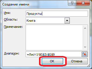
Выделяем данные, которые планируем занести в раскрывающийся список. Кликаем правой кнопкой мыши, и в контекстном меню выбираем пункт «Присвоить имя…».
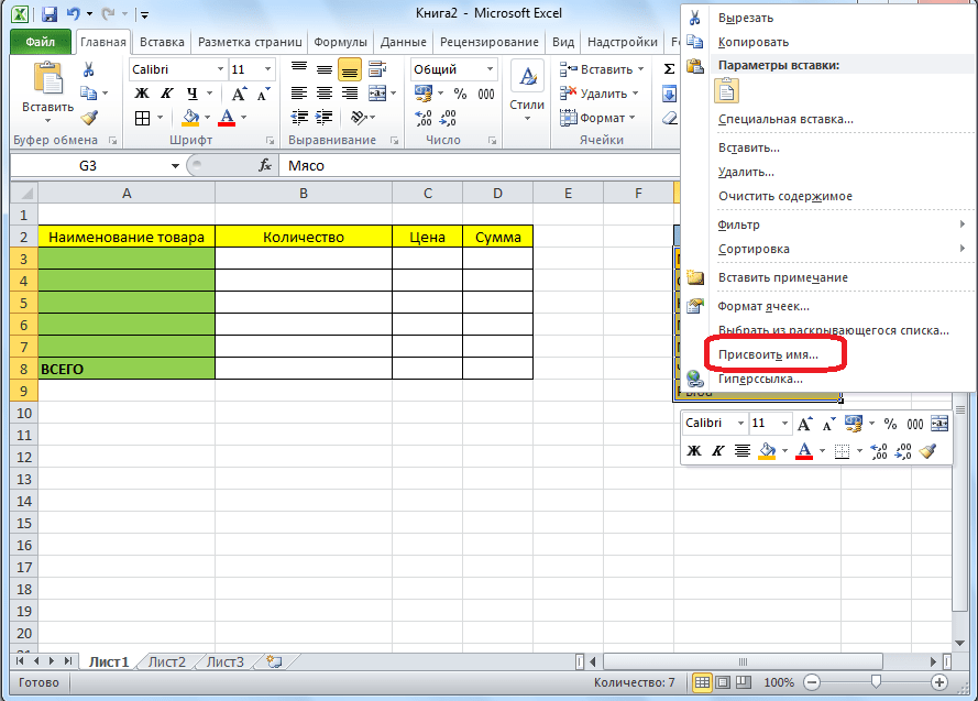
Открывается форма создания имени. В поле «Имя» вписываем любое удобное наименование, по которому будем узнавать данный список. Но, это наименование должно начинаться обязательно с буквы. Можно также вписать примечание, но это не обязательно. Жмем на кнопку «OK».
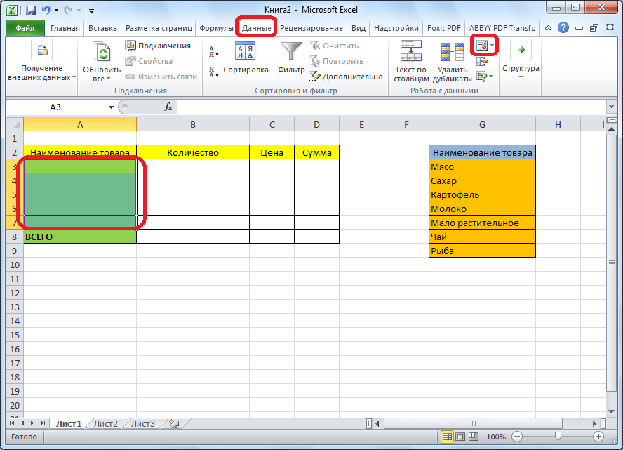
Переходим во вкладку «Данные» программы Microsoft Excel. Выделяем область таблицы, где собираемся применять выпадающий список. Жмем на кнопку «Проверка данных», расположенную на Ленте.
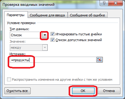
Открывается окно проверки вводимых значений. Во вкладке «Параметры» в поле «Тип данных» выбираем параметр «Список». В поле «Источник» ставим знак равно, и сразу без пробелов пишем имя списка, которое присвоили ему выше. Жмем на кнопку «OK».
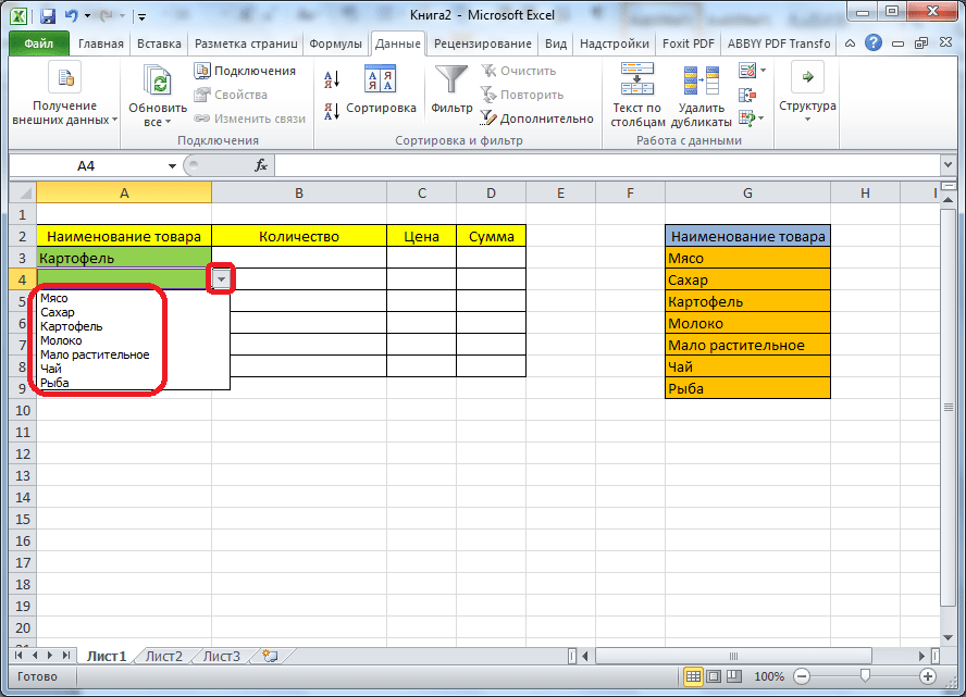
Выпадающий список готов. Теперь, при нажатии на кнопку у каждой ячейки указанного диапазона будет появляться список параметров, среди которых можно выбрать любой для добавления в ячейку.

Создание выпадающего списка с помощью инструментов разработчика
Второй способ предполагает создание выпадающего списка с помощью инструментов разработчика, а именно с использованием ActiveX. По умолчанию, функции инструментов разработчика отсутствуют, поэтому нам, прежде всего, нужно будет их включить. Для этого, переходим во вкладку «Файл» программы Excel, а затем кликаем по надписи «Параметры».
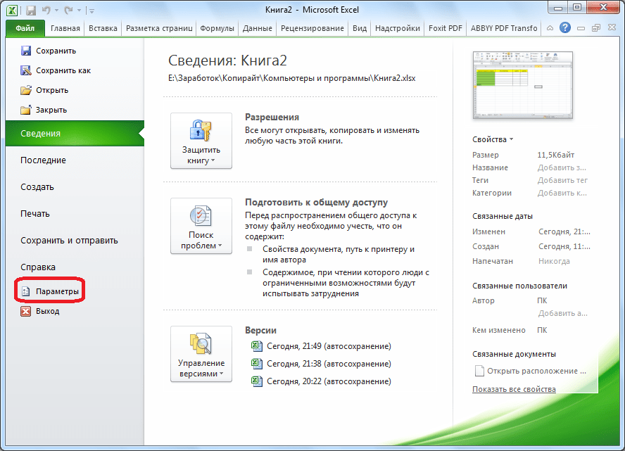
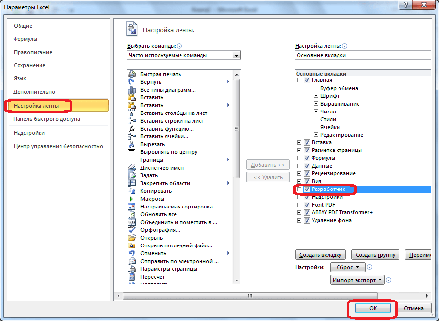
В открывшемся окне переходим в подраздел «Настройка ленты», и ставим флажок напротив значения «Разработчик». Жмем на кнопку «OK».
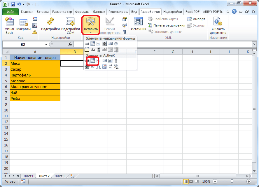
После этого, на ленте появляется вкладка с названием «Разработчик», куда мы и перемещаемся. Чертим в Microsoft Excel список, который должен стать выпадающим меню. Затем, кликаем на Ленте на значок «Вставить», и среди появившихся элементов в группе «Элемент ActiveX» выбираем «Поле со списком».
Кликаем по месту, где должна быть ячейка со списком. Как видите, форма списка появилась.
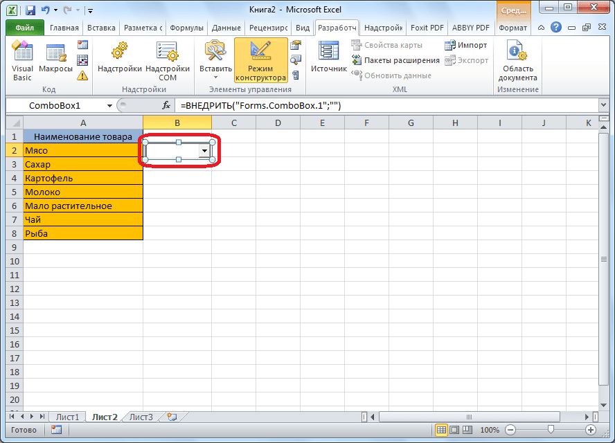
Затем мы перемещаемся в «Режим конструктора». Жмем на кнопку «Свойства элемента управления».
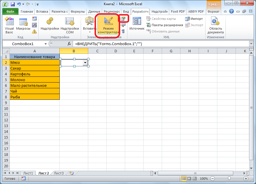
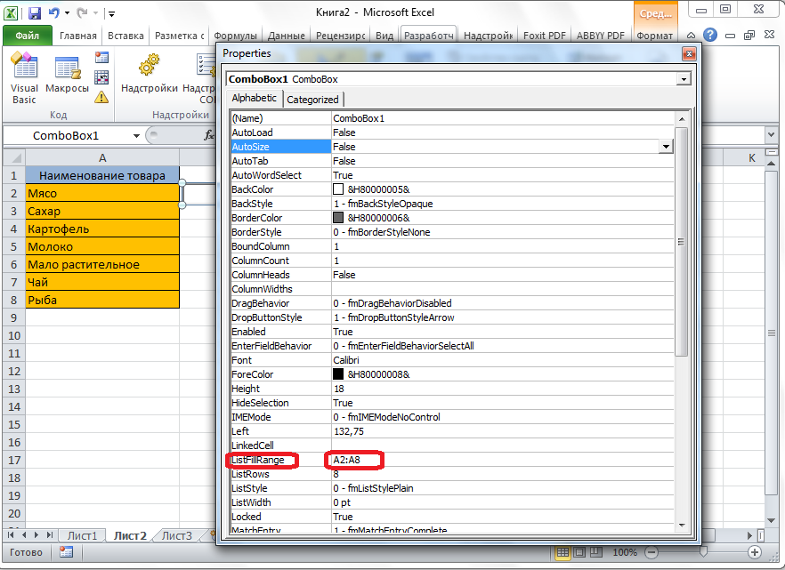
Открывается окно свойств элемента управления. В графе «ListFillRange» вручную через двоеточие прописываем диапазон ячеек таблицы, данные которой будут формировать пункты выпадающего списка.
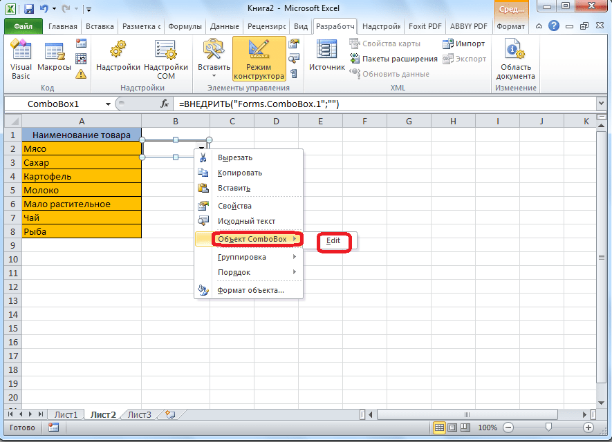
Далее, кликаем по ячейке, и в контекстном меню последовательно переходим по пунктам «Объект ComboBox» и «Edit».
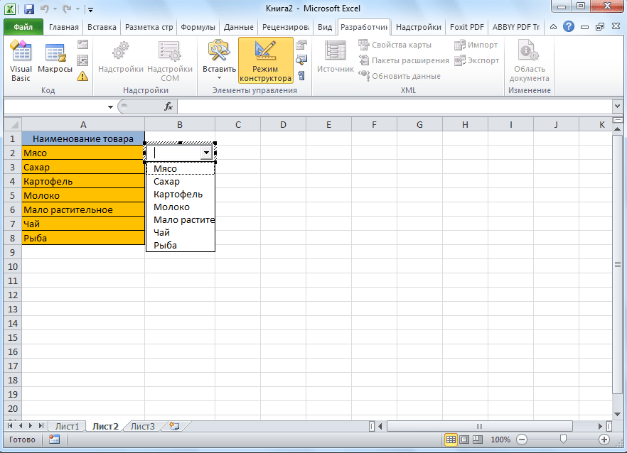
Выпадающий список в Microsoft Excel готов.
Чтобы сделать и другие ячейки с выпадающим списком, просто становимся на нижний правый край готовой ячейки, нажимаем кнопку мыши, и протягиваем вниз.
Связанные списки
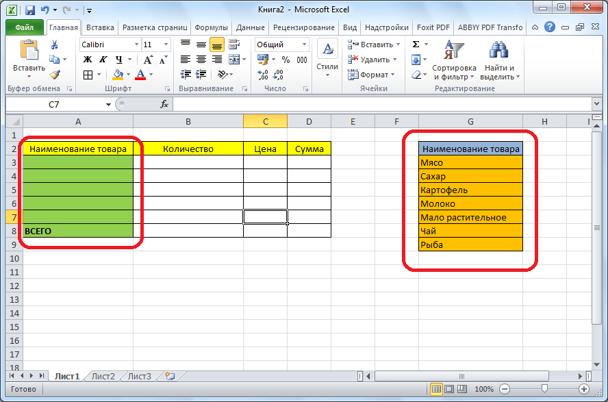
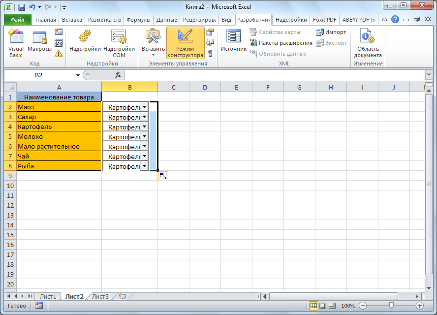
Также, в программе Excel можно создавать связанные выпадающие списки. Это такие списки, когда при выборе одного значения из списка, в другой графе предлагается выбрать соответствующие ему параметры. Например, при выборе в списке продуктов картофеля, предлагается выбрать как меры измерения килограммы и граммы, а при выборе масла растительного – литры и миллилитры.
Прежде всего, подготовим таблицу, где будут располагаться выпадающие списки, и отдельно сделаем списки с наименованием продуктов и мер измерения.
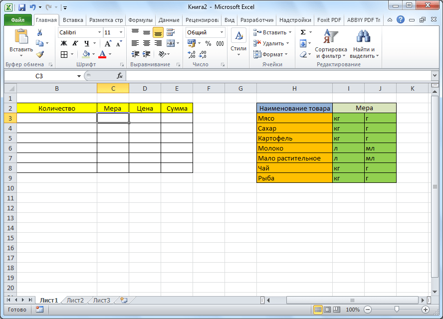
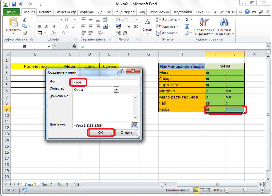
Присваиваем каждому из списков именованный диапазон, как это мы уже делали ранее с обычными выпадающими списками.
В первой ячейке создаём список точно таким же образом, как делали это ранее, через проверку данных.
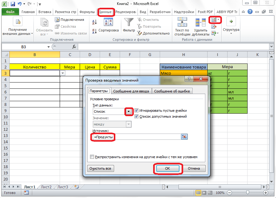
Во второй ячейке тоже запускаем окно проверки данных, но в графе «Источник» вводим функцию «=ДВССЫЛ» и адрес первой ячейки. Например, =ДВССЫЛ($B3).
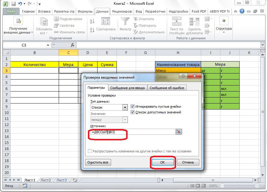
Как видим, список создан.
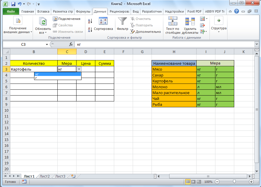
Теперь, чтобы и нижние ячейки приобрели те же свойства, как и в предыдущий раз, выделяем верхние ячейки, и при нажатой клавише мышки «протаскиваем» вниз.
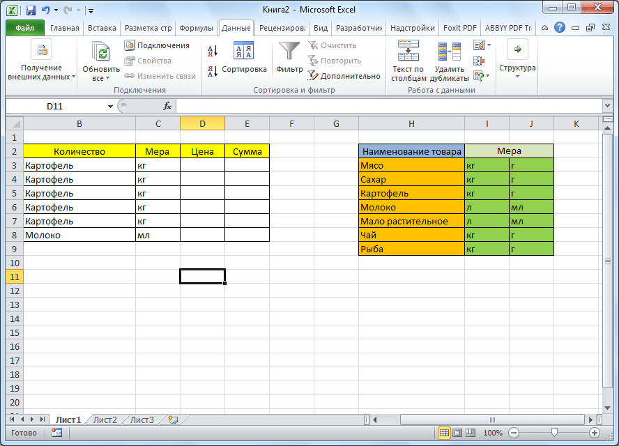
Всё, таблица создана.
Мы разобрались, как сделать выпадающий список в Экселе. В программе можно создавать, как простые выпадающие списки, так и зависимые. При этом, можно использовать различные методы создания. Выбор зависит от конкретного предназначения списка, целей его создания, области применения, и т.д.
Содержание
- 0.1 Простейший способ
- 0.1.1 Excel
- 0.1.2 Calc
- 0.2 Простейший способ
- 0.2.1 Excel
- 0.2.2 Calc
- 0.3 Мудрейший способ
- 0.3.1 Excel
- 0.3.2 Calc
- 0.3.3 Кстати
- 1 , но можно и «неформально» обрамить его тэгом — и покажи мне разницу…«, но имеет место бывать. Выделите ячейки с данными, которые должны попасть в выпадающий список (например, наименованиями товаров). Выберите в меню Вставка — Имя — Присвоить (Insert — Name — Define) и введите имя (можно любое, но обязательно без пробелов!) для выделенного диапазона (например Товары). Нажмите ОК. Можно сделать и так: Выделить диапазон ячеек (А1, В1, С1 в данном примере), и претворить его в «реальный» список В любом случае списку должно быть присвоено уникальное имя. Выделите ячейки (можно сразу несколько), в которых хотите получить выпадающий список и выберите в меню «Данные — Проверка» (Data — Validation). На первой вкладке «Параметры» из выпадающего списка «Тип данных» выберите вариант «Список» и введите в строчку «Источник» знак равно и имя диапазона (т.е. =Товары). Почему это круто: список «Товары» можно будет потом произвольно увеличивать или уменьшать. Табличный редактор будет учитывать не определенные ячейки, расположенные в определенном месте, а список as is. И все изменения в списке будут распространяться на все ячейки, которые «проверяют его для создания выпадающих списков». Горячие клавиши Курсор стоит на ячейке с выпадающим списком. Excel Alt+Down arrow. То есть, Alt+стрелка «вниз». Calc По-умолчанию не установлено. В справке написано Ctrl+D, но в справке баг (увы). Поэтому назначаем лично: Tools > Customize > Keyboard > Shortcut Keys Проскроллить и выбрать желаемое сочетание клавиш для открытия существующего списка. Я выбрал Ctrl+Down. Внимание, Alt+Down недоступно (вообще все сочетания с Alt тут недоступны для редактирования). В Functions > Category выбрать Edit. В Functions > Function выбрать Selection List. Нажать на кнопку Modify. Дополнение Всякие другие волшебства на тему выпадающих списков см. на Planeta Excel. Особенно «Ссылки по теме«. Прием комментариев к этой записи завершён. «Как зделать так чбо если в віпадающем списке нет нужного варианта я в ручную набираю в етой ячейке и оно автоматически добавляется в віпадающий список, и след раз уже там есть» — хз. Тут нам не то, и не это. Не надо задавать вопросы о том, как сделать ещё что-то с этими прекрасными выпадающими списками. Здесь даже не форум по Excel. Это блог о тестировании программного обеспечения. Вы же любите тестировать, правда?
Create a Drop-down List | Tips and Tricks Drop-down lists in Excel are helpful if you want to be sure that users select an item from a list, instead of typing their own values. Create a Drop-down List To create a drop-down list in Excel, execute the following steps. 1. On the second sheet, type the items you want to appear in the drop-down list. 2. On the first sheet, select cell B1. 3. On the Data tab, in the Data Tools group, click Data Validation. The ‘Data Validation’ dialog box appears. 4. In the Allow box, click List. 5. Click in the Source box and select the range A1:A3 on Sheet2. 6. Click OK. Result: Note: if you don’t want users to access the items on Sheet2, you can hide Sheet2. To achieve this, right click on the sheet tab of Sheet2 and click on Hide. Tips and Tricks Below you can find a few tips and tricks when creating drop-down lists in Excel. 1. You can also type the items directly into the Source box, instead of using a range reference. Note: this makes your drop-down list case sensitive. For example, if a user types pizza, an error alert will be displayed. 2a. If you type a value that is not in the list, Excel shows an error alert. 2b. To allow other entries, on the Error Alert tab, uncheck ‘Show error alert after invalid data is entered’. 3. To automatically update the drop-down-list, when you add an item to the list on Sheet2, use the following formula: =OFFSET(Sheet2!$A$1,0,0,COUNTA(Sheet2!$A:$A),1) Explanation: the OFFSET function takes 5 arguments. Reference: Sheet2!$A$1, rows to offset: 0, columns to offset: 0, height: COUNTA(Sheet2!$A:$A), width: 1. COUNTA(Sheet2!$A:$A) counts the number of values in column A on Sheet2 that are not empty. When you add an item to the list on Sheet2, COUNTA(Sheet2!$A:$A) increases. As a result, the range returned by the OFFSET function expands and the drop-down list will be updated. 4. Do you want to take your Excel skills to the next level? Learn how to create dependent drop-down lists in Excel.
A drop-down list is an excellent way to give the user an option to select from a pre-defined list. It can be used while getting a user to fill a form, or while creating interactive Excel dashboards. Drop-down lists are quite common on websites/apps and are very intuitive for the user. Watch Video – Creating a Drop Down List in Excel In this tutorial, you’ll learn how to create a drop down list in Excel (it takes only a few seconds to do this) along with all the awesome stuff you can do with it. How to Create a Drop Down List in Excel In this section, you will learn the exacts steps to create an Excel drop-down list: Using Data from Cells. Entering Data Manually. Using the OFFSET formula. #1 Using Data from Cells Let’s say you have a list of items as shown below: Here are the steps to create an Excel Drop Down List: Select a cell where you want to create the drop down list. Go to Data –> Data Tools –> Data Validation. In the Data Validation dialogue box, within the Settings tab, select List as the Validation criteria. As soon as you select List, the source field appears. In the source field, enter =$A$2:$A$6, or simply click in the Source field and select the cells using the mouse and click OK. This will insert a drop down list in cell C2. Make sure that the In-cell dropdown option is checked (which is checked by default). If this option in unchecked, the cell does not show a drop down, however, you can manually enter the values in the list. Note: If you want to create drop down lists in multiple cells at one go, select all the cells where you want to create it and then follow the above steps. Make sure that the cell references are absolute (such as $A$2) and not relative (such as A2, or A$2, or $A2). #2 By Entering Data Manually In the above example, cell references are used in the Source field. You can also add items directly by entering it manually in the source field. For example, let’s say you want to show two options, Yes and No, in the drop down in a cell. Here is how you can directly enter it in the data validation source field: This will create a drop-down list in the selected cell. All the items listed in the source field, separated by a comma, are listed in different lines in the drop down menu. All the items entered in the source field, separated by a comma, are displayed in different lines in the drop down list. Note: If you want to create drop down lists in multiple cells at one go, select all the cells where you want to create it and then follow the above steps. #3 Using Excel Formulas Apart from selecting from cells and entering data manually, you can also use a formula in the source field to create an Excel drop down list. Any formula that returns a list of values can be used to create a drop-down list in Excel. For example, suppose you have the data set as shown below: Here are the steps to create an Excel drop down list using the OFFSET function: This will create a drop-down list that lists all the fruit names (as shown below). Note: If you want to create a drop-down list in multiple cells at one go, select all the cells where you want to create it and then follow the above steps. Make sure that the cell references are absolute (such as $A$2) and not relative (such as A2, or A$2, or $A2). How this formula Works?? In the above case, we used an OFFSET function to create the drop down list. It returns a list of items from the ra It returns a list of items from the range A2:A6. Here is the syntax of the OFFSET function: =OFFSET(reference, rows, cols, , ) It takes five arguments, where we specified the reference as A2 (the starting point of the list). Rows/Cols are specified as 0 as we don’t want to offset the reference cell. Height is specified as 5 as there are five elements in the list. Now, when you use this formula, it returns an array that has the list of the five fruits in A2:A6. Note that if you enter the formula in a cell, select it and press F9, you would see that it returns an array of the fruit names. Creating a Dynamic Drop Down List in Excel (Using OFFSET) The above technique of using a formula to create a drop down list can be extended to create a dynamic drop down list as well. If you use the OFFSET function, as shown above, even if you add more items to the list, the drop down would not update automatically. You will have to manually update it each time you change the list. Here is a way to make it dynamic (and it’s nothing but a minor tweak in the formula): Select a cell where you want to create the drop down list (cell C2 in this example). Go to Data –> Data Tools –> Data Validation. In the Data Validation dialogue box, within the Settings tab, select List as the Validation criteria. As soon as you select List, the source field appears. In the source field, enter the following formula: =OFFSET($A$2,0,0,COUNTIF($A$2:$A$100,””)) Make sure that the In-cell drop down option is checked. Click OK. In this formula, I have replaced the argument 5 with COUNTIF($A$2:$A$100,””). The COUNTIF function counts the non-blank cells in the range A2:A100. Hence, the OFFSET function adjusts itself to include all the non-blank cells. Note: For this to work, there must NOT be any blank cells in between the cells that are filled. If you want to create a drop-down list in multiple cells at one go, select all the cells where you want to create it and then follow the above steps. Make sure that the cell references are absolute (such as $A$2) and not relative (such as A2, or A$2, or $A2). Copy Pasting Drop-Down Lists in Excel You can copy paste the cells with data validation to other cells, and it will copy the data validation as well. For example, if you have a drop-down list in cell C2, and you want to apply it to C3:C6 as well, simply copy the cell C2 and paste it in C3:C6. This will copy the drop-down list and make it available in C3:C6 (along with the drop down, it will also copy the formatting). If you only want to copy the drop down and not the formatting, here are the steps: This will only copy the drop down and not the formatting of the copied cell. Caution while Working with Excel Drop Down List You need to to be careful when you are working with drop down lists in Excel. When you copy a cell (that does not contain a drop down list) over a cell that contains a drop down list, the drop down list is lost. The worst part of this is that Excel will not show any alert or prompt to let the user know that a drop down will be overwritten. How to Select All Cells that have a Drop Down List in it Sometimes, it ‘s hard to know which cells contain the drop down list. Hence, it makes sense to mark these cells by either giving it a distinct border or a background color. Instead of manually checking all the cells, there is a quick way to select all the cells that have drop-down lists (or any data validation rule) in it. This would instantly select all the cells that have a data validation rule applied to it (this includes drop down lists as well). Now you can simply format the cells (give a border or a background color) so that visually visible and you don’t accidentally copy another cell on it. Here is another technique by Jon Acampora you can use to always keep the drop down arrow icon visible. You can also see some ways to do this in this video by Mr. Excel. Creating a Dependent / Conditional Excel Drop Down List Here is a video on how to create a dependent drop-down list in Excel. If you prefer reading over watching a video, keep reading. Sometimes, you may have more than one drop-down list and you want the items displayed in the second drop down to be dependent on what the user selected in the first drop-down. These are called dependent or conditional drop down lists. Below is an example of a conditional/dependent drop down list: In the above example, when the items listed in ‘Drop Down 2’ are dependent on the selection made in ‘Drop Down 1’. Now let’s see how to create this. Here are the steps to create a dependent / conditional drop down list in Excel: Now, when you make the selection in Drop Down 1, the options listed in Drop Down List 2 would automatically update. Download the Example File How does this work? – The conditional drop down list (in cell E3) refers to =INDIRECT(D3). This means that when you select ‘Fruits’ in cell D3, the drop down list in E3 refers to the named range ‘Fruits’ (through the INDIRECT function) and hence lists all the items in that category. Important Note While Working with Conditional Drop Down Lists in Excel: When you have made the selection, and then you change the parent drop down, the dependent drop down would not change and would, therefore, be a wrong entry. For example, if you select the US as the country and then select Florida as the state, and then go back and change the country to India, the state would remain as Florida. Here is a great tutorial by Debra on clearing dependent (conditional) drop down lists in Excel when the selection is changed. If the main category is more than one word (for example, ‘Seasonal Fruits’ instead of ‘Fruits’), then you need to use the formula =INDIRECT(SUBSTITUTE(D3,” “,”_”)), instead of the simple INDIRECT function shown above. The reason for this is that Excel does not allow spaces in named ranges. So when you create a named range using more than one word, Excel automatically inserts an underscore in between words. So ‘Seasonal Fruits’ named range would be ‘Seasonal_Fruits’. Using the SUBSTITUTE function within the INDIRECT function makes sure that spaces are converted into underscores. You May Also Like the Following Excel Tutorials: Extract Data from Drop Down List Selection in Excel. Select Multiple Items from a Drop Down List in Excel. Creating a Dynamic Excel Filter Search Box. Display Main and Subcategory in Drop Down List in Excel. How to Insert Checkbox in Excel. Using a Radio Button (Option Button) in Excel.
Как сделать выпадающий список в таблице в Excel или Calc.
Пример подобного списка:

Выпадающий список в любом табличном редакторе
Понятно, что в этой клинике зубы вырывают только «пакетным» способом, или по 10, или по 20, или сразу по 30, но никак не по 11 или 27?!
Еще бы.
Простейший способ
Подходит, когда будущий список содержит ограниченное количество вариантов. Например,
- Да
- Хз
- Нет
Excel
Пишем на листе короткий список пациентов. Хватает даже одного — «Иван».
Выделяем ячейку справа от «Ивана» (как на картинке), и выбираем пункты меню Data > Validation > Allow: List > Source.
Пункты «Data» и «Validation» в русскоязычных версиях называются «Данные» и «Проверка»
В поле ‘Source’ вписываем это:
Да;Хз;Нет
Пояснение: это значения выпадающего списка. Если нужно что-то добавить, учитываем, что все значения разделяются через точку с запятой.
Внимание!
В зависимости от некоторых настроек Excel по-умолчанию, бывает, что разделителем является не точка с запятой (;), а простая запятая — (). Еще не могу сказать точно, где это настраивается, поэтому пробуем оба варианта.
Итак, контора пишет:

Создаем выпадающий список
Результат
В отдельной ячейке «под курсором» создан выпадающий список
Копируем эту ячейку as is (просто курсор находится «на ячейке», жмем Ctrl+C) повсюду, куда нам нужно (ставим курсор, куда нужно, и жмем Ctrl+V). Можно скопировать даже в другой файл Excel или на другой лист.
Чтобы ячейки всей колонки показывали выпадающий список, можно вставить эту ячейку со списком напротив пациента «Иван», и ухватив курсором ее нижний правый край, не отпуская левую кнопку, потянуть ее «вниз». Весь диапазон заполнится копиями нашей «ячейки со списком».
Итого:
Итоговый список пациентов и колонка с выпадающим списком
Calc
Все то же самое, выбираем пункты меню Data > Validity… > Allow: List > Entries.
Вписываем по одному значению на строку
- Да
- Хз
- Нет

Составляем список в OpenOffice Calc
А теперь предположим, что бухгалтерия уже две недели шурует с этим файлом, и вдруг требует вставить им еще и варианты «Может быть» и «Частично»…
Простейший способ
Excel
Ставим курсор на ячейку, в которой содержится наш список, и снова взываем к ее редактированию (Data > Validation > Allow: List > Source).
Редактируем список. Но не используем клавиши «влево — вправо».
Почему — просто попробуй, поймешь.
Обязательно жмакаем опцию «Apply these changes to all others cells with same range». Это объяснит Excel, что внесенные изменения относятся ко всем ячейкам, которые содержат редактируемыми нами список.
.
Calc
Надо выбрать все ячейки, в которых находится наш список, снова пройти по Data > Validity… > Allow: List > Entries и изменить значения.
Мудрейший способ
Делаем ссылку на отдельно хранящийся список.
Excel
Пишем на листе короткий список пациентов. Хватает даже одного — «Иван».
На том же листе, где-то в верхних (чтобы поближе было) ячейках следует расписать опции будущих выпадающих списков.
Пример:
- ячейка А1 — Да
- ячейка В1 — Хз
- ячейка С1 — Нет
- ячейка D1 — Может быть
Переходим к списку пациентов, выделяем первую ячейку в колонке «Заплатил?» (справа от «Ивана»). Ставим курсор туда, где должна будет начинаться будущая колонка с ячейками, которые содержат выпадающий список. В нашем случае — это колонка «Заплатил?» напротив ячейки со значением «Иван».
Выбираем пункты меню Data > Validation > Allow: List > Source.
Пункты «Data» и «Validation» в русскоязычных версиях называются «Данные» и «Проверка»
В поле ‘Source’ вписываем это:
=$A$1:$C$1
или это
=A1:C1
Или ничего не вписываем, а просто кликаем на квадрат, который находится в правом краю поля Source. Окно превратится в узкую полоску. Мы не пугаемся, а курсором выделяем на листе диапазон ячеек, из которых потом будут взяты данные: A1, B1, C1, D1, E1, F1, G1, и тд, если нужно. Можно даже выделять пустые ячейки, рассчитывая заполнить их позже (мало ли что бухгалтерия придумает).
В процессе этого выделения ячеек поле Source будет заполняться самостоятельно.
По-умолчанию Excel запишет выделенный пользователем диапазон через знак «$» — он указывает, что строго-настрого нужна именно эта ячейка, брать данные только из нее, чтобы ни случилось.
Если указать просто =A1:C1, то при изменении расположения ячеек на листе (что часто бывает) Excel будет считать, что адрес указанного диапазона может быть изменен.
Дальше все то же — при наведении курсора на ячейку с выпадающим списком появляется особый указатель. Пользуемся.
Чтобы ее «размножить» — хватаем за угол и тянем вниз… Или копируем куда-нибудь в другое место на листе.
Calc
Почти то же самое, но выбираем пункты меню Data > Validity… > Allow: Cell Range > Source.
Нужно указывать диапазон руками: $A$1:$C$1, к примеру. Замечу — без знака «=«.
Кстати
Можно организовать этот список в «реальный» список на языке табличного редактора.
Собственно, шаг необязательный, из разряда «Заголовок следует обрамлять тэгом
, но можно и «неформально» обрамить его тэгом — и покажи мне разницу…«, но имеет место бывать. Выделите ячейки с данными, которые должны попасть в выпадающий список (например, наименованиями товаров). Выберите в меню Вставка — Имя — Присвоить (Insert — Name — Define) и введите имя (можно любое, но обязательно без пробелов!) для выделенного диапазона (например Товары). Нажмите ОК. Можно сделать и так: Выделить диапазон ячеек (А1, В1, С1 в данном примере), и претворить его в «реальный» список В любом случае списку должно быть присвоено уникальное имя. Выделите ячейки (можно сразу несколько), в которых хотите получить выпадающий список и выберите в меню «Данные — Проверка» (Data — Validation). На первой вкладке «Параметры» из выпадающего списка «Тип данных» выберите вариант «Список» и введите в строчку «Источник» знак равно и имя диапазона (т.е. =Товары). Почему это круто: список «Товары» можно будет потом произвольно увеличивать или уменьшать. Табличный редактор будет учитывать не определенные ячейки, расположенные в определенном месте, а список as is. И все изменения в списке будут распространяться на все ячейки, которые «проверяют его для создания выпадающих списков». Горячие клавиши Курсор стоит на ячейке с выпадающим списком. Excel Alt+Down arrow. То есть, Alt+стрелка «вниз». Calc По-умолчанию не установлено. В справке написано Ctrl+D, но в справке баг (увы). Поэтому назначаем лично: Tools > Customize > Keyboard > Shortcut Keys Проскроллить и выбрать желаемое сочетание клавиш для открытия существующего списка. Я выбрал Ctrl+Down. Внимание, Alt+Down недоступно (вообще все сочетания с Alt тут недоступны для редактирования). В Functions > Category выбрать Edit. В Functions > Function выбрать Selection List. Нажать на кнопку Modify. Дополнение Всякие другие волшебства на тему выпадающих списков см. на Planeta Excel. Особенно «Ссылки по теме«. Прием комментариев к этой записи завершён. «Как зделать так чбо если в віпадающем списке нет нужного варианта я в ручную набираю в етой ячейке и оно автоматически добавляется в віпадающий список, и след раз уже там есть» — хз. Тут нам не то, и не это. Не надо задавать вопросы о том, как сделать ещё что-то с этими прекрасными выпадающими списками. Здесь даже не форум по Excel. Это блог о тестировании программного обеспечения. Вы же любите тестировать, правда?
Create a Drop-down List | Tips and Tricks Drop-down lists in Excel are helpful if you want to be sure that users select an item from a list, instead of typing their own values. Create a Drop-down List To create a drop-down list in Excel, execute the following steps. 1. On the second sheet, type the items you want to appear in the drop-down list. 2. On the first sheet, select cell B1. 3. On the Data tab, in the Data Tools group, click Data Validation. The ‘Data Validation’ dialog box appears. 4. In the Allow box, click List. 5. Click in the Source box and select the range A1:A3 on Sheet2. 6. Click OK. Result: Note: if you don’t want users to access the items on Sheet2, you can hide Sheet2. To achieve this, right click on the sheet tab of Sheet2 and click on Hide. Tips and Tricks Below you can find a few tips and tricks when creating drop-down lists in Excel. 1. You can also type the items directly into the Source box, instead of using a range reference. Note: this makes your drop-down list case sensitive. For example, if a user types pizza, an error alert will be displayed. 2a. If you type a value that is not in the list, Excel shows an error alert. 2b. To allow other entries, on the Error Alert tab, uncheck ‘Show error alert after invalid data is entered’. 3. To automatically update the drop-down-list, when you add an item to the list on Sheet2, use the following formula: =OFFSET(Sheet2!$A$1,0,0,COUNTA(Sheet2!$A:$A),1) Explanation: the OFFSET function takes 5 arguments. Reference: Sheet2!$A$1, rows to offset: 0, columns to offset: 0, height: COUNTA(Sheet2!$A:$A), width: 1. COUNTA(Sheet2!$A:$A) counts the number of values in column A on Sheet2 that are not empty. When you add an item to the list on Sheet2, COUNTA(Sheet2!$A:$A) increases. As a result, the range returned by the OFFSET function expands and the drop-down list will be updated. 4. Do you want to take your Excel skills to the next level? Learn how to create dependent drop-down lists in Excel.
A drop-down list is an excellent way to give the user an option to select from a pre-defined list. It can be used while getting a user to fill a form, or while creating interactive Excel dashboards. Drop-down lists are quite common on websites/apps and are very intuitive for the user. Watch Video – Creating a Drop Down List in Excel
In this tutorial, you’ll learn how to create a drop down list in Excel (it takes only a few seconds to do this) along with all the awesome stuff you can do with it. How to Create a Drop Down List in Excel In this section, you will learn the exacts steps to create an Excel drop-down list: Using Data from Cells. Entering Data Manually. Using the OFFSET formula. #1 Using Data from Cells Let’s say you have a list of items as shown below: Here are the steps to create an Excel Drop Down List: Select a cell where you want to create the drop down list. Go to Data –> Data Tools –> Data Validation. In the Data Validation dialogue box, within the Settings tab, select List as the Validation criteria. As soon as you select List, the source field appears. In the source field, enter =$A$2:$A$6, or simply click in the Source field and select the cells using the mouse and click OK. This will insert a drop down list in cell C2. Make sure that the In-cell dropdown option is checked (which is checked by default). If this option in unchecked, the cell does not show a drop down, however, you can manually enter the values in the list. Note: If you want to create drop down lists in multiple cells at one go, select all the cells where you want to create it and then follow the above steps. Make sure that the cell references are absolute (such as $A$2) and not relative (such as A2, or A$2, or $A2). #2 By Entering Data Manually In the above example, cell references are used in the Source field. You can also add items directly by entering it manually in the source field. For example, let’s say you want to show two options, Yes and No, in the drop down in a cell. Here is how you can directly enter it in the data validation source field: This will create a drop-down list in the selected cell. All the items listed in the source field, separated by a comma, are listed in different lines in the drop down menu. All the items entered in the source field, separated by a comma, are displayed in different lines in the drop down list. Note: If you want to create drop down lists in multiple cells at one go, select all the cells where you want to create it and then follow the above steps. #3 Using Excel Formulas Apart from selecting from cells and entering data manually, you can also use a formula in the source field to create an Excel drop down list. Any formula that returns a list of values can be used to create a drop-down list in Excel. For example, suppose you have the data set as shown below: Here are the steps to create an Excel drop down list using the OFFSET function: This will create a drop-down list that lists all the fruit names (as shown below). Note: If you want to create a drop-down list in multiple cells at one go, select all the cells where you want to create it and then follow the above steps. Make sure that the cell references are absolute (such as $A$2) and not relative (such as A2, or A$2, or $A2). How this formula Works?? In the above case, we used an OFFSET function to create the drop down list. It returns a list of items from the ra It returns a list of items from the range A2:A6. Here is the syntax of the OFFSET function: =OFFSET(reference, rows, cols, , ) It takes five arguments, where we specified the reference as A2 (the starting point of the list). Rows/Cols are specified as 0 as we don’t want to offset the reference cell. Height is specified as 5 as there are five elements in the list. Now, when you use this formula, it returns an array that has the list of the five fruits in A2:A6. Note that if you enter the formula in a cell, select it and press F9, you would see that it returns an array of the fruit names. Creating a Dynamic Drop Down List in Excel (Using OFFSET) The above technique of using a formula to create a drop down list can be extended to create a dynamic drop down list as well. If you use the OFFSET function, as shown above, even if you add more items to the list, the drop down would not update automatically. You will have to manually update it each time you change the list. Here is a way to make it dynamic (and it’s nothing but a minor tweak in the formula): Select a cell where you want to create the drop down list (cell C2 in this example). Go to Data –> Data Tools –> Data Validation. In the Data Validation dialogue box, within the Settings tab, select List as the Validation criteria. As soon as you select List, the source field appears. In the source field, enter the following formula: =OFFSET($A$2,0,0,COUNTIF($A$2:$A$100,””)) Make sure that the In-cell drop down option is checked. Click OK. In this formula, I have replaced the argument 5 with COUNTIF($A$2:$A$100,””). The COUNTIF function counts the non-blank cells in the range A2:A100. Hence, the OFFSET function adjusts itself to include all the non-blank cells. Note: For this to work, there must NOT be any blank cells in between the cells that are filled. If you want to create a drop-down list in multiple cells at one go, select all the cells where you want to create it and then follow the above steps. Make sure that the cell references are absolute (such as $A$2) and not relative (such as A2, or A$2, or $A2). Copy Pasting Drop-Down Lists in Excel You can copy paste the cells with data validation to other cells, and it will copy the data validation as well. For example, if you have a drop-down list in cell C2, and you want to apply it to C3:C6 as well, simply copy the cell C2 and paste it in C3:C6. This will copy the drop-down list and make it available in C3:C6 (along with the drop down, it will also copy the formatting). If you only want to copy the drop down and not the formatting, here are the steps: This will only copy the drop down and not the formatting of the copied cell. Caution while Working with Excel Drop Down List You need to to be careful when you are working with drop down lists in Excel. When you copy a cell (that does not contain a drop down list) over a cell that contains a drop down list, the drop down list is lost. The worst part of this is that Excel will not show any alert or prompt to let the user know that a drop down will be overwritten. How to Select All Cells that have a Drop Down List in it Sometimes, it ‘s hard to know which cells contain the drop down list. Hence, it makes sense to mark these cells by either giving it a distinct border or a background color. Instead of manually checking all the cells, there is a quick way to select all the cells that have drop-down lists (or any data validation rule) in it. This would instantly select all the cells that have a data validation rule applied to it (this includes drop down lists as well). Now you can simply format the cells (give a border or a background color) so that visually visible and you don’t accidentally copy another cell on it. Here is another technique by Jon Acampora you can use to always keep the drop down arrow icon visible. You can also see some ways to do this in this video by Mr. Excel. Creating a Dependent / Conditional Excel Drop Down List Here is a video on how to create a dependent drop-down list in Excel. If you prefer reading over watching a video, keep reading. Sometimes, you may have more than one drop-down list and you want the items displayed in the second drop down to be dependent on what the user selected in the first drop-down. These are called dependent or conditional drop down lists. Below is an example of a conditional/dependent drop down list: In the above example, when the items listed in ‘Drop Down 2’ are dependent on the selection made in ‘Drop Down 1’. Now let’s see how to create this. Here are the steps to create a dependent / conditional drop down list in Excel: Now, when you make the selection in Drop Down 1, the options listed in Drop Down List 2 would automatically update. Download the Example File
How does this work? – The conditional drop down list (in cell E3) refers to =INDIRECT(D3). This means that when you select ‘Fruits’ in cell D3, the drop down list in E3 refers to the named range ‘Fruits’ (through the INDIRECT function) and hence lists all the items in that category. Important Note While Working with Conditional Drop Down Lists in Excel: When you have made the selection, and then you change the parent drop down, the dependent drop down would not change and would, therefore, be a wrong entry. For example, if you select the US as the country and then select Florida as the state, and then go back and change the country to India, the state would remain as Florida. Here is a great tutorial by Debra on clearing dependent (conditional) drop down lists in Excel when the selection is changed. If the main category is more than one word (for example, ‘Seasonal Fruits’ instead of ‘Fruits’), then you need to use the formula =INDIRECT(SUBSTITUTE(D3,” “,”_”)), instead of the simple INDIRECT function shown above. The reason for this is that Excel does not allow spaces in named ranges. So when you create a named range using more than one word, Excel automatically inserts an underscore in between words. So ‘Seasonal Fruits’ named range would be ‘Seasonal_Fruits’. Using the SUBSTITUTE function within the INDIRECT function makes sure that spaces are converted into underscores. You May Also Like the Following Excel Tutorials: Extract Data from Drop Down List Selection in Excel. Select Multiple Items from a Drop Down List in Excel. Creating a Dynamic Excel Filter Search Box. Display Main and Subcategory in Drop Down List in Excel. How to Insert Checkbox in Excel. Using a Radio Button (Option Button) in Excel.
 Выделить диапазон ячеек (А1, В1, С1 в данном примере), и претворить его в «реальный» список В любом случае списку должно быть присвоено уникальное имя. Выделите ячейки (можно сразу несколько), в которых хотите получить выпадающий список и выберите в меню «Данные — Проверка» (Data — Validation). На первой вкладке «Параметры» из выпадающего списка «Тип данных» выберите вариант «Список» и введите в строчку «Источник» знак равно и имя диапазона (т.е. =Товары). Почему это круто: список «Товары» можно будет потом произвольно увеличивать или уменьшать. Табличный редактор будет учитывать не определенные ячейки, расположенные в определенном месте, а список as is. И все изменения в списке будут распространяться на все ячейки, которые «проверяют его для создания выпадающих списков». Горячие клавиши Курсор стоит на ячейке с выпадающим списком. Excel Alt+Down arrow. То есть, Alt+стрелка «вниз». Calc По-умолчанию не установлено. В справке написано Ctrl+D, но в справке баг (увы). Поэтому назначаем лично: Tools > Customize > Keyboard > Shortcut Keys Проскроллить и выбрать желаемое сочетание клавиш для открытия существующего списка. Я выбрал Ctrl+Down. Внимание, Alt+Down недоступно (вообще все сочетания с Alt тут недоступны для редактирования). В Functions > Category выбрать Edit. В Functions > Function выбрать Selection List. Нажать на кнопку Modify. Дополнение Всякие другие волшебства на тему выпадающих списков см. на Planeta Excel. Особенно «Ссылки по теме«. Прием комментариев к этой записи завершён. «Как зделать так чбо если в віпадающем списке нет нужного варианта я в ручную набираю в етой ячейке и оно автоматически добавляется в віпадающий список, и след раз уже там есть» — хз. Тут нам не то, и не это. Не надо задавать вопросы о том, как сделать ещё что-то с этими прекрасными выпадающими списками. Здесь даже не форум по Excel. Это блог о тестировании программного обеспечения. Вы же любите тестировать, правда?
 In the Data Validation dialogue box, within the Settings tab, select List as the Validation criteria. As soon as you select List, the source field appears.
 In the source field, enter =$A$2:$A$6, or simply click in the Source field and select the cells using the mouse and click OK. This will insert a drop down list in cell C2. Make sure that the In-cell dropdown option is checked (which is checked by default). If this option in unchecked, the cell does not show a drop down, however, you can manually enter the values in the list. Note: If you want to create drop down lists in multiple cells at one go, select all the cells where you want to create it and then follow the above steps. Make sure that the cell references are absolute (such as $A$2) and not relative (such as A2, or A$2, or $A2). #2 By Entering Data Manually In the above example, cell references are used in the Source field. You can also add items directly by entering it manually in the source field. For example, let’s say you want to show two options, Yes and No, in the drop down in a cell. Here is how you can directly enter it in the data validation source field: This will create a drop-down list in the selected cell. All the items listed in the source field, separated by a comma, are listed in different lines in the drop down menu. All the items entered in the source field, separated by a comma, are displayed in different lines in the drop down list. Note: If you want to create drop down lists in multiple cells at one go, select all the cells where you want to create it and then follow the above steps. #3 Using Excel Formulas Apart from selecting from cells and entering data manually, you can also use a formula in the source field to create an Excel drop down list. Any formula that returns a list of values can be used to create a drop-down list in Excel. For example, suppose you have the data set as shown below: Here are the steps to create an Excel drop down list using the OFFSET function: This will create a drop-down list that lists all the fruit names (as shown below). Note: If you want to create a drop-down list in multiple cells at one go, select all the cells where you want to create it and then follow the above steps. Make sure that the cell references are absolute (such as $A$2) and not relative (such as A2, or A$2, or $A2). How this formula Works?? In the above case, we used an OFFSET function to create the drop down list. It returns a list of items from the ra It returns a list of items from the range A2:A6. Here is the syntax of the OFFSET function: =OFFSET(reference, rows, cols, , ) It takes five arguments, where we specified the reference as A2 (the starting point of the list). Rows/Cols are specified as 0 as we don’t want to offset the reference cell. Height is specified as 5 as there are five elements in the list. Now, when you use this formula, it returns an array that has the list of the five fruits in A2:A6. Note that if you enter the formula in a cell, select it and press F9, you would see that it returns an array of the fruit names. Creating a Dynamic Drop Down List in Excel (Using OFFSET) The above technique of using a formula to create a drop down list can be extended to create a dynamic drop down list as well. If you use the OFFSET function, as shown above, even if you add more items to the list, the drop down would not update automatically. You will have to manually update it each time you change the list. Here is a way to make it dynamic (and it’s nothing but a minor tweak in the formula): Select a cell where you want to create the drop down list (cell C2 in this example). Go to Data –> Data Tools –> Data Validation. In the Data Validation dialogue box, within the Settings tab, select List as the Validation criteria. As soon as you select List, the source field appears. In the source field, enter the following formula: =OFFSET($A$2,0,0,COUNTIF($A$2:$A$100,””)) Make sure that the In-cell drop down option is checked. Click OK. In this formula, I have replaced the argument 5 with COUNTIF($A$2:$A$100,””). The COUNTIF function counts the non-blank cells in the range A2:A100. Hence, the OFFSET function adjusts itself to include all the non-blank cells. Note: For this to work, there must NOT be any blank cells in between the cells that are filled. If you want to create a drop-down list in multiple cells at one go, select all the cells where you want to create it and then follow the above steps. Make sure that the cell references are absolute (such as $A$2) and not relative (such as A2, or A$2, or $A2). Copy Pasting Drop-Down Lists in Excel You can copy paste the cells with data validation to other cells, and it will copy the data validation as well. For example, if you have a drop-down list in cell C2, and you want to apply it to C3:C6 as well, simply copy the cell C2 and paste it in C3:C6. This will copy the drop-down list and make it available in C3:C6 (along with the drop down, it will also copy the formatting). If you only want to copy the drop down and not the formatting, here are the steps: This will only copy the drop down and not the formatting of the copied cell. Caution while Working with Excel Drop Down List You need to to be careful when you are working with drop down lists in Excel. When you copy a cell (that does not contain a drop down list) over a cell that contains a drop down list, the drop down list is lost. The worst part of this is that Excel will not show any alert or prompt to let the user know that a drop down will be overwritten. How to Select All Cells that have a Drop Down List in it Sometimes, it ‘s hard to know which cells contain the drop down list. Hence, it makes sense to mark these cells by either giving it a distinct border or a background color. Instead of manually checking all the cells, there is a quick way to select all the cells that have drop-down lists (or any data validation rule) in it. This would instantly select all the cells that have a data validation rule applied to it (this includes drop down lists as well). Now you can simply format the cells (give a border or a background color) so that visually visible and you don’t accidentally copy another cell on it. Here is another technique by Jon Acampora you can use to always keep the drop down arrow icon visible. You can also see some ways to do this in this video by Mr. Excel. Creating a Dependent / Conditional Excel Drop Down List Here is a video on how to create a dependent drop-down list in Excel. If you prefer reading over watching a video, keep reading. Sometimes, you may have more than one drop-down list and you want the items displayed in the second drop down to be dependent on what the user selected in the first drop-down. These are called dependent or conditional drop down lists. Below is an example of a conditional/dependent drop down list: In the above example, when the items listed in ‘Drop Down 2’ are dependent on the selection made in ‘Drop Down 1’. Now let’s see how to create this. Here are the steps to create a dependent / conditional drop down list in Excel: Now, when you make the selection in Drop Down 1, the options listed in Drop Down List 2 would automatically update. Download the Example File
How does this work? – The conditional drop down list (in cell E3) refers to =INDIRECT(D3). This means that when you select ‘Fruits’ in cell D3, the drop down list in E3 refers to the named range ‘Fruits’ (through the INDIRECT function) and hence lists all the items in that category. Important Note While Working with Conditional Drop Down Lists in Excel: When you have made the selection, and then you change the parent drop down, the dependent drop down would not change and would, therefore, be a wrong entry. For example, if you select the US as the country and then select Florida as the state, and then go back and change the country to India, the state would remain as Florida. Here is a great tutorial by Debra on clearing dependent (conditional) drop down lists in Excel when the selection is changed. If the main category is more than one word (for example, ‘Seasonal Fruits’ instead of ‘Fruits’), then you need to use the formula =INDIRECT(SUBSTITUTE(D3,” “,”_”)), instead of the simple INDIRECT function shown above. The reason for this is that Excel does not allow spaces in named ranges. So when you create a named range using more than one word, Excel automatically inserts an underscore in between words. So ‘Seasonal Fruits’ named range would be ‘Seasonal_Fruits’. Using the SUBSTITUTE function within the INDIRECT function makes sure that spaces are converted into underscores. You May Also Like the Following Excel Tutorials: Extract Data from Drop Down List Selection in Excel. Select Multiple Items from a Drop Down List in Excel. Creating a Dynamic Excel Filter Search Box. Display Main and Subcategory in Drop Down List in Excel. How to Insert Checkbox in Excel. Using a Radio Button (Option Button) in Excel.
I love using drop down lists in Excel! They are extremely simple to create and are a great way to make a spreadsheet easier to use. In this article, I’ll first show how to create an in-cell drop-down list using data validation, and then I’ll show some examples that demonstrate awesome things you can do with drop downs.
Example drop-down lists in the Money Tracker template for the mobile Excel app.
Jump Ahead To:
- Create a Simple Drop-Down List
- Define a Drop-Down List Using a Range
- Check Boxes and Star Ratings using Drop Down Lists
- Including a Blank Value and Using Relative References
- Copying and Pasting Drop-Down Lists
- Customizable Drop-Down Lists Using Dynamic Ranges
- Dependent Drop-Down Lists Using CHOOSE or INDIRECT
- Fancy Dynamic Drop Downs
- Searchable Drop Down Lists
To see some of the examples from this article in action, download the Excel file below.
Download the Example File (DropDownLists.xlsx)
Watch the Video
Create a Simple Drop-Down List
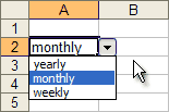 Drop Down List in Excel
You can create an in-cell drop down list in Excel by following these 4 easy steps:
- Select the cell, or range of cells, where you want to add the drop-down list.
- Go to Data > Validation > Settings tab (see image below)
- Select «List» from the Allow: drop-down box
- Enter your list in the Source: field using a comma to separate the items, or select a range of cells from your worksheet.
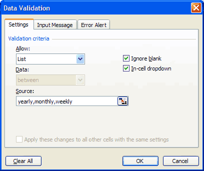 Entering the Source of a Drop Down List as a Comma-Delimited List
This approach is great for simple Yes/No options and other lists that appear only once in your spreadsheet.
The problem with this approach is that if you use this in a lot of cells and later want to update the list, you have to update all cells that use the list and there is a good chance you’ll miss one. The more elegant approach is to use a reference to a range, or even better than that — a named range.
Defining a Drop-Down List using a Range
Instead of manually entering the list of items in the data validation dialog box, you can reference a range of cells. For example, let’s say I have a separate worksheet with my list defined in cells A1:A3 as shown below. In this case, I’ve named the range «myList». You can later hide the worksheet containing your list to keep your workbook looking nice and clean or to prevent a user from changing the list.

In the data validation dialog box, instead of entering the list manually, you enter a reference to the named range in the Source field as shown below:
![]()
You could use a reference for the Source field like =Sheet2!$A$1:$A$3, but I usually prefer to name the list. Why? If you want to change the range, you only need to edit the defined name (via Formulas > Name Manager) rather than finding and editing all cells that use that particular data validation.
Note: When using a named range for a data validation list, the named range must be defined as a reference to a range of cells, or it must be a formula like OFFSET or INDIRECT or INDEX that returns a reference. If you’re thinking of getting fancy and want to define a name without a cell reference such as ={«Yes»,»No»}, the drop-down list won’t work.
Another bit of trivia: In old versions of Excel, using a named range was the only way for a drop-down list to reference a range on a different worksheet.
Check Boxes and Star Ratings with Excel Drop-Down Lists
The font used in the drop-down list cannot be changed, so it is always just a black sans serif font. This means that you can’t show different colors and fonts within the drop-down list. What I think is awesome, though, is using Unicode Character Symbols to do fun things with drop-down lists, such as star-ratings using ★ or checkboxes using the characters √, ✔, ☐, ☑ or ☒.
Important: One of the main reasons I like to use checkbox-style drop-down lists is for compatibility and ease-of-use with Excel Online and the mobile Excel apps (Form Field checkboxes don’t work in Excel Online or mobile apps). Also, when using a touch screen device, I think the drop-down checkbox is easier and more fun to use than entering an «X».
Example 1: Using a Drop Down List to create a Checkbox field
This example comes from one of my Task List templates. The Source field is just «☐,√» (without the quotes).

Example 2: Choose a Star Rating using a Drop Down Menu
For a star rating, you can use «★★★★★,★★★★,★★★,★★,★» in the Source field. This example comes from the Feature Comparison template.
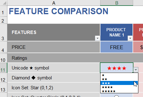
Including a Blank Value and Using Relative References
An in-cell drop down will ignore blanks if you enter text manually into the Source field (like » ,Yes,No»). So, if you want a blank value as an option, use a reference to a range as in the examples below.
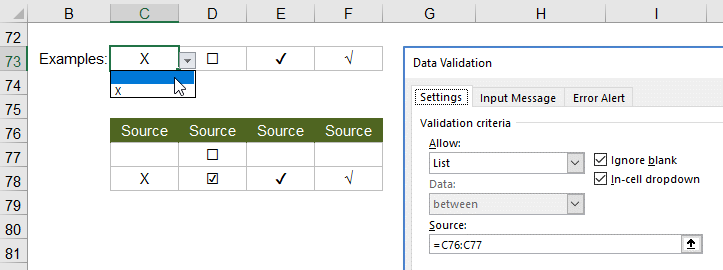
Usually, you will use absolute references like $C$76:$C$77 for the Source in your drop-down list. However, there may be times when you want the drop-down Source to change when you copy and paste the cell. In the example above, the drop-downs use a relative reference in the Source field (no $ signs in the reference). This makes it easy to create other checkbox examples by just copying the cells to the right.
Using a relative reference is important when creating dependent lists which will be shown a little later in this article.
Copying and Pasting Drop-Down Lists in Excel
When you copy and paste cells, the data validation will also be pasted, but you can’t use the Format Painter to copy and paste data validation. Instead, if you only want to copy and paste the drop-down list (and not formulas or formatting), then after copying the cell, use Paste Special and select the Validation option as shown in the image.

Customizable Drop Down Lists Using Dynamic Ranges
I like creating templates that allow a person to customize lists, such as meals for a Meal Planner or accounts for an Account Register or products for a PO with Price List.
To allow for a variable number of items within the Source range, you could use a very large range like =$A$1:$A$1000, but the drop-down would end up having a crazy amount of blanks. Instead, you can create a dynamic range that extends the list to the last value in the range.
Here is a basic example:

You can see that even though the list range $C$127:$C$133 includes two blank cells, the drop-down only extends to row 131 (the last text value in the Categories column).
Here’s how to do it:
Step 1: Create a Dynamic Named Range.
Go to Formulas > Name Manager and create a range named category_list using the following formula in the Refers To field, replacing label_cell and list_range with the appropriate cell references.
=OFFSET(label_cell,1,0,MATCH("zzzzz",list_range,1),1)
Here is the specific formula used in the example.
=OFFSET($C$127,1,0,MATCH("zzzzz",$C$127:$C$133,1)-1,1)
Step 2: Use the Named Range in the Source field for the drop-down list.
Source: =category_list
See my article «Dynamic Named Ranges» to learn more about the various formulas you can use. The formula used in the above example works well for lists that include only text values.
Dependent Drop-Down Lists Using CHOOSE or INDIRECT
A dependent drop-down list is a list that changes based on the value of another cell, which might also contain a drop-down list of its own. The Source for a drop-down list can be a formula, and that is the key to making the dependent list. As I mentioned before, the formula must return a reference, so there are only a few types of formulas that will work for drop downs. I personally prefer using CHOOSE or INDIRECT.
The example below is based on an account register where the idea is to choose categories for each transaction. The Type column contains a drop-down list that references cells C179:D179 (the labels «Expense» and «Income»). We want the dependent drop down box in the Category column to use the list of expenses if the Type is «Expense» and the list of income categories if the Type is «Income.»
Here is an example showing the CHOOSE method:
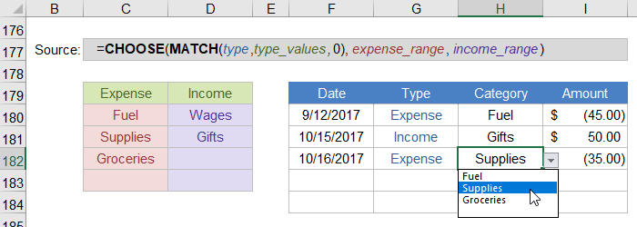
The formula uses a relative reference for the type cell and absolute references for the type_values, expense_range and income_range like this:
=CHOOSE(MATCH(G182,$C$179:$D$179,0),$C$180:$C$183,$D$180:$D$183)
Alternatively, we could create dynamic named ranges called Expense_range and Income_range and then use the following formula for the Source:
=INDIRECT(G182&"_range")
You can use named ranges within the CHOOSE formula as well, so I’m not sure whether one method is better than the other. Some may argue that CHOOSE is better because INDIRECT is a volatile function, but I don’t think that matters for drop-down lists.
See the Grocery Price Book template for a practical example of how dependent drop-down lists can be used in a spreadsheet.
Fancy Dynamic Drop-Down Lists
If the previous examples aren’t fancy enough for you, my article «Dynamic Drop-Down Lists» explains how to create drop-down lists that change based on user input, the date, check number, etc.
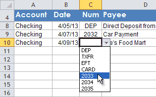
Searchable Drop-Down Lists
If your drop-down list is really long, it can be difficult to find the item you are looking for. Google Sheets provides a great solution, though not a perfect one (yet). In Sheets, you can start typing into the cell and the drop-down list will automatically filter based upon what you type … as long as it is the start of one or more of the words in the list.
For example, let’s say your list contains the names Abe Lincoln, George Washington, Harry Truman, and J. Edgar Hoover. As soon as you type «h», the list will be shortened to Harry Truman and J. Edgar Hoover, but Sheets does not recognize the «h» in Washington.
Excel: Using a fairly complicated trick, you CAN create a searchable drop-down list in Excel. See this youtube video.
More Examples
My article Add Cool Features to Your To Do Lists in Excel shows a few other examples, like using conditional formatting combined with a drop-down box to select a priority value in a to do or task list.
Example 1: This Homework To Do List allows you to choose a High, Medium, or Low value in the Priority column. There are also examples of this on the Task List template page.
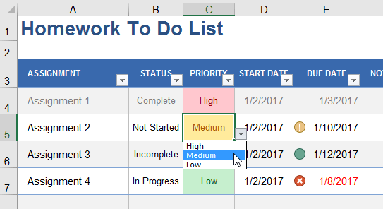
Example 2: This Task List Template uses conditional formatting icon sets for the Priority column and a drop-down list to choose a value between 1 and 4.
![]()
More Examples: Drop-down lists are a common feature in many of my templates, including the Meal Planner, Money Manager, and many financial calculators. You can download the templates to see how the drop-down lists are created.
The Customer List Template page explains how to copy a customer list worksheet into a spreadsheet, create a drop-down list showing customer names, and then add lookup formulas to display the information for the chosen customer.
Additional Resources
- Create a Drop-Down List at support.office.com — A relatively simple article and video showing how to create a drop-down list in Excel.
- Create and Manage Drop-Down Lists at support.office.com — Includes some very clear videos demonstrating the basics.
The first version of this article was originally published on 4/7/2009 at https://www.vertex42.com/ExcelTips/drop-down-list.html but the original article has been updated and integrated into this blog post.
We come across drop-down lists on the internet and other software applications all the time. They are useful because they limit the options available to the user, as only pre-validated items can be selected. In this post, we’ll look at how to add a drop-down list in Excel.
In Excel, there are three different types of worksheet-based drop-down lists:
- Data validation
- Form control
- ActiveX
So how do you know which one you should use? As with so many things, the answer is “it depends”. Let’s take a look at these three options and understand where to use each one.
Download the example file: Click the link below to download the example file used for this post:
Data validation drop-down list
The most common form of drop-down list is a data validation list. Let’s create one of these.
Enter the values to be used in the drop-down list into a range of cells; these are known as the ‘list items’.
Then select the cell in which the drop-down should exist.
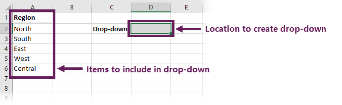
Click Data > Data Validation (drop down) > Data Validation…
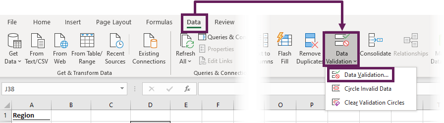
The data validation dialog box opens. On the Settings tab, select list from the allow box, and enter the range of cells containing the list in the source box.
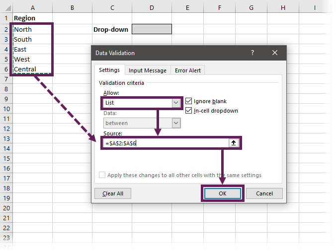
Click OK to close the data validation dialog box.
To use the drop-down, click on the cell containing the data validation list. We can now only select a value from the list.
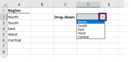
Typing an invalid entry in the cell will result in an error message.
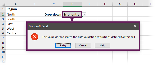
Other data validation list options
There is lots of flexibility in this type of drop-down list.
List input as hardcoded values
The list doesn’t have to be on a worksheet; the values can be hardcoded into the source field. The screenshot below shows how to include the options Yes, No and Maybe without using cells; each list item is separated by a comma
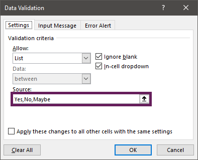
A drop-down list created in this way would look like this:
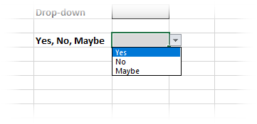
TOP TIP: If we need to use a comma in the list item text, press ALT+0130 to enter the comma, instead of a regular comma character.
List input as rows or columns
If using values in worksheet cells as the source, the list of values can be arranged in rows or columns (but not both at the same time)
List input as a named range
The list of values can be stored in a named range, provided it is a continuous range of rows or columns.
TOP TIP: If you can’t remember the name of the named range, press F3 and select from the Paste Name dialog box.
List input as a Table
I love Tables, but they don’t work as well with data validation lists as they should. Check out this post to find out how to make it work.
List input as dynamic arrays
If you have a dynamic array enabled version of Excel (only Microsoft 365 and Excel 2021), then data validation lists can contain the result of a dynamic array.
If the first cell in the output array were in cell A2, we could use =A2# as the reference in the source box. This method is excellent for advanced techniques, such as shrinking lists, or dependant lists.
Input messages
The Input Message tab of the data validation dialog box provides the settings to display a message when a user clicks the data validation cell.
The message is intended to provide guidance for the user so they know what type of information to enter.
We only need to provide a title and an input message.
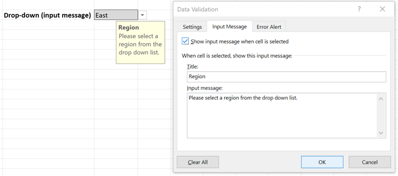
Make sure show input message when cell is selected is checked; otherwise, the message will not appear.
Error alerts
The purpose of a drop-down list of to select valid entries from a list. As a result, the chance of invalid data entry is significantly reduced. However, users can still enter text directly into the cell; therefore, invalid data entry is still possible.
The default message doesn’t provide any guidance regarding why the entry is invalid. But we can provide custom messages inside the Error Alert tab.
To provide a custom message, we only need to provide a title, an error message, and select a style icon.
Make sure show error alert after invalid data is entered is checked; otherwise, no error message will appear; a user could enter any value.
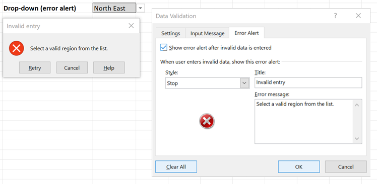
Useful notes
Before we move on, I want to make you aware of a few issues with data validation drop-down lists in Excel:
Identifying the cells containing data validation
The drop-down arrow is only visible when a user clicks on the cell. Therefore, here is no visual indicator that a cell contains a drop-down list exists until it is selected. Formatting the cell may be useful to provide a better user experience.
Copy and Paste dangers
When we copy and paste cells containing the data validation to other cells, the drop-down list is transferred as part of the format. This is great if we want to create a lot of drop-down lists containing the same items.
However… now for the danger part…
A user can copy and paste values into a cell, even if those values are not in the data validation list. If a user types into a cell, the data validation process runs; if a user pastes values into a cell, the validation is not triggered at all. This is a big problem
Here is another quirk…
If the worksheet is protected, the copy and paste overwrites the value, but retains the drop-down list. However, if the sheet is not protected, copy and paste applies the format from the source cell. As a result, the data validation drop-down list can disappear completely.
Highlight all cells with invalid options
Excel can perform a check to identify any cells containing values that do not meet the data validation criteria. Click Data > Data Validation (drop-down) > Circle Invalid Data
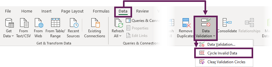
This will highlight the cells as follows:
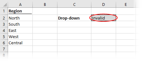
To remove the circles, click Data > Data Validation (drop-down) > Clear Validation Circles.
Form control drop-down list
Form controls can be used as another type of drop-down list in Excel. While they remove some of the negatives from data validation drop-downs, they come with their own unique challenges. VBA can be used to control form control elements; however in this post, we’ll be keeping things simple and looking at the basic non-VBA functionality (which is still pretty powerful).
Let’s start by creating a form control drop-down list. These are contained within the Developer ribbon.
Click Developer > Insert > Combo Box (Form Control)
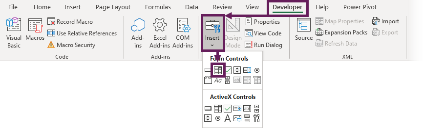
The mouse pointer will change to a cross. Click and hold the mouse while you draw the location to place the drop-down list. Holding the ALT key while placing the object will also snap the drop-down to the grid.
Right-click on the drop-down list and select format control…
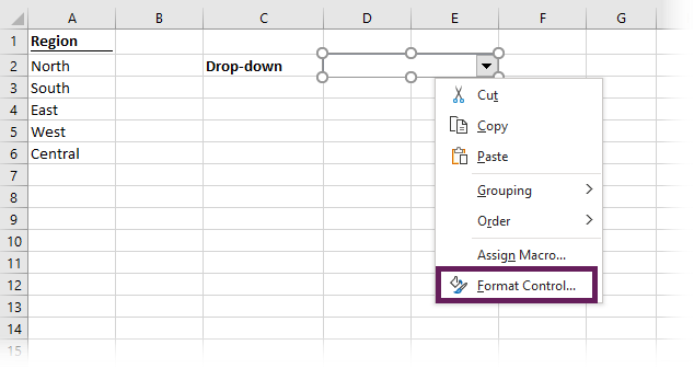
The format object window will open. Click on the control tab. The key fields are:
- Input range – the range of cells to include in the drop-down list.
- Cell link – the cell in which to output the value.
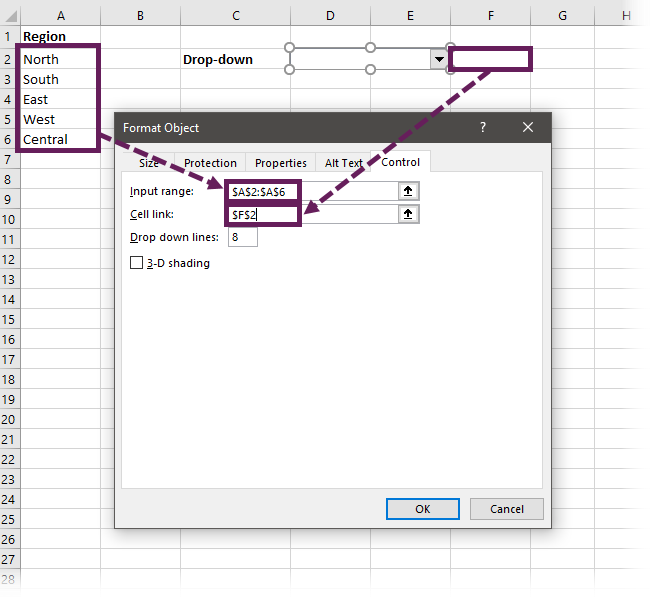
The cell selected for the cell link shows the chosen position in the drop-down box. As East is the third item in the list, cell F2 displays 3.
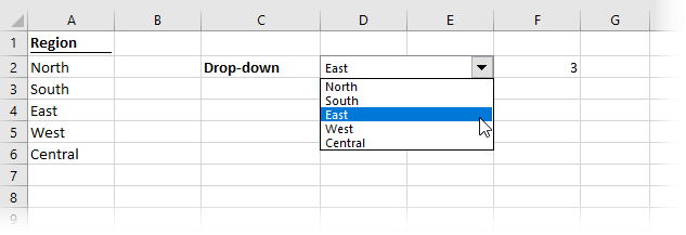
The biggest issue with the form control drop-down is that the cell link shows the position in the drop-down rather than the value itself. By using the INDEX function and the input range cells, we can retrieve the value from the list.
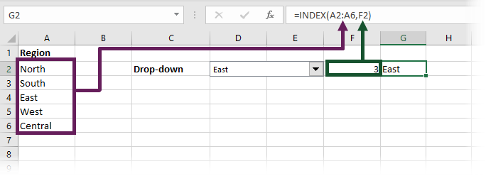
The formula in cell G2 is:
=INDEX(A2:A6,F2)
Input range options
With Form Control drop-down lists, the input range can be a standard cell range or a named range. Hardcoded lists and dynamic arrays are not compatible. However, we can use a dynamic array placed inside a named range as a workaround.
Useful notes
If we wish to have lots of drop-down lists, we can copy and paste a form control object. However, we must go into each drop-down individually to repoint to a new cell link.
We cannot enter text into the drop-down list; therefore, it is not possible to select an invalid entry.
Form controls are not compatible with Excel Online.
ActiveX drop-down list
Now for the final type of drop-down list in Excel; ActiveX drop-down list.
Click Developer > Insert > Combo Box (ActiveX Control)
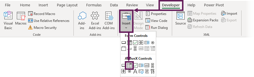
Just like the form control option shown above, draw the drop-down box on the worksheet.
Right-click on the drop-down and select properties from the menu.
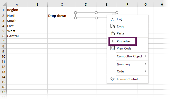
The properties dialog box opens. The critical parameters for our purposes are LinkedCell and ListFillRange. These are similar to the form control drop-down list; enter equivalent ranges into these fields. Click on the [x] in the top right corner to close the Properties window.
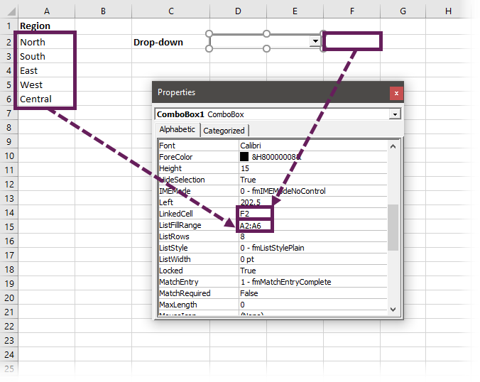
Clicking Developer > Design Mode toggles between using and editing the drop-down list. When in design mode, the drop-down can be edited, but not used. Vice versa, when in display mode, the drop-down can be used, but not edited.
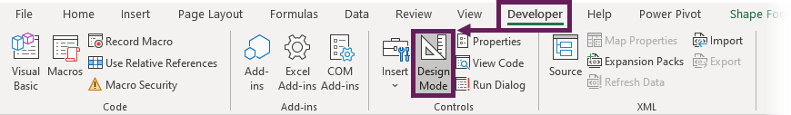
Unlike the form control version, the ActiveX drop-down displays the selected value directly in the linked cell.
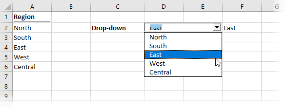
ActiveX has more extensive formatting options than form controls.
Useful notes
ActiveX drop-down boxes have many features to be aware of:
- When in design mode, the ActiveX drop-down can be copied or deleted, but not when in display mode.
- ActiveX doesn’t work on a Mac or Excel Online. So, if you want a genuinely cross-platform workbook, this is not the option for you.
Which option to choose?
So, which option should you choose for a drop-down list in Excel? As I said in the introduction, it depends. My general advice is:
- Avoid ActiveX, if possible.
- Use Form Controls for single-cell selections where strict input is required.
- Use Data Validation, where a drop-down may need to be copied.
That’s just a basic rule I use. In all cases, suitable worksheet protection needs to be applied to prevent accidental changes. Ultimately, you’ll need to experiment with all the options and work out what is best for your circumstances.

About the author
Hey, I’m Mark, and I run Excel Off The Grid.
My parents tell me that at the age of 7 I declared I was going to become a qualified accountant. I was either psychic or had no imagination, as that is exactly what happened. However, it wasn’t until I was 35 that my journey really began.
In 2015, I started a new job, for which I was regularly working after 10pm. As a result, I rarely saw my children during the week. So, I started searching for the secrets to automating Excel. I discovered that by building a small number of simple tools, I could combine them together in different ways to automate nearly all my regular tasks. This meant I could work less hours (and I got pay raises!). Today, I teach these techniques to other professionals in our training program so they too can spend less time at work (and more time with their children and doing the things they love).
Do you need help adapting this post to your needs?
I’m guessing the examples in this post don’t exactly match your situation. We all use Excel differently, so it’s impossible to write a post that will meet everybody’s needs. By taking the time to understand the techniques and principles in this post (and elsewhere on this site), you should be able to adapt it to your needs.
But, if you’re still struggling you should:
- Read other blogs, or watch YouTube videos on the same topic. You will benefit much more by discovering your own solutions.
- Ask the ‘Excel Ninja’ in your office. It’s amazing what things other people know.
- Ask a question in a forum like Mr Excel, or the Microsoft Answers Community. Remember, the people on these forums are generally giving their time for free. So take care to craft your question, make sure it’s clear and concise. List all the things you’ve tried, and provide screenshots, code segments and example workbooks.
- Use Excel Rescue, who are my consultancy partner. They help by providing solutions to smaller Excel problems.
What next?
Don’t go yet, there is plenty more to learn on Excel Off The Grid. Check out the latest posts: