For quick access to related information in another file or on a web page, you can insert a hyperlink in a worksheet cell. You can also insert links in specific chart elements.
Note: Most of the screen shots in this article were taken in Excel 2016. If you have a different version your view might be slightly different, but unless otherwise noted, the functionality is the same.
-
On a worksheet, click the cell where you want to create a link.
You can also select an object, such as a picture or an element in a chart, that you want to use to represent the link.
-
On the Insert tab, in the Links group, click Link
 .
.
You can also right-click the cell or graphic and then click Link on the shortcut menu, or you can press Ctrl+K.
-
-
Under Link to, click Create New Document.
-
In the Name of new document box, type a name for the new file.
Tip: To specify a location other than the one shown under Full path, you can type the new location preceding the name in the Name of new document box, or you can click Change to select the location that you want and then click OK.
-
Under When to edit, click Edit the new document later or Edit the new document now to specify when you want to open the new file for editing.
-
In the Text to display box, type the text that you want to use to represent the link.
-
To display helpful information when you rest the pointer on the link, click ScreenTip, type the text that you want in the ScreenTip text box, and then click OK.
 .
.-
On a worksheet, click the cell where you want to create a link.
You can also select an object, such as a picture or an element in a chart, that you want to use to represent the link.
-
On the Insert tab, in the Links group, click Link
.
You can also right-click the cell or object and then click Link on the shortcut menu, or you can press Ctrl+K.
-
-
Under Link to, click Existing File or Web Page.
-
Do one of the following:
-
To select a file, click Current Folder, and then click the file that you want to link to.
You can change the current folder by selecting a different folder in the Look in list.
-
To select a web page, click Browsed Pages and then click the web page that you want to link to.
-
To select a file that you recently used, click Recent Files, and then click the file that you want to link to.
-
To enter the name and location of a known file or web page that you want to link to, type that information in the Address box.
-
To locate a web page, click Browse the Web
, open the web page that you want to link to, and then switch back to Excel without closing your browser.
-
-
If you want to create a link to a specific location in the file or on the web page, click Bookmark, and then double-click the bookmark that you want.
Note: The file or web page that you are linking to must have a bookmark.
-
In the Text to display box, type the text that you want to use to represent the link.
-
To display helpful information when you rest the pointer on the link, click ScreenTip, type the text that you want in the ScreenTip text box, and then click OK.
 , open the web page that you want to link to, and then switch back to Excel without closing your browser.
To link to a location in the current workbook or another workbook, you can either define a name for the destination cells or use a cell reference.
-
To use a name, you must name the destination cells in the destination workbook.
How to name a cell or a range of cells
-
Select the cell, range of cells, or nonadjacent selections that you want to name.
-
Click the Name box at the left end of the formula bar
.
Name box -
In the Name box, type the name for the cells, and then press Enter.
Note: Names can’t contain spaces and must begin with a letter.
-
-
On a worksheet of the source workbook, click the cell where you want to create a link.
You can also select an object, such as a picture or an element in a chart, that you want to use to represent the link.
-
On the Insert tab, in the Links group, click Link
.
You can also right-click the cell or object and then click Link on the shortcut menu, or you can press Ctrl+K.
-
-
Under Link to, do one of the following:
-
To link to a location in your current workbook, click Place in This Document.
-
To link to a location in another workbook, click Existing File or Web Page, locate and select the workbook that you want to link to, and then click Bookmark.
-
-
Do one of the following:
-
In the Or select a place in this document box, under Cell Reference, click the worksheet that you want to link to, type the cell reference in the Type in the cell reference box, and then click OK.
-
In the list under Defined Names, click the name that represents the cells that you want to link to, and then click OK.
-
-
In the Text to display box, type the text that you want to use to represent the link.
-
To display helpful information when you rest the pointer on the link, click ScreenTip, type the text that you want in the ScreenTip text box, and then click OK.

 Name box
You can use the HYPERLINK function to create a link that opens a document that is stored on a network server, an intranet, or the Internet. When you click the cell that contains the HYPERLINK function, Excel opens the file that is stored at the location of the link.
Syntax
HYPERLINK(link_location,friendly_name)
Link_location is the path and file name to the document to be opened as text. Link_location can refer to a place in a document — such as a specific cell or named range in an Excel worksheet or workbook, or to a bookmark in a Microsoft Word document. The path can be to a file stored on a hard disk drive, or the path can be a universal naming convention (UNC) path on a server (in Microsoft Excel for Windows) or a Uniform Resource Locator (URL) path on the Internet or an intranet.
-
Link_location can be a text string enclosed in quotation marks or a cell that contains the link as a text string.
-
If the jump specified in link_location does not exist or can’t be navigated, an error appears when you click the cell.
Friendly_name is the jump text or numeric value that is displayed in the cell. Friendly_name is displayed in blue and is underlined. If friendly_name is omitted, the cell displays the link_location as the jump text.
-
Friendly_name can be a value, a text string, a name, or a cell that contains the jump text or value.
-
If friendly_name returns an error value (for example, #VALUE!), the cell displays the error instead of the jump text.
Examples
The following example opens a worksheet named Budget Report.xls that is stored on the Internet at the location named example.microsoft.com/report and displays the text «Click for report»:
=HYPERLINK(«http://example.microsoft.com/report/budget report.xls», «Click for report»)
The following example creates a link to cell F10 on the worksheet named Annual in the workbook Budget Report.xls, which is stored on the Internet at the location named example.microsoft.com/report. The cell on the worksheet that contains the link displays the contents of cell D1 as the jump text:
=HYPERLINK(«[http://example.microsoft.com/report/budget report.xls]Annual!F10», D1)
The following example creates a link to the range named DeptTotal on the worksheet named First Quarter in the workbook Budget Report.xls, which is stored on the Internet at the location named example.microsoft.com/report. The cell on the worksheet that contains the link displays the text «Click to see First Quarter Department Total»:
=HYPERLINK(«[http://example.microsoft.com/report/budget report.xls]First Quarter!DeptTotal», «Click to see First Quarter Department Total»)
To create a link to a specific location in a Microsoft Word document, you must use a bookmark to define the location you want to jump to in the document. The following example creates a link to the bookmark named QrtlyProfits in the document named Annual Report.doc located at example.microsoft.com:
=HYPERLINK(«[http://example.microsoft.com/Annual Report.doc]QrtlyProfits», «Quarterly Profit Report»)
In Excel for Windows, the following example displays the contents of cell D5 as the jump text in the cell and opens the file named 1stqtr.xls, which is stored on the server named FINANCE in the Statements share. This example uses a UNC path:
=HYPERLINK(«\FINANCEStatements1stqtr.xls», D5)
The following example opens the file 1stqtr.xls in Excel for Windows that is stored in a directory named Finance on drive D, and displays the numeric value stored in cell H10:
=HYPERLINK(«D:FINANCE1stqtr.xls», H10)
In Excel for Windows, the following example creates a link to the area named Totals in another (external) workbook, Mybook.xls:
=HYPERLINK(«[C:My DocumentsMybook.xls]Totals»)
In Microsoft Excel for the Macintosh, the following example displays «Click here» in the cell and opens the file named First Quarter that is stored in a folder named Budget Reports on the hard drive named Macintosh HD:
=HYPERLINK(«Macintosh HD:Budget Reports:First Quarter», «Click here»)
You can create links within a worksheet to jump from one cell to another cell. For example, if the active worksheet is the sheet named June in the workbook named Budget, the following formula creates a link to cell E56. The link text itself is the value in cell E56.
=HYPERLINK(«[Budget]June!E56», E56)
To jump to a different sheet in the same workbook, change the name of the sheet in the link. In the previous example, to create a link to cell E56 on the September sheet, change the word «June» to «September.»
When you click a link to an email address, your email program automatically starts and creates an email message with the correct address in the To box, provided that you have an email program installed.
-
On a worksheet, click the cell where you want to create a link.
You can also select an object, such as a picture or an element in a chart, that you want to use to represent the link.
-
On the Insert tab, in the Links group, click Link
.
You can also right-click the cell or object and then click Link on the shortcut menu, or you can press Ctrl+K.
-
-
Under Link to, click E-mail Address.
-
In the E-mail address box, type the email address that you want.
-
In the Subject box, type the subject of the email message.
Note: Some web browsers and email programs may not recognize the subject line.
-
In the Text to display box, type the text that you want to use to represent the link.
-
To display helpful information when you rest the pointer on the link, click ScreenTip, type the text that you want in the ScreenTip text box, and then click OK.
You can also create a link to an email address in a cell by typing the address directly in the cell. For example, a link is created automatically when you type an email address, such as someone@example.com.
You can insert one or more external reference (also called links) from a workbook to another workbook that is located on your intranet or on the Internet. The workbook must not be saved as an HTML file.
-
Open the source workbook and select the cell or cell range that you want to copy.
-
On the Home tab, in the Clipboard group, click Copy.
-
Switch to the worksheet that you want to place the information in, and then click the cell where you want the information to appear.
-
On the Home tab, in the Clipboard group, click Paste Special.
-
Click Paste Link.
Excel creates an external reference link for the cell or each cell in the cell range.

Note: You may find it more convenient to create an external reference link without opening the workbook on the web. For each cell in the destination workbook where you want the external reference link, click the cell, and then type an equal sign (=), the URL address, and the location in the workbook. For example:
=’http://www.someones.homepage/[file.xls]Sheet1′!A1
=’ftp.server.somewhere/file.xls’!MyNamedCell
To select a hyperlink without activating the link to its destination, do one of the following:
-
Click the cell that contains the link, hold the mouse button until the pointer becomes a cross
, and then release the mouse button. -
Use the arrow keys to select the cell that contains the link.
-
If the link is represented by a graphic, hold down Ctrl, and then click the graphic.
You can change an existing link in your workbook by changing its destination, its appearance, or the text or graphic that is used to represent it.
Change the destination of a link
-
Select the cell or graphic that contains the link that you want to change.
Tip: To select a cell that contains a link without going to the link destination, click the cell and hold the mouse button until the pointer becomes a cross
, and then release the mouse button. You can also use the arrow keys to select the cell. To select a graphic, hold down Ctrl and click the graphic.-
On the Insert tab, in the Links group, click Link.
You can also right-click the cell or graphic and then click Edit Link on the shortcut menu, or you can press Ctrl+K.
-
-
In the Edit Hyperlink dialog box, make the changes that you want.
Note: If the link was created by using the HYPERLINK worksheet function, you must edit the formula to change the destination. Select the cell that contains the link, and then click the formula bar to edit the formula.
You can change the appearance of all link text in the current workbook by changing the cell style for links.
-
On the Home tab, in the Styles group, click Cell Styles.
-
Under Data and Model, do the following:
-
To change the appearance of links that have not been clicked to go to their destinations, right-click Link, and then click Modify.
-
To change the appearance of links that have been clicked to go to their destinations, right-click Followed Link, and then click Modify.
Note: The Link cell style is available only when the workbook contains a link. The Followed Link cell style is available only when the workbook contains a link that has been clicked.
-
-
In the Style dialog box, click Format.
-
On the Font tab and Fill tab, select the formatting options that you want, and then click OK.
Notes:
-
The options that you select in the Format Cells dialog box appear as selected under Style includes in the Style dialog box. You can clear the check boxes for any options that you don’t want to apply.
-
Changes that you make to the Link and Followed Link cell styles apply to all links in the current workbook. You can’t change the appearance of individual links.
-
-
Select the cell or graphic that contains the link that you want to change.
Tip: To select a cell that contains a link without going to the link destination, click the cell and hold the mouse button until the pointer becomes a cross
, and then release the mouse button. You can also use the arrow keys to select the cell. To select a graphic, hold down Ctrl and click the graphic. -
Do one or more of the following:
-
To change the link text, click in the formula bar, and then edit the text.
-
To change the format of a graphic, right-click it, and then click the option that you need to change its format.
-
To change text in a graphic, double-click the selected graphic, and then make the changes that you want.
-
To change the graphic that represents the link, insert a new graphic, make it a link with the same destination, and then delete the old graphic and link.
-
-
Right-click the hyperlink that you want to copy or move, and then click Copy or Cut on the shortcut menu.
-
Right-click the cell that you want to copy or move the link to, and then click Paste on the shortcut menu.
By default, unspecified paths to hyperlink destination files are relative to the location of the active workbook. Use this procedure when you want to set a different default path. Each time that you create a link to a file in that location, you only have to specify the file name, not the path, in the Insert Hyperlink dialog box.
Follow one of the steps depending on the Excel version you are using:
-
In Excel 2016, Excel 2013, and Excel 2010:
-
Click the File tab.
-
Click Info.
-
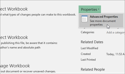
Click Properties, and then select Advanced Properties.
-
In the Summary tab, in the Hyperlink base text box, type the path that you want to use.
Note: You can override the link base address by using the full, or absolute, address for the link in the Insert Hyperlink dialog box.
-
-
In Excel 2007:
-
Click the Microsoft Office Button
, click Prepare, and then click Properties. -
In the Document Information Panel, click Properties, and then click Advanced Properties.
-
Click the Summary tab.
-
In the Hyperlink base box, type the path that you want to use.
Note: You can override the link base address by using the full, or absolute, address for the link in the Insert Hyperlink dialog box.
-
 , click Prepare, and then click Properties.
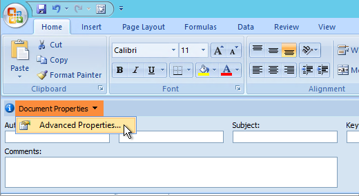
To delete a link, do one of the following:
-
To delete a link and the text that represents it, right-click the cell that contains the link, and then click Clear Contents on the shortcut menu.
-
To delete a link and the graphic that represents it, hold down Ctrl and click the graphic, and then press Delete.
-
To turn off a single link, right-click the link, and then click Remove Link on the shortcut menu.
-
To turn off several links at once, do the following:
-
In a blank cell, type the number 1.
-
Right-click the cell, and then click Copy on the shortcut menu.
-
Hold down Ctrl and select each link that you want to turn off.
Tip: To select a cell that has a link in it without going to the link destination, click the cell and hold the mouse button until the pointer becomes a cross
, and then release the mouse button. -
On the Home tab, in the Clipboard group, click the arrow below Paste, and then click Paste Special.
-
Under Operation, click Multiply, and then click OK.
-
On the Home tab, in the Styles group, click Cell Styles.
-
Under Good, Bad, and Neutral, select Normal.
-
A link opens another page or file when you click it. The destination is frequently another web page, but it can also be a picture, or an email address, or a program. The link itself can be text or a picture.
When a site user clicks the link, the destination is shown in a Web browser, opened, or run, depending on the type of destination. For example, a link to a page shows the page in the web browser, and a link to an AVI file opens the file in a media player.
How links are used
You can use links to do the following:
-
Navigate to a file or web page on a network, intranet, or Internet
-
Navigate to a file or web page that you plan to create in the future
-
Send an email message
-
Start a file transfer, such as downloading or an FTP process
When you point to text or a picture that contains a link, the pointer becomes a hand  , indicating that the text or picture is something that you can click.
What a URL is and how it works
When you create a link, its destination is encoded as a Uniform Resource Locator (URL), such as:
http://example.microsoft.com/news.htm
file://ComputerName/SharedFolder/FileName.htm
A URL contains a protocol, such as HTTP, FTP, or FILE, a Web server or network location, and a path and file name. The following illustration defines the parts of the URL:
1. Protocol used (http, ftp, file)
2. Web server or network location
3. Path
4. File name
Absolute and relative links
An absolute URL contains a full address, including the protocol, the Web server, and the path and file name.
A relative URL has one or more missing parts. The missing information is taken from the page that contains the URL. For example, if the protocol and web server are missing, the web browser uses the protocol and domain, such as .com, .org, or .edu, of the current page.
It is common for pages on the web to use relative URLs that contain only a partial path and file name. If the files are moved to another server, any links will continue to work as long as the relative positions of the pages remain unchanged. For example, a link on Products.htm points to a page named apple.htm in a folder named Food; if both pages are moved to a folder named Food on a different server, the URL in the link will still be correct.
In an Excel workbook, unspecified paths to link destination files are by default relative to the location of the active workbook. You can set a different base address to use by default so that each time that you create a link to a file in that location, you only have to specify the file name, not the path, in the Insert Hyperlink dialog box.
-
On a worksheet, select the cell where you want to create a link.
-
On the Insert tab, select Hyperlink.
You can also right-click the cell and then select Hyperlink… on the shortcut menu, or you can press Ctrl+K.
-
Under Display Text:, type the text that you want to use to represent the link.
-
Under URL:, type the complete Uniform Resource Locator (URL) of the webpage you want to link to.
-
Select OK.
To link to a location in the current workbook, you can either define a name for the destination cells or use a cell reference.
-
To use a name, you must name the destination cells in the workbook.
How to define a name for a cell or a range of cells
Note: In Excel for the Web, you can’t create named ranges. You can only select an existing named range from the Named Ranges control. Alternately, you can open the file in the Excel desktop app, create a named range there, and then access this option from Excel for the web.
-
Select the cell or range of cells that you want to name.
-
On the Name Box box at the left end of the formula bar
, type the name for the cells, and then press Enter.Note: Names can’t contain spaces and must begin with a letter.
-
-
On the worksheet, select the cell where you want to create a link.
-
On the Insert tab, select Hyperlink.
You can also right-click the cell and then select Hyperlink… on the shortcut menu, or you can press Ctrl+K.
-
Under Display Text:, type the text that you want to use to represent the link.
-
Under Place in this document:, enter the defined name or cell reference.
-
Select OK.
When you click a link to an email address, your email program automatically starts and creates an email message with the correct address in the To box, provided that you have an email program installed.
-
On a worksheet, select the cell where you want to create a link.
-
On the Insert tab, select Hyperlink.
You can also right-click the cell and then select Hyperlink… on the shortcut menu, or you can press Ctrl+K.
-
Under Display Text:, type the text that you want to use to represent the link.
-
Under E-mail address:, type the email address that you want.
-
Select OK.
You can also create a link to an email address in a cell by typing the address directly in the cell. For example, a link is created automatically when you type an email address, such as someone@example.com.
You can use the HYPERLINK function to create a link to a URL.
Note: The Link_location can be a text string enclosed in quotation marks or a reference to a cell that contains the link as a text string.
To select a hyperlink without activating the link to its destination, do any of the following:
-
Select a cell by clicking it when the pointer is an arrow.
-
Use the arrow keys to select the cell that contains the link.
You can change an existing link in your workbook by changing its destination, its appearance, or the text that is used to represent it.
-
Select the cell that contains the link that you want to change.
Tip: To select a hyperlink without activating the link to its destination, use the arrow keys to select the cell that contains the link.
-
On the Insert tab, select Hyperlink.
You can also right-click the cell or graphic and then select Edit Hyperlink… on the shortcut menu, or you can press Ctrl+K.
-
In the Edit Hyperlink dialog box, make the changes that you want.
Note: If the link was created by using the HYPERLINK worksheet function, you must edit the formula to change the destination. Select the cell that contains the link, and then select the formula bar to edit the formula.
-
Right-click the hyperlink that you want to copy or move, and then select Copy or Cut on the shortcut menu.
-
Right-click the cell that you want to copy or move the link to, and then select Paste on the shortcut menu.
To delete a link, do one of the following:
-
To delete a link, select the cell and press Delete.
-
To turn off a link (delete the link but keep the text that represents it), right-click the cell and then select Remove Hyperlink.
Need more help?
You can always ask an expert in the Excel Tech Community or get support in the Answers community.
See Also
Remove or turn off links
Working with Excel, a day will come when you’ll need to reference data from one workbook in another one. It’s a common use case and pretty easy to pull off. Join us as we explain how to link two Excel files and discuss many possible scenarios.
How to link Excel files – what are the available options?
Just as there are many different versions of Excel, the ways to link data also differ. It’s a lot easier if you share your Excel files in OneDrive rather than locally but we’ll discuss both scenarios.
Choosing how to link data depends also on the sheer volume of what you wish to link. If we’re talking here about particular cells or a column from your workbook, the default methods will do just fine. If you’re after linking entire Excel files, using tools such as Coupler.io with its Excel integrations may prove to be more efficient. But we’ll get to that!
You can link two or more Excel files stored on your hard drive. When the data changes in a Source file, the change will be quickly reflected in the Destination file.
The drawback of this approach is that it will only work on your local machine. Even if you share both files with another user, the link will cease to exist and they’ll be forced to re-add it. What’s more, the data will be only updated if both files are open at the same time.
So if you have a choice, it’s better to add both files to your OneDrive. If they’re already in there, you may as well jump to the How to link between Cloud-based Excel files section.
To link 2 Excel files stored locally, you have two options:
- Type in a formula referencing the exact location in a Source file
- Copy the desired cells and paste them as a link
How to link between files in desktop Excel?
To reference a single cell in another local file, you’ll use the following formula:
=[SourceWorkbook.xlsx]Sheet1!$A$1
Replace SourceWorkbook.xlsx with the name of the file stored on your machine. Then, point to an exact sheet and a cell. A reference to a range of cells could like this:
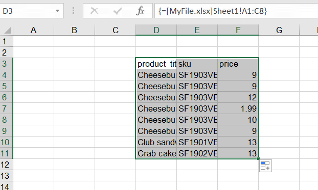
=[MyFile.xlsx]Sheet1!A1:C8
Press ENTER to save the formula and pull the data. If you’re on an older version of Excel, you may need to press CTRL+SHIFT+ENTER instead.
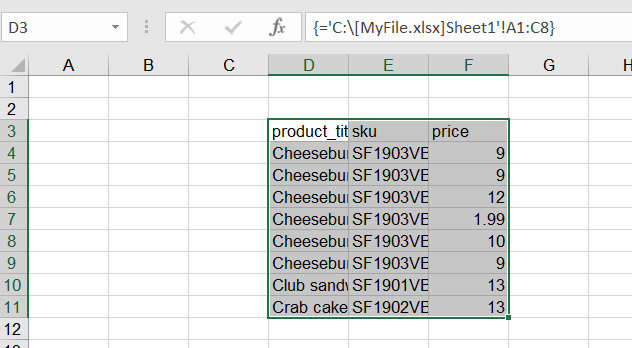
When you close the Source file, the formulas will change to include the entire path of the file – for example:
='C:[MyFile.xlsx]Sheet1'!A1:C8
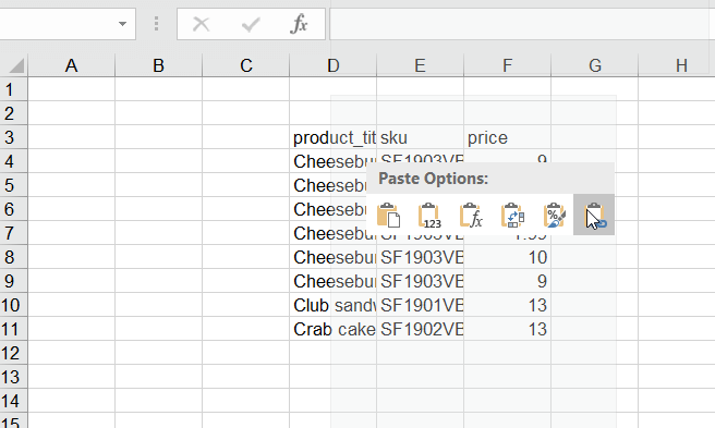
As an alternative, you can:
- Open a Source file, select the desired cells, and copy them.

- Head back to the Destination file, right-click on a desired cell or cells and choose to paste as a link.

- Here is the result:
Note that if the Source file is closed, and you reference it with a formula, no data will be pulled until you open a file.
How to link between cloud-based files in Excel?
When you wish to link Excel Online files or use those stored in OneDrive, things become easier. You can freely share files among coworkers and any interlinking won’t be affected. Links in files also refresh in near real time, giving you peace of mind that you’re working with the latest data.
The feature that enables it is called Workbook Links. We’ll explain how it works in the following chapters.
Workbook Links are suitable for individual cells or ranges of them. You may also link individual columns but the more data is involved, the slower your calculations will be. If you’re going to be linking entire worksheets or workbooks, it’s far better to focus on importing, rather than linking them. This is best done with dedicated tools.
There is more on that in the How to link a wide range of cells to Excel or another service chapter.
How to link two Excel files?
Let’s start with a most basic use case – you’re running some operations in your Excel workbook. In one of the fields, you wish to use the value(s) from another workbook and have it update automatically.
The flow is simple:
- In workbook 1 (source), highlight the data you want to link and copy it.
- In workbook 2 (destination), right-click on the first row and select the Link icon.

The latest data will be imported. A yellow bar will, however, appear now as well as every time you open a destination workbook.

To enable the data sync, select Enable Content.
For some more advanced settings, you can choose the Manage Workbook Links button to look up the list of connected workbooks and a status for each – most likely it will be Connection Blocked.
To sync, press the Enable Content button from the yellow bar.

If any errors occur, you’ll see them in the menu to the right. For each of the connected files, you can press the Refresh button to manually pull the latest data. You can also use the button above to refresh data for all your links.
Of course, the whole idea of creating links between workbooks is not to keep refreshing the data manually. Once the data has been refreshed, an option to set automatic updates will be enabled.
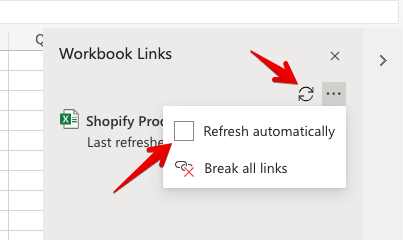
If you tick Refresh automatically, the data will start to refresh periodically.
How to link a wide range of cells to Excel or another service?
The more data you link, the more computing your Excel needs to perform to pull the data and refresh it. It’s not an issue if you have a few or a few dozens of links spread across files.
However, if you wish to regularly pull thousands of cells into your workbooks, it will significantly slow down your workbooks. It may delay the data refresh and may leave you wondering whether the data has already been refreshed or not.
To avoid that, for larger operations it’s better to use tools dedicated to importing data such as Coupler.io. With Coupler.io, you can pull the desired ranges of cells directly into another Excel workbook or worksheet. You can then refresh the data automatically at a chosen schedule.
If you wish to, you can also import the Excel data to other services, such as Google Sheets or Google BigQuery, or bring it to Excel from Airtable, Pipedrive, Hubspot, and many others.
To get started with Coupler.io, create an account, log in, and click the Add an importer button.
From the list of source applications, choose Excel.

Next, click the Connect button. Log in with your Microsoft account and allow for Coupler.io to connect.
Once connected, you’ll need to choose the workbook from your OneDrive that we’ll be importing from. Also select the worksheet in this file.
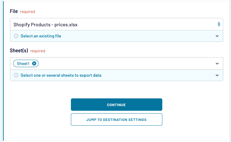
Although it’s optional, most often you’ll want to specify the range of cells to import. If you don’t, all data from a given sheet will be fetched.
You may use the standard Excel formatting and pull, for example, cells C1:D8. You may also pull an entire column by typing, for example, C1:C.

Jumping to the Destination settings, choose where to import the data to. We’ll go with Excel as we just want to move the data from one workbook to another but there are other options available too.
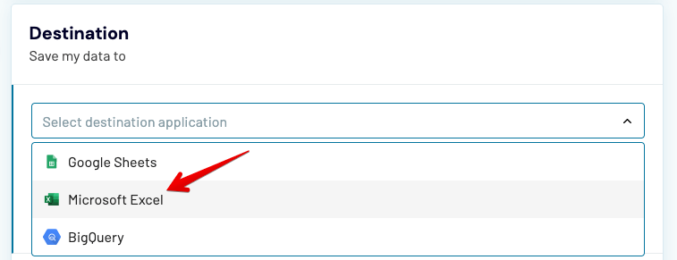
If you’re importing from Excel to Excel, there’s no need to connect your account again, unless you’re importing to someone else’s account. Select it, and specify the exact destination.
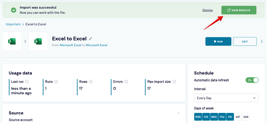
Finally, you can create a schedule for when the data should be imported. Choose what works best for you and run the importer.

Give it a little while to load, and then open the destination worksheet to see the results.
How to link Excel files and sync in real-time?
One of the advantages of using Excel files stored on OneDrive is their ability to sync data between one another. Microsoft advertises it as real-time sync but after some tests, we would call it a near real time.
If you’re used to the refresh rate of Google Sheets, for example, you may be disappointed. However, in most situations, a slight delay won’t cause any trouble.
To link files in Excel, follow the steps we outlined in the How to link Excel files chapter.
When data is changed in the destination file, most likely you won’t see an update visible right away in the source file. If you do nothing about it and just move on to the next task, you should see a refreshed number in a cell in a few minutes’ time. It will then continue refreshing at regular intervals.
If you want to speed things up, you can run an instant refresh by clicking Data -> Workbook Links in the menu and then the icon to refresh the data from a particular workbook.

This will often work, but only if the data in the source workbook has already been saved. Once again, it doesn’t happen instantly but only at regular (quite frequent) intervals.
If you’re anxious to have the data refreshed presently, you may consider refreshing the source file after making a change. This will prompt an automatic save. After that, manually force a data refresh in the destination file and it will fetch the latest saved data.
As a reminder, if you use Coupler.io to import data from one Excel workbook to another, you decide on the refresh schedule. For some, morning sync from Monday to Friday will do just fine. Others will prefer more frequent syncs – with Coupler.io you can even do it every 15 minutes.
FAQ: How to link Excel files
Let’s now discuss some specific use cases for how to link files in Excel. The tips below apply for files stored in OneDrive. If you only use Excel locally, jump back to the How to link local files in Excel section.
How to link cells in different Excel files?
For linking individual cells across files, the procedure is very much the same as we discussed earlier:
- Highlight the cell you want to reuse elsewhere and copy it.
- Right-click on the desired destination and select the Link icon from the Paste Options section.
If you’re importing to the same workbook as before, you won’t need to Enable Content again. If you reloaded it in the meantime, or are just linking the data to a new workbook, choose Manage Workbook Links and then Enable Content from the same bar.
Note that if you link multiple sets of cells or data ranges from the same workbook serving as a Source, they will all appear as a single position on your list of Workbook Links.
In the example below, you can see the data we imported from our sample Shopify store using Coupler.io.
We have a range of prices to the left linked from the respective workbook. Below there’s also a name of one of our products linked from another place in the same workbook. To the right, we can refresh data for all linked fields or, for example, enable automatic data refreshes.

How to link two Excel files without opening the source file?
You can link files in Excel without actually opening the source file. Of course, you’ll need to know the exact location of the cell or range of cells you wish to link. What’s more, to link Excel Online files or anything else stored on your OneDrive, you’ll need to fetch your unique ID.
To do so, set up a link in the traditional way we described above. Then, click on any linked cell in the Destination file and check its formula. It will look something like this:
='https://d.docs.live.net/18644c626caae38c/[myworkbook1.xlsx]Sheet1'!$C$2
The ID will follow right after the live.net link:

To insert a link from any given workbook, copy the formula with your ID and swap the file name and the cell range with the right values. Press ENTER and the latest data will be fetched.
How to link Excel columns between files?
Choosing a range of cells limits you to only the values currently present in the Source workbook. If anything new appears, it won’t be linked and, as such, won’t appear in the Destination workbook.
The solution is often to link an entire column and reference it in another file. To do so, click on any column in the Source file and copy it.
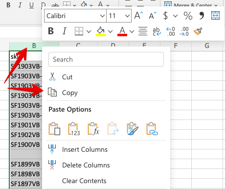
Then, select the first row of a column you want to add a link to and choose the Link icon. All the rows from the chosen column will be imported.

Rather than click, you can also enter the formulas directly. To link an entire column, it’s best to link to the first cell and then stretch the formula to the other rows.
When you insert the formula for the first row, be sure to remove the second $ (dollar) sign pointing to the specific cell. So, instead of the reference:
(...)Sheet1'!$C$2
Make it:
(...)Sheet1'!$C2
How to link fields between multiple files in Excel?
Advanced calculations may require referencing data from multiple spreadsheets at the same time. In the same way, the calculated data can then be referenced in other workbooks, creating a complex network of interconnected links.
As you recall from the earlier chapters, the formulas for linking cells between Excel Online files look somewhat like this:
='https://d.docs.live.net/18373e637ca3e48c/[Shopify Products - prices.xlsx]Sheet1'!$C$8
For the purpose of running any calculations or just adjusting the formulas as we go, the link is far too complex. It’s much better to link the desired fields into the destination workbook and then reference them from another worksheet in the same workbook.
To do so, create a separate worksheet in your destination file where you’ll link all the external data. Name it accordingly – for example, “Sources”. Link the desired data by copying it from the source file and then pasting it as links (just as we did before).
Then, jump to the worksheet in the destination file. To reference the data from another sheet, use the following pattern:
Sheet_name!$A$1
For example, for calculating the average value of a range of cells present now in another worksheet, we would use:
=AVERAGE(Sources!B2:B12)
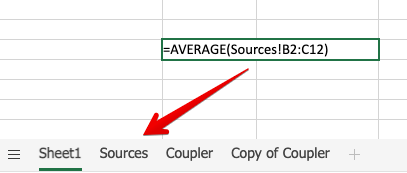
You can also type in the “=” sign (plus optionally a function name) and then jump to another worksheet and highlight the arguments. Press ENTER and the formula will be resolved.
In the standard version of Excel, the approach is pretty much the same, just with some small changes in the syntax of the links, as we mentioned earlier.
How to link Excel files – summing up
Linking Excel files can save you plenty of time and help you automate many dull processes.
It can also make things harder if you begin to link from one file to another, then to another, and another. The more interconnected workbooks become, the more complex it will be to troubleshoot the entire flow.
Find the right balance and use the right methods for linking your data.
When moving individual cells or ranges of them, Workbook Links work perfectly and are very easy to set up.
For moving large sets of data between workbooks or linking entire files, it’s a lot better to use tools such as Coupler.io. You’ll be able to set up your own schedule for imports, and all data transfers will happen outside of Excel. As a result, no Excel resources will be used, and you’ll be able to work much more smoothly while the information is synced in the background.
Thanks for reading!
-

Technical Content Writer on Coupler.io who loves working with data, writing about it, and even producing videos about it. I’ve worked at startups and product companies, writing content for technical audiences of all sorts. You’ll often see me cycling🚴🏼♂️, backpacking around the world🌎, and playing heavy board games.

Back to Blog
Focus on your business
goals while we take care of your data!
Try Coupler.io
Содержание
- Insert an object in your Excel spreadsheet
- Find links (external references) in a workbook
- Find links used in formulas
- Need more help?
- HYPERLINK function
- Description
- Syntax
- Remark
- Examples
- How to find and remove external links in Excel
- How to find cells with external links in Excel
- How to find links in Excel named ranges (defined names)
- How to identify external links in Excel objects
- How to find links to other files in Excel charts
- How to find external links in Pivot Tables
- How to enable links to external workbooks in Excel
- Control the security prompt about updating links
- Change security setting for external links
- How to break external links in Excel
- Get a list of all external links in a workbook
- Traditional approach
- Dynamic arrays and Excel 4.0 macros.
- Step 1. Create a new name that references the macro
- Step 2. Use the newly create name in a formula
- VBA macro to get a list of external links
- Find cells with external links using VBA
- Find all external links in a workbook in a click
Insert an object in your Excel spreadsheet
You can use Object Linking and Embedding (OLE) to include content from other programs, such as Word or Excel.
OLE is supported by many different programs, and OLE is used to make content that is created in one program available in another program. For example, you can insert an Office Word document in an Office Excel workbook. To see what types of content that you can insert, click Object in the Text group on the Insert tab. Only programs that are installed on your computer and that support OLE objects appear in the Object type box.
If you copy information between Excel or any program that supports OLE, such as Word, you can copy the information as either a linked object or an embedded object. The main differences between linked objects and embedded objects are where the data is stored and how the object is updated after you place it in the destination file. Embedded objects are stored in the workbook that they are inserted in, and they are not updated. Linked objects remain as separate files, and they can be updated.
Linked and embedded objects in a document
1. An embedded object has no connection to the source file.
2. A linked object is linked to the source file.
3. The source file updates the linked object.
When to use linked objects
If you want the information in your destination file to be updated when the data in the source file changes, use linked objects.
With a linked object, the original information remains stored in the source file. The destination file displays a representation of the linked information but stores only the location of the original data (and the size if the object is an Excel chart object). The source file must remain available on your computer or network to maintain the link to the original data.
The linked information can be updated automatically if you change the original data in the source file. For example, if you select a paragraph in a Word document and then paste the paragraph as a linked object in an Excel workbook, the information can be updated in Excel if you change the information in your Word document.
When to use embedded objects
If you don’t want to update the copied data when it changes in the source file, use an embedded object. The version of the source is embedded entirely in the workbook. If you copy information as an embedded object, the destination file requires more disk space than if you link the information.
When a user opens the file on another computer, he can view the embedded object without having access to the original data. Because an embedded object has no links to the source file, the object is not updated if you change the original data. To change an embedded object, double-click the object to open and edit it in the source program. The source program (or another program capable of editing the object) must be installed on your computer.
Changing the way that an OLE object is displayed
You can display a linked object or embedded object in a workbook exactly as it appears in the source program or as an icon. If the workbook will be viewed online, and you don’t intend to print the workbook, you can display the object as an icon. This minimizes the amount of display space that the object occupies. Viewers who want to display the information can double-click the icon.
Источник
Find links (external references) in a workbook
Linking to other workbooks is a very common task in Excel, but sometimes you might find yourself with a workbook that has links you can’t find even though Excel tells you they exist. There is no automatic way to find all external references that are used in a workbook, however, there are several manual methods you can use to find them. You need to look in formulas, defined names, objects (like text boxes or shapes), chart titles, and chart data series.
Any Excel workbook you’ve linked to will have that workbook’s filename in the link with its .xl* file extension (like .xls, .xlsx, .xlsm), so a recommended method is to look for all references to the .xl partial file extension. If you’re linking to another source, you’ll need to determine the best search term to use.
Find links used in formulas
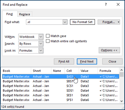
Press Ctrl+F to launch the Find and Replace dialog.
In the Find what box, enter .xl.
In the Within box, click Workbook.
In the Look in box, click Formulas.
In the list box that is displayed, look in the Formula column for formulas that contain .xl. In this case, Excel found multiple instances of Budget Master.xlsx.
To select the cell with an external reference, click the cell address link for that row in the list box.
Tip: Click any column header to sort the column, and group all of the external references together.
On the Formulas tab, in the Defined Names group, click Name Manager.
Check each entry in the list, and look in the Refers To column for external references. External references contain a reference to another workbook, such as [Budget.xlsx].
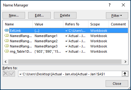
Click any column header to sort the column, and group all of the external references together.
You can group multiple items with the Shift or Ctrl keys and Left-click if you want to delete multiple items at once.
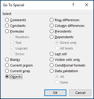
Press Ctrl+G, the shortcut for the Go To dialog, then click Special > Objects > OK. This will select all objects on the active worksheet.
 Special dialog» loading=»lazy»>
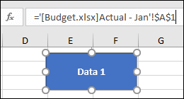
Press the Tab key to move between each of the selected objects, and then look in the formula bar  for a reference to another workbook, such as [Budget.xlsx].
Click the chart title on the chart that you want to check.
In the formula bar , look for a reference to another workbook, such as [Budget.xls].
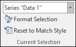
Select the chart that you want to check.
On the Layout tab, in the Current Selection group, click the arrow next to the Chart Elements box, and then click the data series that you want to check.
 Format > Current Selection» loading=»lazy»>
In the formula bar , look for a reference to another workbook, such as [Budget.xls] in the SERIES function.
Need more help?
You can always ask an expert in the Excel Tech Community or get support in the Answers community.
Источник
HYPERLINK function
This article describes the formula syntax and usage of the HYPERLINK function in Microsoft Excel.
Description
The HYPERLINK function creates a shortcut that jumps to another location in the current workbook, or opens a document stored on a network server, an intranet, or the Internet. When you click a cell that contains a HYPERLINK function, Excel jumps to the location listed, or opens the document you specified.
Syntax
The HYPERLINK function syntax has the following arguments:
Link_location Required. The path and file name to the document to be opened. Link_location can refer to a place in a document — such as a specific cell or named range in an Excel worksheet or workbook, or to a bookmark in a Microsoft Word document. The path can be to a file that is stored on a hard disk drive. The path can also be a universal naming convention (UNC) path on a server (in Microsoft Excel for Windows) or a Uniform Resource Locator (URL) path on the Internet or an intranet.
Note Excel for the web the HYPERLINK function is valid for web addresses (URLs) only. Link_location can be a text string enclosed in quotation marks or a reference to a cell that contains the link as a text string.
If the jump specified in link_location does not exist or cannot be navigated, an error appears when you click the cell.
Friendly_name Optional. The jump text or numeric value that is displayed in the cell. Friendly_name is displayed in blue and is underlined. If friendly_name is omitted, the cell displays the link_location as the jump text.
Friendly_name can be a value, a text string, a name, or a cell that contains the jump text or value.
If friendly_name returns an error value (for example, #VALUE!), the cell displays the error instead of the jump text.
In the Excel desktop application, to select a cell that contains a hyperlink without jumping to the hyperlink destination, click the cell and hold the mouse button until the pointer becomes a cross  , then release the mouse button. In Excel for the web, select a cell by clicking it when the pointer is an arrow; jump to the hyperlink destination by clicking when the pointer is a pointing hand.
Examples
=HYPERLINK(«http://example.microsoft.com/report/budget report.xlsx», «Click for report»)
Opens a workbook saved at http://example.microsoft.com/report. The cell displays «Click for report» as its jump text.
=HYPERLINK(«[http://example.microsoft.com/report/budget report.xlsx]Annual!F10», D1)
Creates a hyperlink to cell F10 on the Annual worksheet in the workbook saved at http://example.microsoft.com/report. The cell on the worksheet that contains the hyperlink displays the contents of cell D1 as its jump text.
=HYPERLINK(«[http://example.microsoft.com/report/budget report.xlsx]’First Quarter’!DeptTotal», «Click to see First Quarter Department Total»)
Creates a hyperlink to the range named DeptTotal on the First Quarter worksheet in the workbook saved at http://example.microsoft.com/report. The cell on the worksheet that contains the hyperlink displays «Click to see First Quarter Department Total» as its jump text.
=HYPERLINK(«http://example.microsoft.com/Annual Report.docx]QrtlyProfits», «Quarterly Profit Report»)
To create a hyperlink to a specific location in a Word file, you use a bookmark to define the location you want to jump to in the file. This example creates a hyperlink to the bookmark QrtlyProfits in the file Annual Report.doc saved at http://example.microsoft.com.
Displays the contents of cell D5 as the jump text in the cell and opens the workbook saved on the FINANCE server in the Statements share. This example uses a UNC path.
Opens the workbook 1stqtr.xlsx that is stored in the Finance directory on drive D, and displays the numeric value that is stored in cell H10.
Creates a hyperlink to the Totals area in another (external) workbook, Mybook.xlsx.
=HYPERLINK(«[Book1.xlsx]Sheet1!A10″,»Go to Sheet1 > A10»)
To jump to a different location in the current worksheet, include both the workbook name, and worksheet name like this, where Sheet1 is the current worksheet.
=HYPERLINK(«[Book1.xlsx]January!A10″,»Go to January > A10»)
To jump to a different location in the current worksheet, include both the workbook name, and worksheet name like this, where January is another worksheet in the workbook.
=HYPERLINK(CELL(«address»,January!A1),»Go to January > A1″)
To jump to a different location in the current worksheet without using the fully qualified worksheet reference ([Book1.xlsx]), you can use this, where CELL(«address») returns the current workbook name.
To quickly update all formulas in a worksheet that use a HYPERLINK function with the same arguments, you can place the link target in another cell on the same or another worksheet, and then use an absolute reference to that cell as the link_location in the HYPERLINK formulas. Changes that you make to the link target are immediately reflected in the HYPERLINK formulas.
Источник
How to find and remove external links in Excel
 by Svetlana Cheusheva, updated on March 13, 2023
Keeping track of all external references in a workbook can be challenging. This tutorial will teach you a few useful techniques to find links to external sources in Excel formulas, objects and charts and shows how to break external links.
When you want to pull data from one file to another, the fastest way is to refer to the source workbook. Such external links, or external references, are a very common practice in Excel. After completing a particular task, however, you may want to find and probably break those links. Astonishingly, there is no quick way to locate all links in a workbook at once. Depending on exactly where the references are located — in formulas, defined names, objects, or charts — you will have you use different methods.
How to find cells with external links in Excel
External links in cells are the most common case. They are also the easiest to find and remove. For this, you can utilize the Excel Find feature:
- In your worksheet, press Ctrl + F to open the Find and Replace dialog.
- Click the Options button.
- In the Find what box, type .xl. This way, you will search for all possible Excel file formats including .xls (older workbooks) .xlsx (modern workbooks) .xlsm (macro-enabled workbooks), etc.
- In the Within box, select either Workbook to search in all tabs or Sheet to look in the current worksheet only.
- In the Look in box, choose Formulas.
- Click the Find All button.
That’s it! You’ve got a list of cells that have any external references in them. 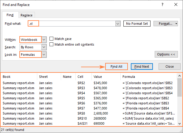
And these useful tips will help you manage the results:
- To select acell that contains an external link, click the cell address in the Cell
- To group the found links the way you want, click the corresponding column header, for example, Sheet or Formula.
- To select all cells with external references, place the cursor anywhere within the results and press Ctrl + A . This will select both the results in the Find and Replace dialog box and the cells in the workbook.
Note. With Find and Replace you can only identify external links in cells. If you’ve removed all external references from formulas but Excel still says there are links to external workbooks, then check other possible locations discussed below.
How to find links in Excel named ranges (defined names)
Excel pros often name ranges and individual cells to make their formulas easier to write, read, and understand. Data validation drop-down lists are also easier to create with named ranges, which in turn may refer to outside data. To take care of such cases, check for external links in Excel names:
- On the Formulas tab, in the Defined Names group, click Name Manager or press the Ctrl + F3 key combination.
- In the list of names, check the Refers Tocolumn for external links. References to other workbooks are enclosed in square brackets like [Source_data.xlsx].

How to identify external links in Excel objects
If you’ve linked objects such as shapes, text boxes, WordArt and the like to other Excel files, then you can use the Go To Special feature to locate such links:
- On the Hometab, in the Formats group, click Find & Select >Go to Special. Or press F5 to open for the Go To dialog, and then click Special… .
- In the Go To Special dialog box, select Objects and click OK. This will select all objects on the active sheet.
- Press the Tab key to cycle through the selected objects and check each individual object for references to other workbooks.

If an object is linked to a specific cell, you can see an external reference in the formula bar: 
If an object is linked to a file, then hover over the object with your mouse to see where it points to: 
Note. If an object is linked to a whole file rather than an individual cell, such link cannot be broken by using the Edit Links feature. To remove the link, right-click the object and select Remove link from the context menu.
How to find links to other files in Excel charts
In case external links are used in a chart title or data series, you can locate them in this way:
- On the graph, click the chart title or data series you wish to check.
- In the formula bar, look for a reference to another Excel file.
External reference in chart title: 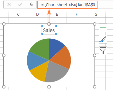
External link in chart data series: 
If your chart contains several data series, you can quickly move between them in this way:
- Select the target chart.
- Go to the Format tab >Current Selection group, click the arrow next to the Chart Elements box, and select the data series of interest.

How to find external links in Pivot Tables
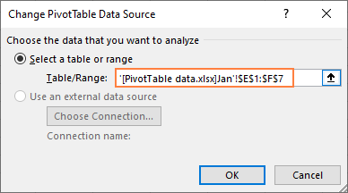
Most often a PivotTable is created using the data in the same workbook. But sometimes, the source data resides in an outside file. To find the exact location of your PivotTable’s source data, perform these steps:
- Click any cell within the Pivot Table.
- On the PivotTable Analyze tab, in the Data group, click the Change Data Source button.
- In the dialog box that appears, check the data source in the Table/Range box to see whether it is linked externally.

How to enable links to external workbooks in Excel
When you open a workbook with links to other files for the first time, Excel shows a security warning informing you that the file contains links to external data. To allow the links to update, simply click the Enable Content button. 
On subsequent openings of the same file, you will be presented with the following prompt asking if you want to update the links. If you trust the linked documents and want to pull the latest data, click Update. 
Control the security prompt about updating links
By default, Excel asks whether or not to update external references every time you open a workbook. However, you can control whether the message appears and whether the links are updated or not.
- On the Datatab, in the Queries & Connections group, click Edit Links.
- In the lower-left corner of the Edit Links dialog box, click Startup Prompt….
- In the Startup Prompt dialog box, choose the option that works best for you:
- Let users choose to display the alert or not (default).
- Don’t display the alert and don’t update automatic links — it makes sense to choose this option when you are sharing a workbook with other people who do not have access to the source files.
- Don’t display the alert and update links — you can choose this setting when you completely trust the sources.


Change security setting for external links
You can also set links to other files to be updated automatically in a particular workbook without getting a security warning by changing the Trust Center security settings:
- In the target workbook, click the File tab >Options.
- In the Excel Options dialog box, click Trust Center >Trust Center Settings.
- In the Trust Center dialog box, click External Content, and then select Enable automatic update for all Workbook Links under Security settings for Workbook Links.

With this option turned on, Excel will update all links to external sources in the current workbook automatically without showing you any warnings or prompts.

Please note that automatic updating of links to unknown files can be harmful and therefore is not recommended. Enable it only when you are 100% confident in the security of the outside data. Or, turn on this option temporarily, and then return to the default Prompt user on automatic update for Workbook Links setting.
Note. Regardless which option you choose, Excel will still display the below prompt if the workbook contains invalid or broken links.

How to break external links in Excel
In Excel, breaking a link to another workbook means replacing an external reference with its current value.
For example, if you break the following external reference, it will be replaced with the value that is currently in cell A1 on the Jan sheet in the Source data workbook:
If you break an external link in the below formula, the formula will be changed to its calculated value, whatever it is:
Note. Because breaking links is the action that cannot be undone, it may be wise to save a backup copy of your workbook first.
To break external links in Excel, this is what you need to do:
- On the Data tab, in the Queries &Connections group, click the Edit Links button.
If this button is greyed out, that means there is no linked data in your workbook.

- To select multiple links, click on each one individually while holding down the Ctrl key.
- To select all links, press the Ctrl + A shortcut .

Note. Under ideal circumstances, this feature should remove all external links in a workbook. Unfortunately, we do not live in a perfect world 🙁 Some links to outside data, e.g. external source data in Pivot Tables, are not shown in the Edit Links dialog while others cannot be broken. If the Edit Links button is grayed out in your workbook but you are still getting a prompt about external data, then you will have to check each possible place where external references may be lurking (such as objects, charts, etc.) and change or remove the links manually.
Get a list of all external links in a workbook
To get a list of all external sources that your workbook refers to, you can use one of the following methods.
Traditional approach
The conventional way to check links in Excel is by using the Edit Links feature: Data tab > Queries & Connections group > Edit Links.
This will display the following information:
- Source — the name of the linked file
- Type — the link type: a workbook or worksheet
- Update — whether the link updates automatically or manually
- Status — the status of the link such as OK, Source is Open, Warning, Unknown, etc. To get the most recent info, click the Check Status button on the right.

Very quick and straightforward, this method is not very convenient though. To see the location of the source file, you need to click each link, one at a time.
Dynamic arrays and Excel 4.0 macros.
A very cute trick suggested by Bob Ulmas in his book «This isn’t Excel, it’s Magic!» can help you retrieve the locations of all source files in one go. The solution combines the recently introduced dynamic arrays with the good old Excel 4.0 macros.
To generate a list of all external references in a given workbook, this is what you need to do:
Step 1. Create a new name that references the macro
To be able to use a built-in Excel 4.0 macro in a formula, you need to create a name referencing the macro. Here’s how:
- On the Formulas tab, in the Defined Names group, click Name Manager. Or simply press the Ctrl + F3 shortcut.
- In the Name Manager dialog window, click the New…
- In the New Name dialog window, type some meaningful name, say GetLinks, in the Name box and the following formula in the Refers to box: =LINKS()
- Click OK.

For more detailed instructions, please see How to create a name in Excel.
Step 2. Use the newly create name in a formula
Now that you have a name that references the macro, you just need to put the name in a formula. Depending on your Excel version, the formula will take a different form.
In the topmost cell of the destination range, enter this formula:
GetLinks (or any other name that you utilized for referencing the macro) returns a horizontal spill range of all the external links in the workbook. The TRANSPOSE function rotates rows to columns and outputs a vertical list that is easier to read. 
To arrange the list in alphabetical order, put the above formula inside the SORT function:
Please remember that this solution only works in Excel 365 that has a new calculation engine supporting dynamic arrays.
In Excel 2019 — 2007:
In pre-dynamic versions of Excel, use the GetLinks name for the array argument of the classic INDEX function. To make the solution more user-friendly, you can wrap the construction in IFERROR to take care of situations when the formula is copied to more cells than there are external references in your workbook:
The formula goes to the first cell (A2), and then you drag it down to the below cells: 
- Because this solution uses macros, the file must be saved as a Macro-Enabled Workbook (.xlsm).
- Excel macros do not execute nor update automatically. To refresh a list of links, press the Ctrl + Alt + F9 keys shortcut, which recalculates all formulas in all open workbooks.
VBA macro to get a list of external links
If you have nothing against using macros in your worksheets, the following VBA code can find and list down all links to external sources in a workbook automatically:
To add the code to your workbook, do the following:
- Press Alt + F11 to open the Visual Basic Editor.
- On the left pane, right-click ThisWorkbook, and then click Insert >Module.
- Paste the above code in the Code window.
For the detailed steps, please see How to insert VBA code in Excel.
To run the macro, press either Alt + F8 in a workbook or F5 in the VBA Editor.
For more information, please see How to run macro in Excel.
As the result, you will get a list of external sources in a new sheet: 
Find cells with external links using VBA
If your goal is to get a complete list of all external references in a workbook including the addresses of the cells containing the links, the following code can be helpful. Here, we utilize the LinkSources method to get all source workbooks and the LinkInfo method to identify their status. The status of a link is determined as described on this page:
https://docs.microsoft.com/en-us/office/vba/api/excel.xllinkstatus
The results are output in a new worksheet named All Links report. Column B contains hyperlinks to the cells with outside links. 
To make use of the code straight away, you can download our sample workbook at the end of the post. The workbook contains the above code as well as the detailed step-by-step instructions on how to run it.
Find all external links in a workbook in a click
Reading the previous examples, perhaps you were wondering why simple things need to be made so complicated. We also asked that question to ourselves… and implemented a one-click solution for this task.
With Ultimate Suite installed in your Excel, finding all links in a workbook takes a single click on the Find Links button: 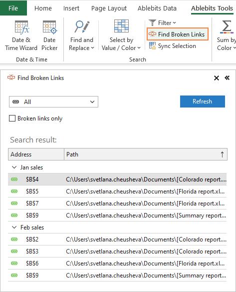
By default, the tool looks for all links: internal, external and web pages. To display only external references, select this option in the drop-down list and click the Refresh button. 
To show only broken links, just put a tick in the corresponding check box.
To get to a cell that references external data, click the cell address on the pane.
Simple things should be kept simple! 🙂
That’s how to find links to external sources in Excel. I thank you for reading and hope to see you on our blog next week!
Источник
Insert a link to a file
- Click inside the cell of the spreadsheet where you want to insert the object.
- On the Insert tab, in the Text group, click Object.
- Click the Create from File tab.
- Click Browse, and then select the file you want to link.
- Select the Link to file check box, and click OK.
Contents
- 1 How do I Link a file path in Excel?
- 2 What is an Xlookup in Excel?
- 3 How do I create a link to a file?
- 4 How do I turn a file into a hyperlink?
- 5 How do I enable Xlookup?
- 6 Is Xlookup better than VLOOKUP?
- 7 How do I share files?
- 8 How do I create a Link to a folder?
- 9 Is Xlookup available in Excel 2021?
- 10 Why does my excel not have Xlookup?
- 11 What version of Excel is Xlookup available?
- 12 Is Xlookup new?
- 13 Why would you use VLOOKUP over Xlookup?
- 14 Does Google sheets have Xlookup?
- 15 How do I share a link?
- 16 How do I share files between computers?
- 17 How do I share files on one drive?
How do I Link a file path in Excel?
In the Insert Hyperlink dialog box, click Existing File or Web Page in the Link to section, then paste the folder path you have copied into the Address box, and finally click the OK button.
What is an Xlookup in Excel?
Use the XLOOKUP function to find things in a table or range by row.With XLOOKUP, you can look in one column for a search term, and return a result from the same row in another column, regardless of which side the return column is on.
How do I create a link to a file?
Hold down Shift on your keyboard and right-click on the file, folder, or library for which you want a link. Then, select “Copy as path” in the contextual menu. If you’re using Windows 10, you can also select the item (file, folder, library) and click or tap on the “Copy as path” button from File Explorer’s Home tab.
How do I turn a file into a hyperlink?
Try it!
- Select what you’d like to turn into a link and then select Insert > Hyperlink or press Ctrl + K.
- Select Place in This Document.
- Choose where you’d like the link to connect to and select OK.
How do I enable Xlookup?
- Position the cell cursor in cell E4 of the worksheet.
- Click the Lookup & Reference option on the Formulas tab followed by XLOOKUP near the bottom of the drop-down menu to open its Function Arguments dialog box.
- Click cell D4 in the worksheet to enter its cell reference into the Lookup_value argument text box.
Is Xlookup better than VLOOKUP?
The XLOOKUP defaults to an exact match where the VLOOKUP defaults to an approximate match. As the exact match is used most often, this setting would make the XLOOKUP more effective. On top of this, the XLOOKUP offers an additional option of an approximate match returning the next larger value.
Share with specific people
- Select the file you want to share.
- Click Share or Share .
- Under “Share with people and groups,” enter the email address you want to share with.
- To change what people can do to your doc, on the right, click the Down arrow.
- Choose to notify people.
- Click Share or Send.
How do I create a Link to a folder?
Right click on any file or folder in your Sync folder. Select Create a Link from the file menu. The link will be copied your clipboard. You can then paste it into an email (Gmail, Outlook, Office 365, Apple Mail etc.), into a message, onto a website, or wherever you want people to access it.
Is Xlookup available in Excel 2021?
Excel 2021 for Windows allows you to collaboratively work with others and analyze data easily with new Excel capabilities including co-authoring, Dynamic Arrays, XLOOKUP, and LET functions.
Why does my excel not have Xlookup?
XLOOKUP was introduced after Excel 2019 was launched. All new functions come only in Office 365. Hence, you won’t have XLOOKUP in Excel 2019. When new version of Excel is launched say Excel 2022, then all new functions rolled between Excel 2019 and launch of Excel 2022 will become part of Excel 2022.
What version of Excel is Xlookup available?
Office 365
What Versions of Excel Will Have XLOOKUP? Only Excel for Office 365 will get the new XLOOKUP function. Excel 2019 and all previous versions won’t ever get this new function.
Is Xlookup new?
Fortunately, the geniuses on the Microsoft Excel team have just released XLOOKUP, a brand-new function available in Office 365* that replaces VLOOKUP. (It also replaces HLOOKUP, the lesser-used function for searching horizontally, in spreadsheet rows.)
Why would you use VLOOKUP over Xlookup?
XLOOKUP requires referencing fewer cells. VLOOKUP required you to input an entire data set, but XLOOKUP only requires you to reference the relevant columns or rows. By referencing fewer cells, the XLOOKUP will increase your spreadsheet calculation speed and potentially result in fewer circular reference errors.
Does Google sheets have Xlookup?
XLOOKUP for google sheets is a custom function that comes handy when you want to search for things from a table or range using another row.
Done.
- Select the file you want to share.
- Tap Share or Share .
- Under “Get Link,” tap Link settings .
- Select Public link. Save.
- Tap Done.
- Copy and paste the link in an email or any place you want to share it.
To do this, open File Explorer, right-click the file you want to share, and select Sharing. Now you’ll see all computers with Nearby Sharing enabled under the Find more people section. When you select that remote computer system, a notification will appear on the other computer that there’s an incoming file.
Share files or photos in email
- Select the files or photos you want to share, and then select Share .
- Choose if you want to allow Allow editing.
- Select Email.
- Enter the email addresses of the people you’d like to share with and add an optional message.
- Select Share. Everyone you share with will receive an email.
See all How-To Articles
This tutorial demonstrates how to link Excel files or Google Sheets.
Link Files in Excel
In your Excel file, you can easily link a cell to another workbook using links. This works the same as inserting hyperlinks in your document.
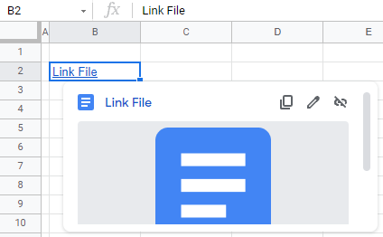
- Select the cell where you want to insert a link (here, B2), and in the Ribbon, go to Insert > Link. You can also right-click the cell and choose Link (or use the keyboard shortcut CTRL + K).
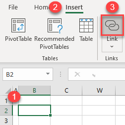
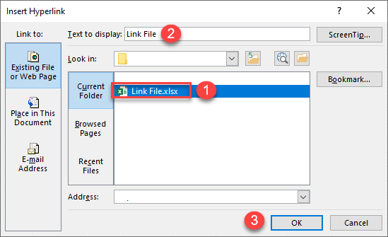
- The Insert Hyperlink window opens to the Existing File or Web Page tab. Choose the file to link to (here, Link File.xlsx).Then enter the Text to display– the text that appears on the link (here, Link File). Click OK.
By default, you’re taken to the same folder as the open workbook. To choose a file from a different folder, click the Browse icon. Similarly, you can link any other type of document (Word, PowerPoint, pictures, etc.).
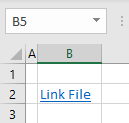
As a result, a link to the Link File.xlsx file is inserted in cell B2. If you click on it, the file is opened in a new Excel window.
If you delete the linked file, you’ll get an error message when you click on the link. You can also use VBA to insert hyperlinks and link to another file in Excel.
Link Files in Google Sheets
Since all Google Docs and Google Sheets files are stored in Google Drive, you can’t browse for them in folders, so you need to use a hyperlink to another file’s URL. To link a Google doc from a Google sheet, follow these steps:
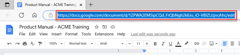
- Copy the URL of your Google doc.
You can find it in the address bar on your browser.
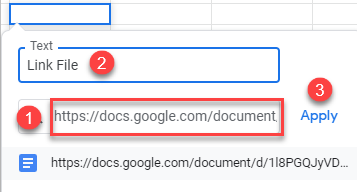
- In your spreadsheet, select the cell where you want to insert a link to a file and in the Menu, go to Insert > Insert link. You can also right-click the cell and choose Link (or use the keyboard shortcut CTRL + K).
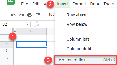
- In the pop-up window, paste the link you copied, enter the text to display in the cell, and click Apply.
If you don’t put anything in the Text field (labeled 2 below), the full link to the file in Google Drive is displayed.
As a result, the link to the file is inserted in cell B2. When you position your cursor over the cell, you can see the link and a preview of the document.