Links in excel sheet - Word и Excel - помощь в работе с программами

For quick access to related information in another file or on a web page, you can insert a hyperlink in a worksheet cell. You can also insert links in specific chart elements.

Note: Most of the screen shots in this article were taken in Excel 2016. If you have a different version your view might be slightly different, but unless otherwise noted, the functionality is the same.

On a worksheet, click the cell where you want to create a link.

You can also select an object, such as a picture or an element in a chart, that you want to use to represent the link.
- On the Insert tab, in the Links group, click Link .
You can also right-click the cell or graphic and then click Link on the shortcut menu, or you can press Ctrl+K.
Under Link to, click Create New Document.
In the Name of new document box, type a name for the new file.

Tip: To specify a location other than the one shown under Full path, you can type the new location preceding the name in the Name of new document box, or you can click Change to select the location that you want and then click OK.
Under When to edit, click Edit the new document later or Edit the new document now to specify when you want to open the new file for editing.
In the Text to display box, type the text that you want to use to represent the link.
To display helpful information when you rest the pointer on the link, click ScreenTip, type the text that you want in the ScreenTip text box, and then click OK.

On a worksheet, click the cell where you want to create a link.

You can also select an object, such as a picture or an element in a chart, that you want to use to represent the link.
- On the Insert tab, in the Links group, click Link .
You can also right-click the cell or object and then click Link on the shortcut menu, or you can press Ctrl+K.
Under Link to, click Existing File or Web Page.
Do one of the following:
- To select a file, click Current Folder, and then click the file that you want to link to.
  
  You can change the current folder by selecting a different folder in the Look in list.
- To select a web page, click Browsed Pages and then click the web page that you want to link to.
- To select a file that you recently used, click Recent Files, and then click the file that you want to link to.
- To enter the name and location of a known file or web page that you want to link to, type that information in the Address box.
- To locate a web page, click Browse the Web , open the web page that you want to link to, and then switch back to Excel without closing your browser.
If you want to create a link to a specific location in the file or on the web page, click Bookmark, and then double-click the bookmark that you want.

Note: The file or web page that you are linking to must have a bookmark.
In the Text to display box, type the text that you want to use to represent the link.
To display helpful information when you rest the pointer on the link, click ScreenTip, type the text that you want in the ScreenTip text box, and then click OK.

To link to a location in the current workbook or another workbook, you can either define a name for the destination cells or use a cell reference.

To use a name, you must name the destination cells in the destination workbook.

How to name a cell or a range of cells
1. Select the cell, range of cells, or nonadjacent selections that you want to name.
2. Click the Name box at the left end of the formula bar .
  
  Name box
3. In the Name box, type the name for the cells, and then press Enter.
  
  Note: Names can’t contain spaces and must begin with a letter.
On a worksheet of the source workbook, click the cell where you want to create a link.

You can also select an object, such as a picture or an element in a chart, that you want to use to represent the link.
- On the Insert tab, in the Links group, click Link .
You can also right-click the cell or object and then click Link on the shortcut menu, or you can press Ctrl+K.
Under Link to, do one of the following:
- To link to a location in your current workbook, click Place in This Document.
- To link to a location in another workbook, click Existing File or Web Page, locate and select the workbook that you want to link to, and then click Bookmark.
Do one of the following:
- In the Or select a place in this document box, under Cell Reference, click the worksheet that you want to link to, type the cell reference in the Type in the cell reference box, and then click OK.
- In the list under Defined Names, click the name that represents the cells that you want to link to, and then click OK.
In the Text to display box, type the text that you want to use to represent the link.
To display helpful information when you rest the pointer on the link, click ScreenTip, type the text that you want in the ScreenTip text box, and then click OK.

You can use the HYPERLINK function to create a link that opens a document that is stored on a network server, an intranet, or the Internet. When you click the cell that contains the HYPERLINK function, Excel opens the file that is stored at the location of the link.

Syntax

HYPERLINK(link_location,friendly_name)

Link_location is the path and file name to the document to be opened as text. Link_location can refer to a place in a document — such as a specific cell or named range in an Excel worksheet or workbook, or to a bookmark in a Microsoft Word document. The path can be to a file stored on a hard disk drive, or the path can be a universal naming convention (UNC) path on a server (in Microsoft Excel for Windows) or a Uniform Resource Locator (URL) path on the Internet or an intranet.

Link_location can be a text string enclosed in quotation marks or a cell that contains the link as a text string.
If the jump specified in link_location does not exist or can’t be navigated, an error appears when you click the cell.

Friendly_name is the jump text or numeric value that is displayed in the cell. Friendly_name is displayed in blue and is underlined. If friendly_name is omitted, the cell displays the link_location as the jump text.

Friendly_name can be a value, a text string, a name, or a cell that contains the jump text or value.
If friendly_name returns an error value (for example, #VALUE!), the cell displays the error instead of the jump text.

Examples

The following example opens a worksheet named Budget Report.xls that is stored on the Internet at the location named example.microsoft.com/report and displays the text «Click for report»:

=HYPERLINK(«http://example.microsoft.com/report/budget report.xls», «Click for report»)

The following example creates a link to cell F10 on the worksheet named Annual in the workbook Budget Report.xls, which is stored on the Internet at the location named example.microsoft.com/report. The cell on the worksheet that contains the link displays the contents of cell D1 as the jump text:

=HYPERLINK(«[http://example.microsoft.com/report/budget report.xls]Annual!F10», D1)

The following example creates a link to the range named DeptTotal on the worksheet named First Quarter in the workbook Budget Report.xls, which is stored on the Internet at the location named example.microsoft.com/report. The cell on the worksheet that contains the link displays the text «Click to see First Quarter Department Total»:

=HYPERLINK(«[http://example.microsoft.com/report/budget report.xls]First Quarter!DeptTotal», «Click to see First Quarter Department Total»)

To create a link to a specific location in a Microsoft Word document, you must use a bookmark to define the location you want to jump to in the document. The following example creates a link to the bookmark named QrtlyProfits in the document named Annual Report.doc located at example.microsoft.com:

=HYPERLINK(«[http://example.microsoft.com/Annual Report.doc]QrtlyProfits», «Quarterly Profit Report»)

In Excel for Windows, the following example displays the contents of cell D5 as the jump text in the cell and opens the file named 1stqtr.xls, which is stored on the server named FINANCE in the Statements share. This example uses a UNC path:

=HYPERLINK(«\FINANCEStatements1stqtr.xls», D5)

The following example opens the file 1stqtr.xls in Excel for Windows that is stored in a directory named Finance on drive D, and displays the numeric value stored in cell H10:

=HYPERLINK(«D:FINANCE1stqtr.xls», H10)

In Excel for Windows, the following example creates a link to the area named Totals in another (external) workbook, Mybook.xls:

=HYPERLINK(«[C:My DocumentsMybook.xls]Totals»)

In Microsoft Excel for the Macintosh, the following example displays «Click here» in the cell and opens the file named First Quarter that is stored in a folder named Budget Reports on the hard drive named Macintosh HD:

=HYPERLINK(«Macintosh HD:Budget Reports:First Quarter», «Click here»)

You can create links within a worksheet to jump from one cell to another cell. For example, if the active worksheet is the sheet named June in the workbook named Budget, the following formula creates a link to cell E56. The link text itself is the value in cell E56.

=HYPERLINK(«[Budget]June!E56», E56)

To jump to a different sheet in the same workbook, change the name of the sheet in the link. In the previous example, to create a link to cell E56 on the September sheet, change the word «June» to «September.»

When you click a link to an email address, your email program automatically starts and creates an email message with the correct address in the To box, provided that you have an email program installed.

On a worksheet, click the cell where you want to create a link.

You can also select an object, such as a picture or an element in a chart, that you want to use to represent the link.
- On the Insert tab, in the Links group, click Link .
You can also right-click the cell or object and then click Link on the shortcut menu, or you can press Ctrl+K.
Under Link to, click E-mail Address.
In the E-mail address box, type the email address that you want.
In the Subject box, type the subject of the email message.

Note: Some web browsers and email programs may not recognize the subject line.
In the Text to display box, type the text that you want to use to represent the link.
To display helpful information when you rest the pointer on the link, click ScreenTip, type the text that you want in the ScreenTip text box, and then click OK.

You can also create a link to an email address in a cell by typing the address directly in the cell. For example, a link is created automatically when you type an email address, such as someone@example.com.

You can insert one or more external reference (also called links) from a workbook to another workbook that is located on your intranet or on the Internet. The workbook must not be saved as an HTML file.

Open the source workbook and select the cell or cell range that you want to copy.
On the Home tab, in the Clipboard group, click Copy.
Switch to the worksheet that you want to place the information in, and then click the cell where you want the information to appear.
On the Home tab, in the Clipboard group, click Paste Special.
Click Paste Link.

Excel creates an external reference link for the cell or each cell in the cell range.

Note: You may find it more convenient to create an external reference link without opening the workbook on the web. For each cell in the destination workbook where you want the external reference link, click the cell, and then type an equal sign (=), the URL address, and the location in the workbook. For example:

=’http://www.someones.homepage/[file.xls]Sheet1′!A1

=’ftp.server.somewhere/file.xls’!MyNamedCell

To select a hyperlink without activating the link to its destination, do one of the following:

Click the cell that contains the link, hold the mouse button until the pointer becomes a cross , and then release the mouse button.
Use the arrow keys to select the cell that contains the link.
If the link is represented by a graphic, hold down Ctrl, and then click the graphic.

You can change an existing link in your workbook by changing its destination, its appearance, or the text or graphic that is used to represent it.

Change the destination of a link

Select the cell or graphic that contains the link that you want to change.

Tip: To select a cell that contains a link without going to the link destination, click the cell and hold the mouse button until the pointer becomes a cross , and then release the mouse button. You can also use the arrow keys to select the cell. To select a graphic, hold down Ctrl and click the graphic.
- On the Insert tab, in the Links group, click Link.
You can also right-click the cell or graphic and then click Edit Link on the shortcut menu, or you can press Ctrl+K.
In the Edit Hyperlink dialog box, make the changes that you want.

Note: If the link was created by using the HYPERLINK worksheet function, you must edit the formula to change the destination. Select the cell that contains the link, and then click the formula bar to edit the formula.

You can change the appearance of all link text in the current workbook by changing the cell style for links.

On the Home tab, in the Styles group, click Cell Styles.
Under Data and Model, do the following:
- To change the appearance of links that have not been clicked to go to their destinations, right-click Link, and then click Modify.
- To change the appearance of links that have been clicked to go to their destinations, right-click Followed Link, and then click Modify.
  
  Note: The Link cell style is available only when the workbook contains a link. The Followed Link cell style is available only when the workbook contains a link that has been clicked.
In the Style dialog box, click Format.
On the Font tab and Fill tab, select the formatting options that you want, and then click OK.
Notes:
- The options that you select in the Format Cells dialog box appear as selected under Style includes in the Style dialog box. You can clear the check boxes for any options that you don’t want to apply.
- Changes that you make to the Link and Followed Link cell styles apply to all links in the current workbook. You can’t change the appearance of individual links.

Select the cell or graphic that contains the link that you want to change.

Tip: To select a cell that contains a link without going to the link destination, click the cell and hold the mouse button until the pointer becomes a cross , and then release the mouse button. You can also use the arrow keys to select the cell. To select a graphic, hold down Ctrl and click the graphic.
Do one or more of the following:
- To change the link text, click in the formula bar, and then edit the text.
- To change the format of a graphic, right-click it, and then click the option that you need to change its format.
- To change text in a graphic, double-click the selected graphic, and then make the changes that you want.
- To change the graphic that represents the link, insert a new graphic, make it a link with the same destination, and then delete the old graphic and link.

Right-click the hyperlink that you want to copy or move, and then click Copy or Cut on the shortcut menu.
Right-click the cell that you want to copy or move the link to, and then click Paste on the shortcut menu.

By default, unspecified paths to hyperlink destination files are relative to the location of the active workbook. Use this procedure when you want to set a different default path. Each time that you create a link to a file in that location, you only have to specify the file name, not the path, in the Insert Hyperlink dialog box.

Follow one of the steps depending on the Excel version you are using:

In Excel 2016, Excel 2013, and Excel 2010:
1. Click the File tab.
2. Click Info.
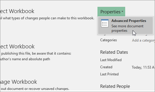
3. Click Properties, and then select Advanced Properties.
4. In the Summary tab, in the Hyperlink base text box, type the path that you want to use.
  
  Note: You can override the link base address by using the full, or absolute, address for the link in the Insert Hyperlink dialog box.
In Excel 2007:
1. Click the Microsoft Office Button , click Prepare, and then click Properties.
2. In the Document Information Panel, click Properties, and then click Advanced Properties.
3. Click the Summary tab.
4. In the Hyperlink base box, type the path that you want to use.
Note: You can override the link base address by using the full, or absolute, address for the link in the Insert Hyperlink dialog box.

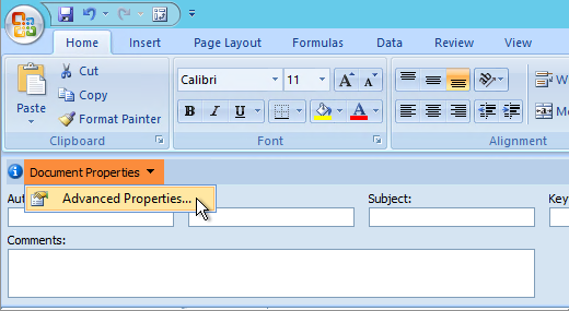
To delete a link, do one of the following:

To delete a link and the text that represents it, right-click the cell that contains the link, and then click Clear Contents on the shortcut menu.
To delete a link and the graphic that represents it, hold down Ctrl and click the graphic, and then press Delete.
To turn off a single link, right-click the link, and then click Remove Link on the shortcut menu.
To turn off several links at once, do the following:
1. In a blank cell, type the number 1.
2. Right-click the cell, and then click Copy on the shortcut menu.
3. Hold down Ctrl and select each link that you want to turn off.
  
  Tip: To select a cell that has a link in it without going to the link destination, click the cell and hold the mouse button until the pointer becomes a cross , and then release the mouse button.
4. On the Home tab, in the Clipboard group, click the arrow below Paste, and then click Paste Special.
5. Under Operation, click Multiply, and then click OK.
6. On the Home tab, in the Styles group, click Cell Styles.
7. Under Good, Bad, and Neutral, select Normal.

A link opens another page or file when you click it. The destination is frequently another web page, but it can also be a picture, or an email address, or a program. The link itself can be text or a picture.

When a site user clicks the link, the destination is shown in a Web browser, opened, or run, depending on the type of destination. For example, a link to a page shows the page in the web browser, and a link to an AVI file opens the file in a media player.

How links are used

You can use links to do the following:

Navigate to a file or web page on a network, intranet, or Internet
Navigate to a file or web page that you plan to create in the future
Send an email message
Start a file transfer, such as downloading or an FTP process

When you point to text or a picture that contains a link, the pointer becomes a hand , indicating that the text or picture is something that you can click.

What a URL is and how it works

When you create a link, its destination is encoded as a Uniform Resource Locator (URL), such as:

http://example.microsoft.com/news.htm

file://ComputerName/SharedFolder/FileName.htm

A URL contains a protocol, such as HTTP, FTP, or FILE, a Web server or network location, and a path and file name. The following illustration defines the parts of the URL:

1. Protocol used (http, ftp, file)

2. Web server or network location

3. Path

4. File name

Absolute and relative links

An absolute URL contains a full address, including the protocol, the Web server, and the path and file name.

A relative URL has one or more missing parts. The missing information is taken from the page that contains the URL. For example, if the protocol and web server are missing, the web browser uses the protocol and domain, such as .com, .org, or .edu, of the current page.

It is common for pages on the web to use relative URLs that contain only a partial path and file name. If the files are moved to another server, any links will continue to work as long as the relative positions of the pages remain unchanged. For example, a link on Products.htm points to a page named apple.htm in a folder named Food; if both pages are moved to a folder named Food on a different server, the URL in the link will still be correct.

In an Excel workbook, unspecified paths to link destination files are by default relative to the location of the active workbook. You can set a different base address to use by default so that each time that you create a link to a file in that location, you only have to specify the file name, not the path, in the Insert Hyperlink dialog box.

On a worksheet, select the cell where you want to create a link.
On the Insert tab, select Hyperlink.

You can also right-click the cell and then select Hyperlink… on the shortcut menu, or you can press Ctrl+K.
Under Display Text:, type the text that you want to use to represent the link.
Under URL:, type the complete Uniform Resource Locator (URL) of the webpage you want to link to.
Select OK.

To link to a location in the current workbook, you can either define a name for the destination cells or use a cell reference.

To use a name, you must name the destination cells in the workbook.

How to define a name for a cell or a range of cells

Note: In Excel for the Web, you can’t create named ranges. You can only select an existing named range from the Named Ranges control. Alternately, you can open the file in the Excel desktop app, create a named range there, and then access this option from Excel for the web.
1. Select the cell or range of cells that you want to name.
2. On the Name Box box at the left end of the formula bar , type the name for the cells, and then press Enter.
  
  Note: Names can’t contain spaces and must begin with a letter.
On the worksheet, select the cell where you want to create a link.
On the Insert tab, select Hyperlink.

You can also right-click the cell and then select Hyperlink… on the shortcut menu, or you can press Ctrl+K.
Under Display Text:, type the text that you want to use to represent the link.
Under Place in this document:, enter the defined name or cell reference.
Select OK.

On a worksheet, select the cell where you want to create a link.
On the Insert tab, select Hyperlink.

You can also right-click the cell and then select Hyperlink… on the shortcut menu, or you can press Ctrl+K.
Under Display Text:, type the text that you want to use to represent the link.
Under E-mail address:, type the email address that you want.
Select OK.

You can also create a link to an email address in a cell by typing the address directly in the cell. For example, a link is created automatically when you type an email address, such as someone@example.com.

You can use the HYPERLINK function to create a link to a URL.

Note: The Link_location can be a text string enclosed in quotation marks or a reference to a cell that contains the link as a text string.

To select a hyperlink without activating the link to its destination, do any of the following:

Select a cell by clicking it when the pointer is an arrow.
Use the arrow keys to select the cell that contains the link.

You can change an existing link in your workbook by changing its destination, its appearance, or the text that is used to represent it.

Select the cell that contains the link that you want to change.

Tip: To select a hyperlink without activating the link to its destination, use the arrow keys to select the cell that contains the link.
On the Insert tab, select Hyperlink.

You can also right-click the cell or graphic and then select Edit Hyperlink… on the shortcut menu, or you can press Ctrl+K.
In the Edit Hyperlink dialog box, make the changes that you want.

Note: If the link was created by using the HYPERLINK worksheet function, you must edit the formula to change the destination. Select the cell that contains the link, and then select the formula bar to edit the formula.

Right-click the hyperlink that you want to copy or move, and then select Copy or Cut on the shortcut menu.
Right-click the cell that you want to copy or move the link to, and then select Paste on the shortcut menu.

To delete a link, do one of the following:

To delete a link, select the cell and press Delete.
To turn off a link (delete the link but keep the text that represents it), right-click the cell and then select Remove Hyperlink.

Need more help?

You can always ask an expert in the Excel Tech Community or get support in the Answers community.

Things You Should Know

You can link to a new file, existing file, webpage, email, or location in your document.
Use the HYPERLINK function if you already have the link location.
Create an external reference link to another workbook to insert a cell value into your workbook.

1
Open an Excel document. Double-click the Excel document in which you want to insert a hyperlink.
- You can also open a new document by double-clicking the Excel icon and clicking Blank Workbook.
2

Select a cell. This should be a cell into which you want to insert your hyperlink.

Advertisement
3
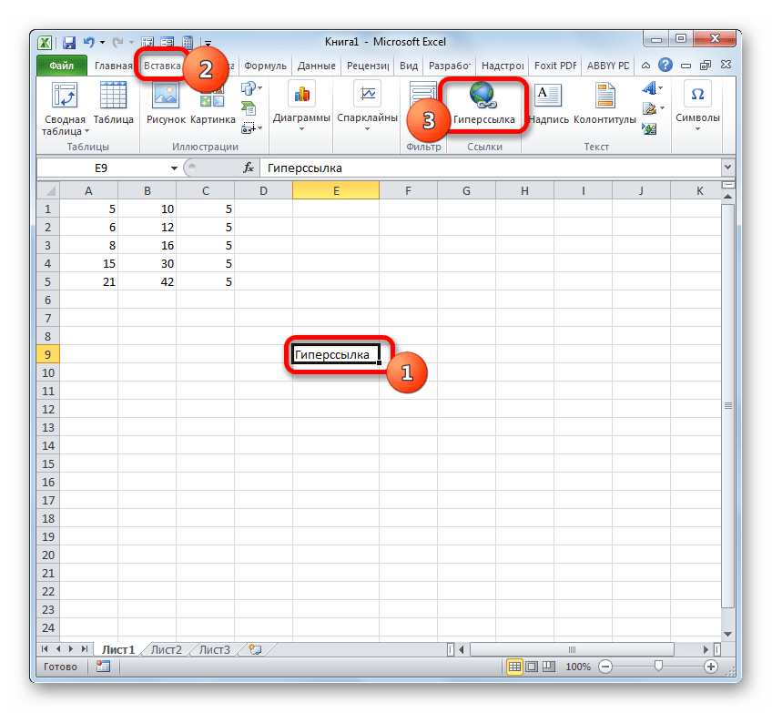
Click Insert. This tab is in the green ribbon at the top of the Excel window. Clicking Insert opens a toolbar directly below the green ribbon.^[1]
- If you’re on a Mac, note that there’s an Excel Insert tab and an Insert menu item in your Mac’s menu bar. Select the Excel Insert tab.
4

Click Link. It’s toward the right side of the Insert toolbar in the «Links» section. Doing so opens a pop up menu.
5

Click Insert Link. It’s at the bottom of the Link pop up menu. This opens the Insert Hyperlink window.
6
Click Create New Document. This tab is on the left side of the pop-up window, under “Link to:”.
- This option is not available on some versions of Excel. You’ll need to create the new document before making the hyperlink, then use the Existing File or Web Page option.
7

Enter the hyperlink’s text. Type the text that you want to see displayed into the «Text to display» field. This is the box above the “Name of new document” field.
8

Type in a name for the new document. Do so in the «Name of new document» field.
9
Click OK. It’s at the bottom of the window. By default, this will create and open a new spreadsheet document, then create a link to it in the cell that you selected in the other spreadsheet document.
- You can also select the «Edit the new document later» option before clicking OK to create the spreadsheet and the link without opening the spreadsheet.
- If something goes wrong with the hyperlink, see our guide for fixing a hyperlink in Excel.

1
Open an Excel document. Double-click the Excel document in which you want to insert a hyperlink.
- You can also open a new document by double-clicking the Excel icon and then clicking Blank Workbook.
- Hyperlinks are a great way to organize and connect information across multiple Excel documents. You can also easily create hyperlinks in PowerPoint if you have a presentation coming up.
2

Select a cell. This should be a cell into which you want to insert your hyperlink.
3
Click Insert. This tab is in the green ribbon at the top of the Excel window. Clicking Insert opens a toolbar directly below the green ribbon.
- If you’re on a Mac, note that there’s an Excel Insert tab and an Insert menu item in your Mac’s menu bar. Select the Excel Insert tab.
4

Click Link. It’s toward the right side of the Insert toolbar in the «Links» section. Doing so opens a pop up menu.
5

Click Insert Link. It’s at the bottom of the Link pop up menu. This opens the Insert Hyperlink window.
6

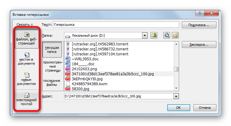
Click the Existing File or Web Page. It’s on the left side of the window.
7
Enter the hyperlink’s text. Type the text that you want to see displayed into the «Text to display» field.
- If you don’t do this, your hyperlink’s text will just be the folder path to the linked item.
8
Select a destination. You can choose a file location on your computer, enter an address of a file or web page, or browse the internet. Here are the destination options:
- Current Folder — Search for files in your Documents or Desktop folder.
- Browsed Pages — Search through recently viewed web pages.
- Recent Files — Search through recently opened Excel files.
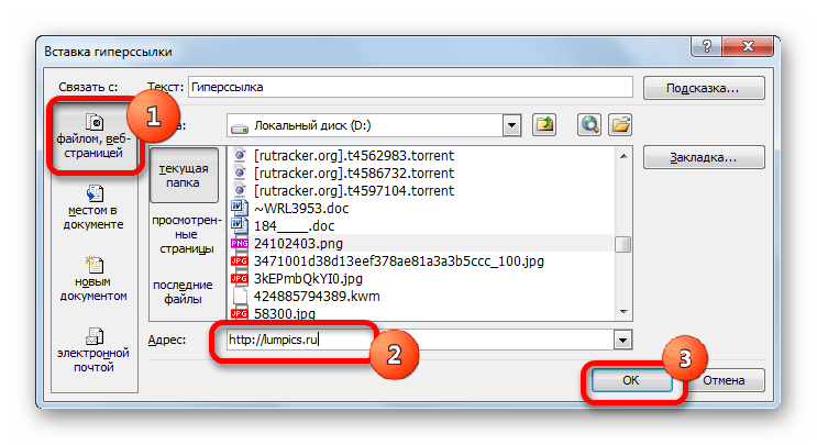
- Type in the location and name of a web page or file into the “Address” field. For example, this could be a URL to a website.
- Click the Browse the Web button (a globe behind a magnifying glass). Go to the web page you’re linking to, then go back to Excel. Don’t close your browser!
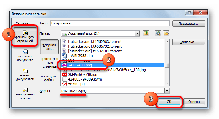
9

Select a file or webpage. Click the file, folder, or web address to which you want to link. A path to the folder will appear in the «Address» text box at the bottom of the window.
10
Click OK. It’s at the bottom of the page. Doing so creates your hyperlink in your specified cell.
- Note that if you move the item to which you linked, the hyperlink will no longer work.

1
Open an Excel document. Double-click the Excel document in which you want to insert a hyperlink. This method links to a cell or sheet in your workbook. For example, if you’re tracking your bills in Excel, you can link to a summary sheet from your data sheet.
- You can also open a new document by double-clicking the Excel icon and then clicking Blank Workbook.
2

Select a cell. This should be a cell into which you want to insert your hyperlink.
3
Click Insert. This tab is in the green ribbon at the top of the Excel window. Clicking Insert opens a toolbar directly below the green ribbon.
- If you’re on a Mac, note that there’s an Excel Insert tab and an Insert menu item in your Mac’s menu bar. Select the Excel Insert tab.
4

Click Link. It’s toward the right side of the Insert toolbar in the «Links» section. Doing so opens a pop up menu.
5

Click Insert Link. It’s at the bottom of the Link pop up menu. This opens the Insert Hyperlink window.
6

Click the Place in This Document. It’s on the left side of the window.
7
Select a location in the Excel document. You have two options for selecting a location:
- Under “Type the cell reference,” type in the cell you want to link to.
- Alternatively, under “Or select a place in this document,” click a sheet name or defined name.
8
Enter the hyperlink’s text. Type the text that you want to see displayed into the «Text to display» field.
- If you don’t do this, your hyperlink’s text will just be the linked cell’s name.
9
Click OK. This will create your link in the selected cell. If you click the hyperlink, Excel will automatically highlight the linked cell or take you to the sheet you selected.
- For general Excel tips, see our intro guide to Excel.

1
Open an Excel document. Double-click the Excel document in which you want to insert a hyperlink.
- You can also open a new document by double-clicking the Excel icon and then clicking Blank Workbook.
2

Select a cell. This should be a cell into which you want to insert your hyperlink.
3
Click Insert. This tab is in the green ribbon at the top of the Excel window. Clicking Insert opens a toolbar directly below the green ribbon.
- If you’re on a Mac, note that there’s an Excel Insert tab and an Insert menu item in your Mac’s menu bar. Select the Excel Insert tab.
4

Click Link. It’s toward the right side of the Insert toolbar in the «Links» section. Doing so opens a pop up menu.
5

Click Insert Link. It’s at the bottom of the Link pop up menu. This opens the Insert Hyperlink window.
6

Click E-mail Address. It’s on the left side of the window.
7
Enter the hyperlink’s text. Type the text that you want to see displayed into the «Text to display» field.
- If you don’t change the hyperlink’s text, the email address will display as itself.
8
Enter the email address. Type the email address that you want to hyperlink into the «E-mail address» field.
- You can also add a prewritten subject to the «Subject» field, which will cause the hyperlinked email to open a new email message with the subject already filled in.
9
Click OK. This button is at the bottom of the window.
- Clicking this email link will automatically open an installed email program with a new email to the specified address.

1
Open an Excel document. Double-click the Excel document in which you want to insert a hyperlink.
- You can also open a new document by double-clicking the Excel icon and then clicking Blank Workbook.
2

Select a cell. This should be a cell into which you want to insert your hyperlink.
3
Type =HYPERLINK(). This function creates a hyperlink to a document on the Internet, an intranet, or a server. This function has two parameters:^[2]
- HYPERLINK(link_location,friendly_name)
- link_location is where you type in the path to the file and the file name.
- friendly_name is the text shown for the hyperlink in your Excel spreadsheet. This parameter is optional.
4
Add the link location and friendly name. To do so:
- In the parenthesis of the HYPERLINK function, type the file path and file name for the document you want to link to.
- Add a comma (,).
- Type the name you want to appear for the hyperlink.
5

Press ↵ Enter. This will confirm the HYPERLINK formula and create the hyperlink in the selected cell. Clicking the link will open the specified file.

1
Open an Excel document. Double-click the Excel document in which you want to insert a hyperlink.
- You can also open a new document by double-clicking the Excel icon and then clicking Blank Workbook.
2

Open the workbook you want to link to. This can be referred to as the source workbook. This method creates an external reference link to a workbook on the Internet or your intranet.
3

Select the cell you want to link to in the source workbook. This will place a green box around the cell.
4
Copy the cell. You’ll need to copy the cell to reference it in your workbook. To copy it:
- Go to the Home tab.
- Click Copy in the “Clipboard” section. This button has an icon of two pieces of paper.
5

Go to your workbook. This is the workbook that you want to place the external reference link in.
6

Select the cell you want to place the link in. You can place the link in any sheet of your workbook.
7

Click the Home tab. This will open the Home toolbar.
8

Click the Paste drop down button. This is the button below the clipboard with a down arrow. This opens the Paste drop down menu.
9
Click the Paste Link button. This is two chains linked together in front of a clipboard in the Paste drop down menu. The value of the external reference will appear in the cell you selected.
- To see the external reference location, select the cell with the external reference. Then, check the Formula Bar for the location.

Add New Question

Question

How do I put a hyperlink in a text box?

Right-click on the cell into which you wish to insert the link. Choose ‘Link’ on the menu which pops up, then insert the URL at the bottom of the little Link Setup Window.
Question

My Excel chart hyperlinks work on my computer, but not on the computers of folks I send the chart to. Why?

MS Office applications routinely disable links and other potentially harmful content whenever you open a file created on another PC or downloaded from the Internet. A warning message is displayed at the top of the document. The user then has the choice to trust the source of the document, which enables all content, or to view it in «Compatibility Mode,» with potentially harmful content disabled.
Question

The hyperlink option in the drop down menu is shaded and I can’t click on it. What should I do?

Highlight the text you want to add a hyperlink to, then click hyperlink.

Ask a Question

200 characters left

Include your email address to get a message when this question is answered.

Submit

Video

Thanks for submitting a tip for review!

If you move a file connected to an Excel spreadsheet by hyperlink to a new location, you will have to edit the hyperlink to include the new file location.

About This Article

Thanks to all authors for creating a page that has been read 486,649 times.

Is this article up to date?

Источник

Содержание

Создание различных типов ссылок
- Способ 1: создание ссылок в составе формул в пределах одного листа
- Способ 2: создание ссылок в составе формул на другие листы и книги
- Способ 3: функция ДВССЫЛ
- Способ 4: создание гиперссылок
Вопросы и ответы

Ссылки — один из главных инструментов при работе в Microsoft Excel. Они являются неотъемлемой частью формул, которые применяются в программе. Иные из них служат для перехода на другие документы или даже ресурсы в интернете. Давайте выясним, как создать различные типы ссылающихся выражений в Экселе.

Создание различных типов ссылок

Сразу нужно заметить, что все ссылающиеся выражения можно разделить на две большие категории: предназначенные для вычислений в составе формул, функций, других инструментов и служащие для перехода к указанному объекту. Последние ещё принято называть гиперссылками. Кроме того, ссылки (линки) делятся на внутренние и внешние. Внутренние – это ссылающиеся выражения внутри книги. Чаще всего они применяются для вычислений, как составная часть формулы или аргумента функции, указывая на конкретный объект, где содержатся обрабатываемые данные. В эту же категорию можно отнести те из них, которые ссылаются на место на другом листе документа. Все они, в зависимости от их свойств, делятся на относительные и абсолютные.

Внешние линки ссылаются на объект, который находится за пределами текущей книги. Это может быть другая книга Excel или место в ней, документ другого формата и даже сайт в интернете.

От того, какой именно тип требуется создать, и зависит выбираемый способ создания. Давайте остановимся на различных способах подробнее.

Способ 1: создание ссылок в составе формул в пределах одного листа

Прежде всего, рассмотрим, как создать различные варианты ссылок для формул, функций и других инструментов вычисления Excel в пределах одного листа. Ведь именно они наиболее часто используются на практике.

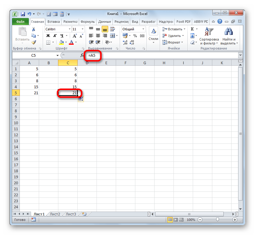
Простейшее ссылочное выражение выглядит таким образом:

=A1

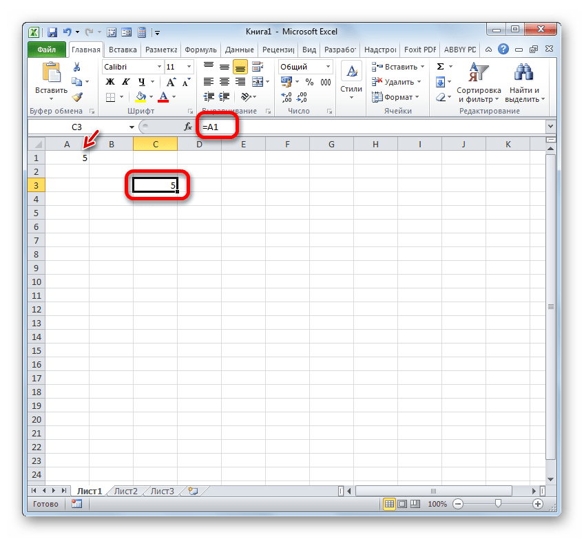
Обязательным атрибутом выражения является знак «=». Только при установке данного символа в ячейку перед выражением, оно будет восприниматься, как ссылающееся. Обязательным атрибутом также является наименование столбца (в данном случае A) и номер столбца (в данном случае 1).

Выражение «=A1» говорит о том, что в тот элемент, в котором оно установлено, подтягиваются данные из объекта с координатами A1.

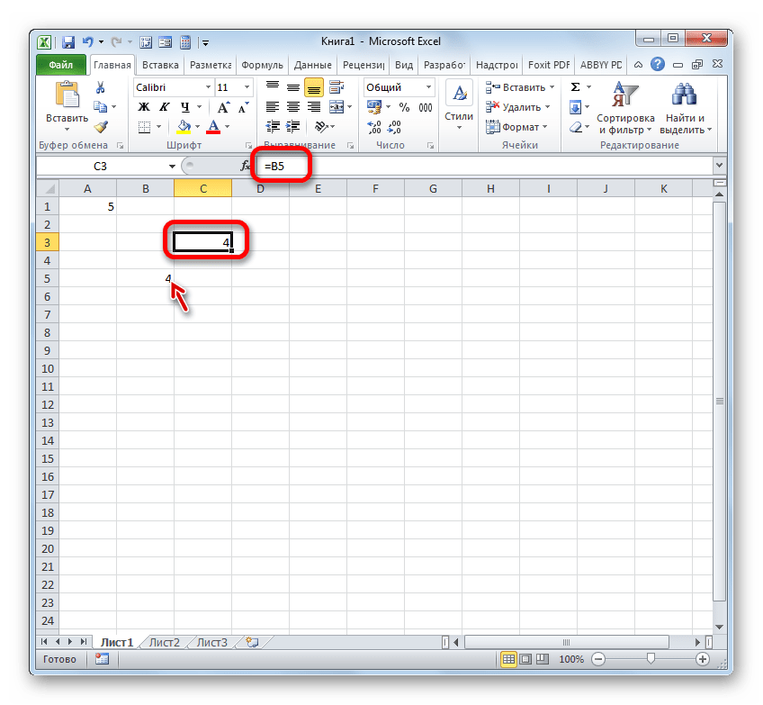
Если мы заменим выражение в ячейке, где выводится результат, например, на «=B5», то в неё будет подтягиваться значения из объекта с координатами B5.

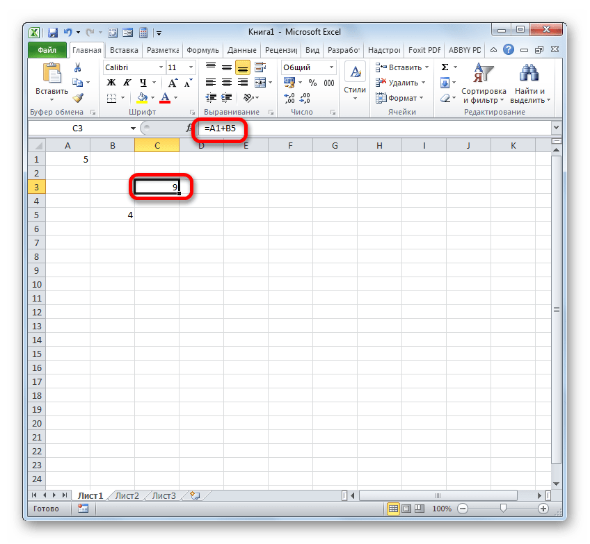
С помощью линков можно производить также различные математические действия. Например, запишем следующее выражение:

=A1+B5

Клацнем по кнопке Enter. Теперь, в том элементе, где расположено данное выражение, будет производиться суммирование значений, которые размещены в объектах с координатами A1 и B5.

По такому же принципу производится деление, умножение, вычитание и любое другое математическое действие.

Чтобы записать отдельную ссылку или в составе формулы, совсем не обязательно вбивать её с клавиатуры. Достаточно установить символ «=», а потом клацнуть левой кнопкой мыши по тому объекту, на который вы желаете сослаться. Его адрес отобразится в том объекте, где установлен знак «равно».

Но следует заметить, что стиль координат A1 не единственный, который можно применять в формулах. Параллельно в Экселе работает стиль R1C1, при котором, в отличие от предыдущего варианта, координаты обозначаются не буквами и цифрами, а исключительно числами.

Выражение R1C1 равнозначно A1, а R5C2 – B5. То есть, в данном случае, в отличие от стиля A1, на первом месте стоят координаты строки, а столбца – на втором.

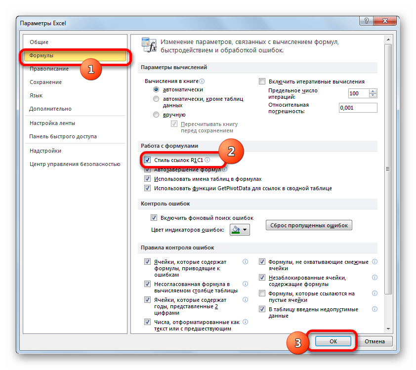
Оба стиля действуют в Excel равнозначно, но шкала координат по умолчанию имеет вид A1. Чтобы её переключить на вид R1C1 требуется в параметрах Excel в разделе «Формулы» установить флажок напротив пункта «Стиль ссылок R1C1».

После этого на горизонтальной панели координат вместо букв появятся цифры, а выражения в строке формул приобретут вид R1C1. Причем, выражения, записанные не путем внесения координат вручную, а кликом по соответствующему объекту, будут показаны в виде модуля относительно той ячейке, в которой установлены. На изображении ниже это формула

=R[2]C[-1]

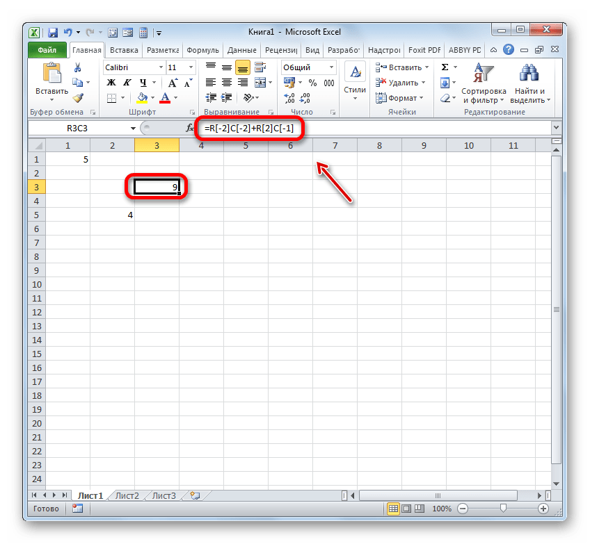
Если же записать выражение вручную, то оно примет обычный вид R1C1.

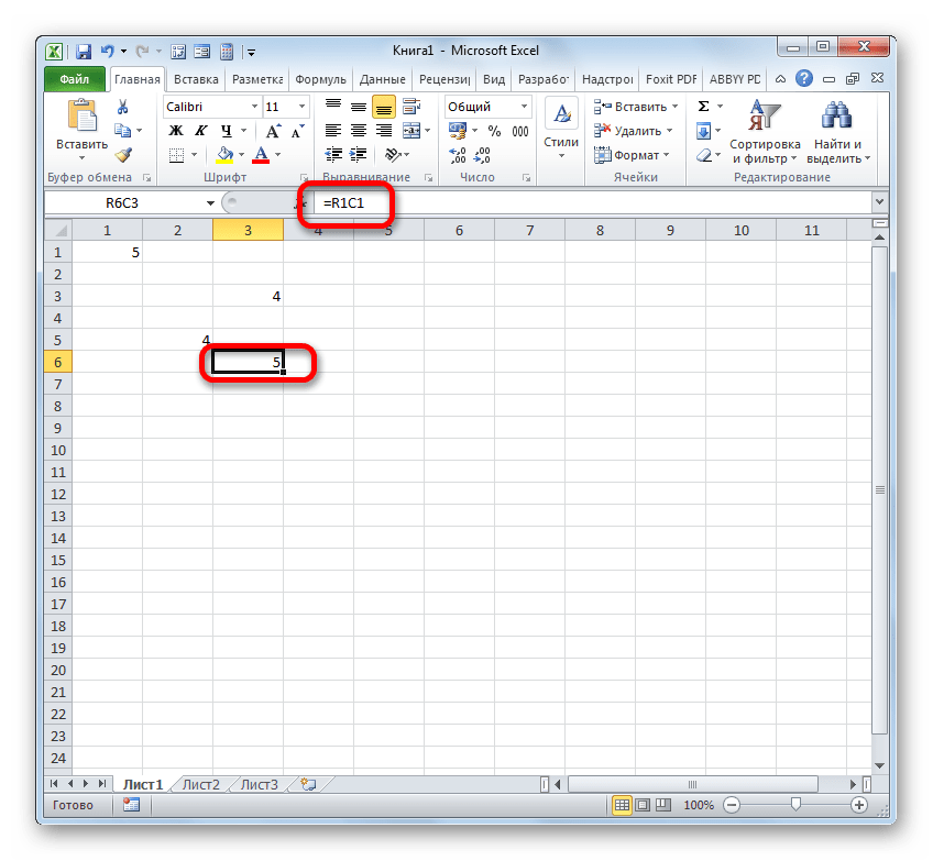
В первом случае был представлен относительный тип (=R[2]C[-1]), а во втором (=R1C1) – абсолютный. Абсолютные линки ссылаются на конкретный объект, а относительные – на положение элемента, относительно ячейки.

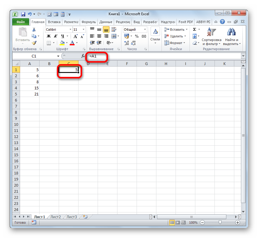
Если вернутся к стандартному стилю, то относительные линки имеют вид A1, а абсолютные $A$1. По умолчанию все ссылки, созданные в Excel, относительные. Это выражается в том, что при копировании с помощью маркера заполнения значение в них изменяется относительно перемещения.

Чтобы посмотреть, как это будет выглядеть на практике, сошлемся на ячейку A1. Устанавливаем в любом пустом элементе листа символ «=» и клацаем по объекту с координатами A1. После того, как адрес отобразился в составе формулы, клацаем по кнопке Enter.

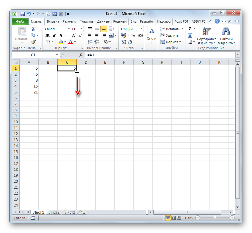
Наводим курсор на нижний правый край объекта, в котором отобразился результат обработки формулы. Курсор трансформируется в маркер заполнения. Зажимаем левую кнопку мыши и протягиваем указатель параллельно диапазону с данными, которые требуется скопировать.

После того, как копирование было завершено, мы видим, что значения в последующих элементах диапазона отличаются от того, который был в первом (копируемом) элементе. Если выделить любую ячейку, куда мы скопировали данные, то в строке формул можно увидеть, что и линк был изменен относительно перемещения. Это и есть признак его относительности.

Свойство относительности иногда очень помогает при работе с формулами и таблицами, но в некоторых случаях нужно скопировать точную формулу без изменений. Чтобы это сделать, ссылку требуется преобразовать в абсолютную.

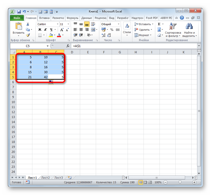
Чтобы провести преобразование, достаточно около координат по горизонтали и вертикали поставить символ доллара ($).

После того, как мы применим маркер заполнения, можно увидеть, что значение во всех последующих ячейках при копировании отображается точно такое же, как и в первой. Кроме того, при наведении на любой объект из диапазона ниже в строке формул можно заметить, что линки осталась абсолютно неизменными.

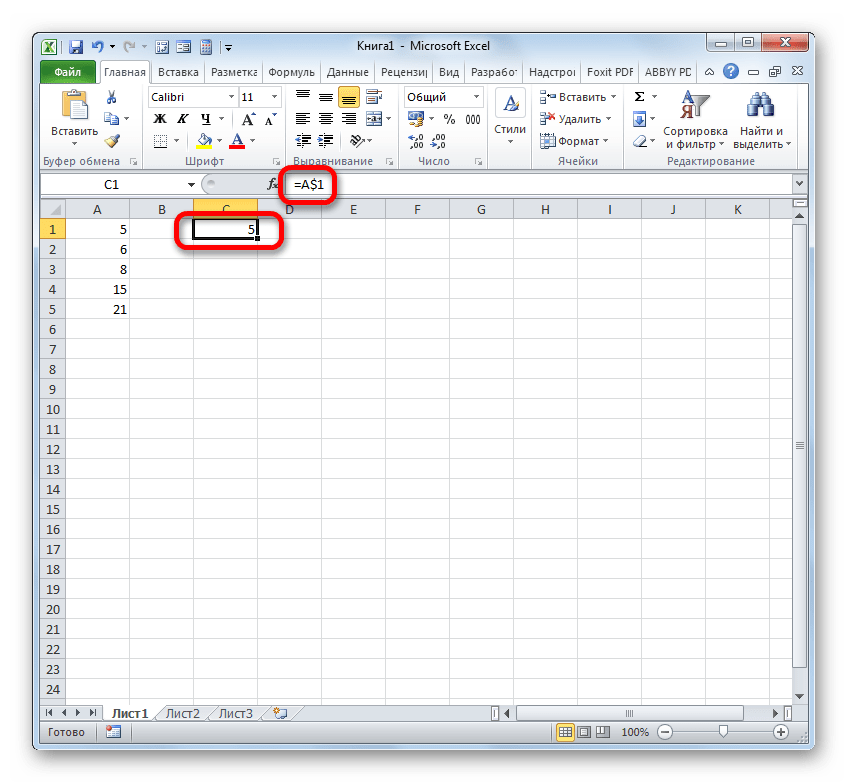
Кроме абсолютных и относительных, существуют ещё смешанные линки. В них знаком доллара отмечены либо только координаты столбца (пример: $A1),

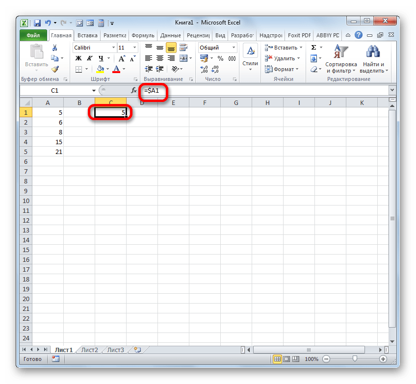
либо только координаты строки (пример: A$1).

Знак доллара можно вносить вручную, нажав на соответствующий символ на клавиатуре ($). Он будет высвечен, если в английской раскладке клавиатуры в верхнем регистре кликнуть на клавишу «4».

Но есть более удобный способ добавления указанного символа. Нужно просто выделить ссылочное выражение и нажать на клавишу F4. После этого знак доллара появится одновременно у всех координат по горизонтали и вертикали. После повторного нажатия на F4 ссылка преобразуется в смешанную: знак доллара останется только у координат строки, а у координат столбца пропадет. Ещё одно нажатие F4 приведет к обратному эффекту: знак доллара появится у координат столбцов, но пропадет у координат строк. Далее при нажатии F4 ссылка преобразуется в относительную без знаков долларов. Следующее нажатие превращает её в абсолютную. И так по новому кругу.

В Excel сослаться можно не только на конкретную ячейку, но и на целый диапазон. Адрес диапазона выглядит как координаты верхнего левого его элемента и нижнего правого, разделенные знаком двоеточия (:). К примеру, диапазон, выделенный на изображении ниже, имеет координаты A1:C5.

Соответственно линк на данный массив будет выглядеть как:

=A1:C5

Урок: Абсолютные и относительные ссылки в Майкрософт Эксель

Способ 2: создание ссылок в составе формул на другие листы и книги

До этого мы рассматривали действия только в пределах одного листа. Теперь посмотрим, как сослаться на место на другом листе или даже книге. В последнем случае это будет уже не внутренняя, а внешняя ссылка.

Принципы создания точно такие же, как мы рассматривали выше при действиях на одном листе. Только в данном случае нужно будет указать дополнительно адрес листа или книги, где находится ячейка или диапазон, на которые требуется сослаться.

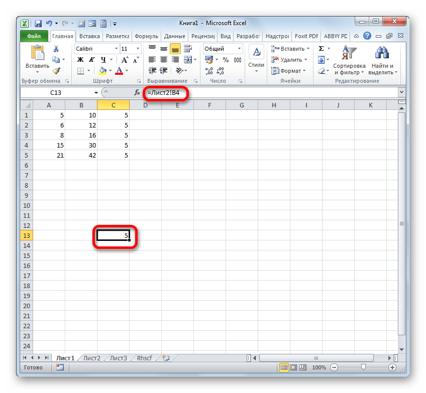
Для того, чтобы сослаться на значение на другом листе, нужно между знаком «=» и координатами ячейки указать его название, после чего установить восклицательный знак.

Так линк на ячейку на Листе 2 с координатами B4 будет выглядеть следующим образом:

=Лист2!B4

Выражение можно вбить вручную с клавиатуры, но гораздо удобнее поступить следующим образом.

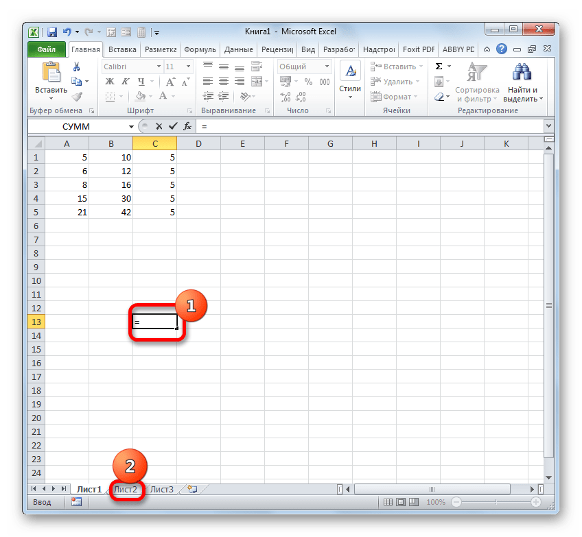
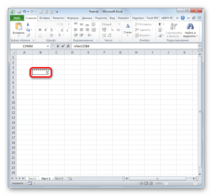
Устанавливаем знак «=» в элементе, который будет содержать ссылающееся выражение. После этого с помощью ярлыка над строкой состояния переходим на тот лист, где расположен объект, на который требуется сослаться.

После перехода выделяем данный объект (ячейку или диапазон) и жмем на кнопку Enter.

После этого произойдет автоматический возврат на предыдущий лист, но при этом будет сформирована нужная нам ссылка.

Теперь давайте разберемся, как сослаться на элемент, расположенный в другой книге. Прежде всего, нужно знать, что принципы работы различных функций и инструментов Excel с другими книгами отличаются. Некоторые из них работают с другими файлами Excel, даже когда те закрыты, а другие для взаимодействия требуют обязательного запуска этих файлов.

В связи с этими особенностями отличается и вид линка на другие книги. Если вы внедряете его в инструмент, работающий исключительно с запущенными файлами, то в этом случае можно просто указать наименование книги, на которую вы ссылаетесь. Если же вы предполагаете работать с файлом, который не собираетесь открывать, то в этом случае нужно указать полный путь к нему. Если вы не знаете, в каком режиме будете работать с файлом или не уверены, как с ним может работать конкретный инструмент, то в этом случае опять же лучше указать полный путь. Лишним это точно не будет.

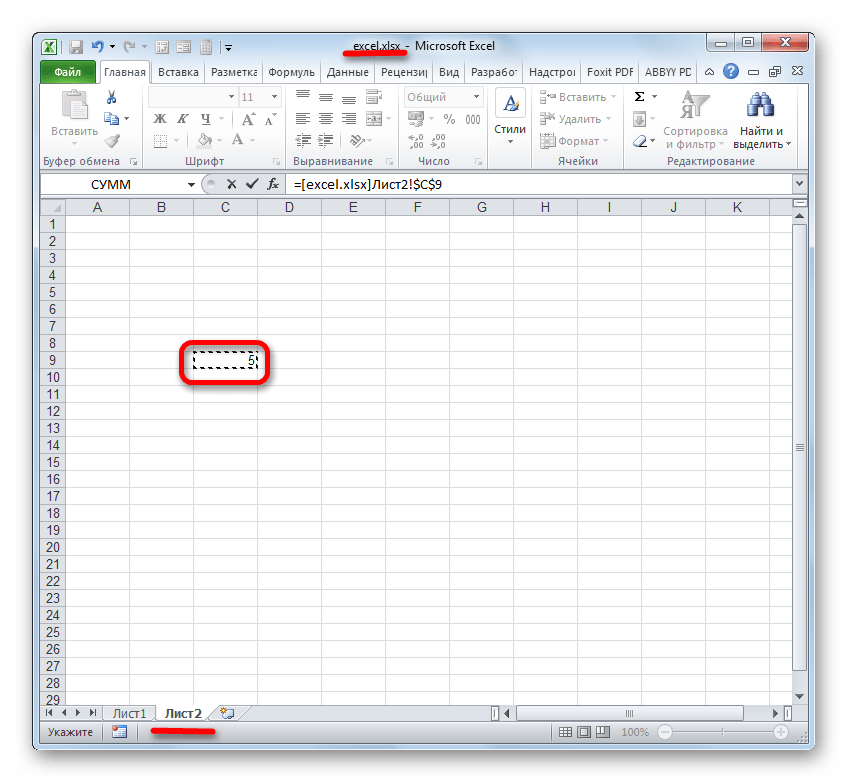
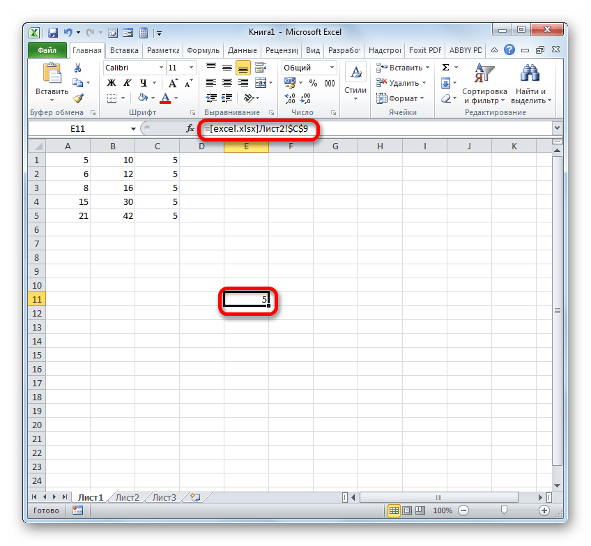
Если нужно сослаться на объект с адресом C9, расположенный на Листе 2 в запущенной книге под названием «Excel.xlsx», то следует записать следующее выражение в элемент листа, куда будет выводиться значение:

=[excel.xlsx]Лист2!C9

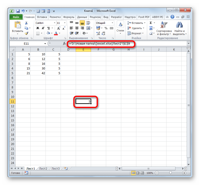
Если же вы планируете работать с закрытым документом, то кроме всего прочего нужно указать и путь его расположения. Например:

='D:Новая папка[excel.xlsx]Лист2'!C9

Как и в случае создания ссылающегося выражения на другой лист, при создании линка на элемент другой книги можно, как ввести его вручную, так и сделать это путем выделения соответствующей ячейки или диапазона в другом файле.

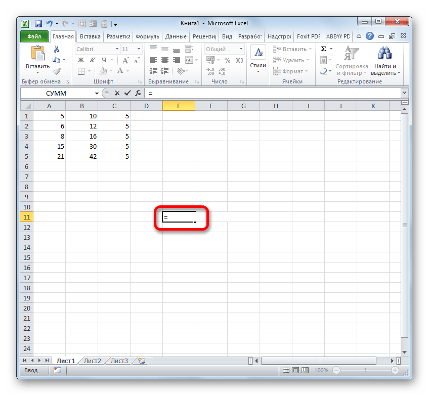
Ставим символ «=» в той ячейке, где будет расположено ссылающееся выражение.

Затем открываем книгу, на которую требуется сослаться, если она не запущена. Клацаем на её листе в том месте, на которое требуется сослаться. После этого кликаем по Enter.

Происходит автоматический возврат к предыдущей книге. Как видим, в ней уже проставлен линк на элемент того файла, по которому мы щелкнули на предыдущем шаге. Он содержит только наименование без пути.

Но если мы закроем файл, на который ссылаемся, линк тут же преобразится автоматически. В нем будет представлен полный путь к файлу. Таким образом, если формула, функция или инструмент поддерживает работу с закрытыми книгами, то теперь, благодаря трансформации ссылающегося выражения, можно будет воспользоваться этой возможностью.

Как видим, проставление ссылки на элемент другого файла с помощью клика по нему не только намного удобнее, чем вписывание адреса вручную, но и более универсальное, так как в таком случае линк сам трансформируется в зависимости от того, закрыта книга, на которую он ссылается, или открыта.

Способ 3: функция ДВССЫЛ

Ещё одним вариантом сослаться на объект в Экселе является применение функции ДВССЫЛ. Данный инструмент как раз и предназначен именно для того, чтобы создавать ссылочные выражения в текстовом виде. Созданные таким образом ссылки ещё называют «суперабсолютными», так как они связаны с указанной в них ячейкой ещё более крепко, чем типичные абсолютные выражения. Синтаксис этого оператора:

=ДВССЫЛ(ссылка;a1)

«Ссылка» — это аргумент, ссылающийся на ячейку в текстовом виде (обернут кавычками);

«A1» — необязательный аргумент, который определяет, в каком стиле используются координаты: A1 или R1C1. Если значение данного аргумента «ИСТИНА», то применяется первый вариант, если «ЛОЖЬ» — то второй. Если данный аргумент вообще опустить, то по умолчанию считается, что применяются адресация типа A1.

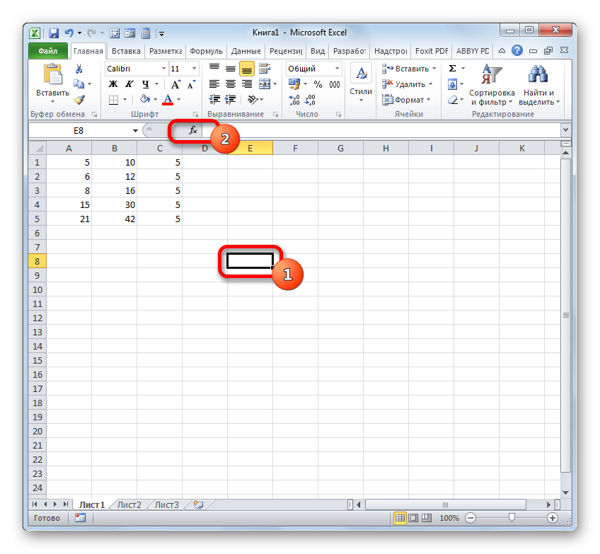
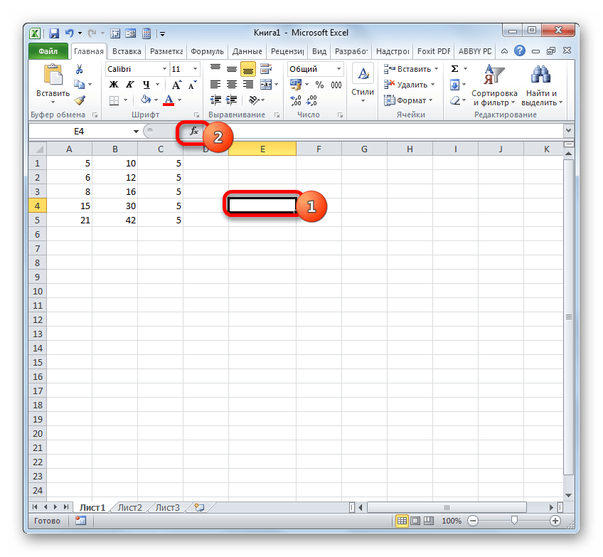
Отмечаем элемент листа, в котором будет находиться формула. Клацаем по пиктограмме «Вставить функцию».

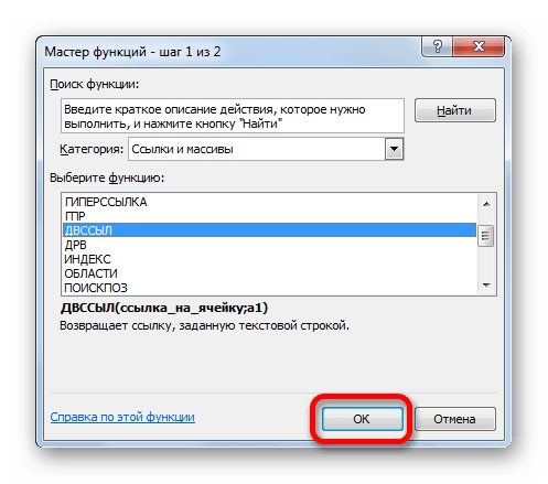
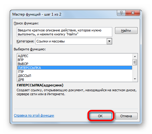
В Мастере функций в блоке «Ссылки и массивы» отмечаем «ДВССЫЛ». Жмем «OK».

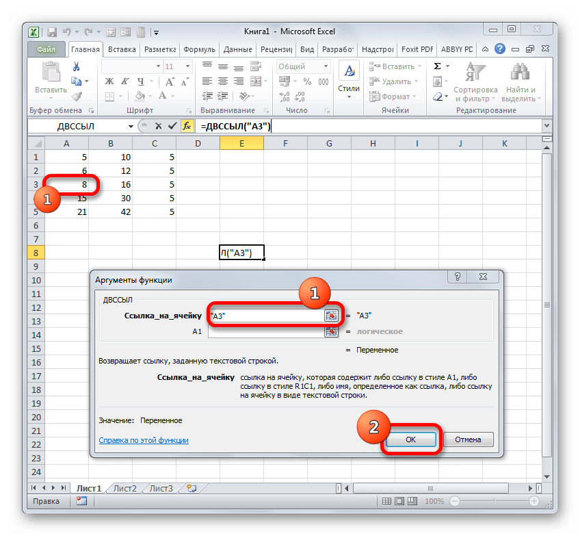
Открывается окно аргументов данного оператора. В поле «Ссылка на ячейку» устанавливаем курсор и выделяем кликом мышки тот элемент на листе, на который желаем сослаться. После того, как адрес отобразился в поле, «оборачиваем» его кавычками. Второе поле («A1») оставляем пустым. Кликаем по «OK».

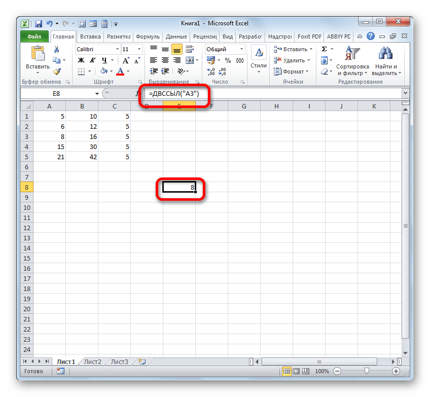
Результат обработки данной функции отображается в выделенной ячейке.

Более подробно преимущества и нюансы работы с функцией ДВССЫЛ рассмотрены в отдельном уроке.

Урок: Функция ДВССЫЛ в Майкрософт Эксель

Способ 4: создание гиперссылок

Гиперссылки отличаются от того типа ссылок, который мы рассматривали выше. Они служат не для того, чтобы «подтягивать» данные из других областей в ту ячейку, где они расположены, а для того, чтобы совершать переход при клике в ту область, на которую они ссылаются.

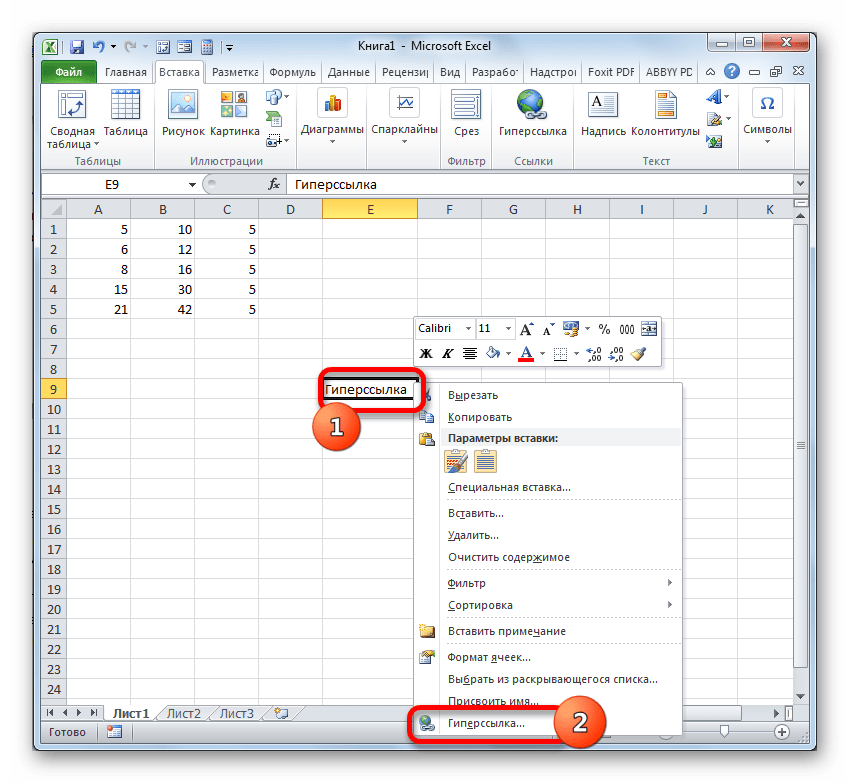
Существует три варианта перехода к окну создания гиперссылок. Согласно первому из них, нужно выделить ячейку, в которую будет вставлена гиперссылка, и кликнуть по ней правой кнопкой мыши. В контекстном меню выбираем вариант «Гиперссылка…».

Вместо этого можно, после выделения элемента, куда будет вставлена гиперссылка, перейти во вкладку «Вставка». Там на ленте требуется щелкнуть по кнопке «Гиперссылка».

Также после выделения ячейки можно применить нажатие клавиш CTRL+K.
После применения любого из этих трех вариантов откроется окно создания гиперссылки. В левой части окна существует возможность выбора, с каким объектом требуется связаться:
- С местом в текущей книге;
- С новой книгой;
- С веб-сайтом или файлом;
- С e-mail.

По умолчанию окно запускается в режиме связи с файлом или веб-страницей. Для того, чтобы связать элемент с файлом, в центральной части окна с помощью инструментов навигации требуется перейти в ту директорию жесткого диска, где расположен нужный файл, и выделить его. Это может быть как книга Excel, так и файл любого другого формата. После этого координаты отобразятся в поле «Адрес». Далее для завершения операции следует нажать на кнопку «OK».

Если имеется потребность произвести связь с веб-сайтом, то в этом случае в том же разделе окна создания гиперссылки в поле «Адрес» нужно просто указать адрес нужного веб-ресурса и нажать на кнопку «OK».

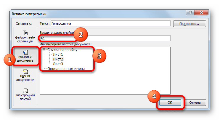
Если требуется указать гиперссылку на место в текущей книге, то следует перейти в раздел «Связать с местом в документе». Далее в центральной части окна нужно указать лист и адрес той ячейки, с которой следует произвести связь. Кликаем по «OK».

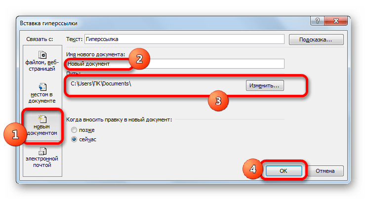
Если нужно создать новый документ Excel и привязать его с помощью гиперссылки к текущей книге, то следует перейти в раздел «Связать с новым документом». Далее в центральной области окна дать ему имя и указать его местоположение на диске. Затем кликнуть по «OK».

При желании можно связать элемент листа гиперссылкой даже с электронной почтой. Для этого перемещаемся в раздел «Связать с электронной почтой» и в поле «Адрес» указываем e-mail. Клацаем по «OK».

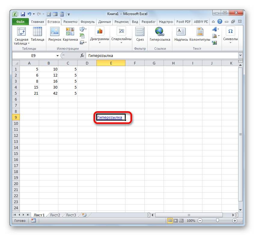
После того, как гиперссылка была вставлена, текст в той ячейке, в которой она расположена, по умолчанию приобретает синий цвет. Это значит, что гиперссылка активна. Чтобы перейти к тому объекту, с которым она связана, достаточно выполнить двойной щелчок по ней левой кнопкой мыши.

Кроме того, гиперссылку можно сгенерировать с помощью встроенной функции, имеющей название, которое говорит само за себя – «ГИПЕРССЫЛКА».

Данный оператор имеет синтаксис:

=ГИПЕРССЫЛКА(адрес;имя)

«Адрес» — аргумент, указывающий адрес веб-сайта в интернете или файла на винчестере, с которым нужно установить связь.

«Имя» — аргумент в виде текста, который будет отображаться в элементе листа, содержащем гиперссылку. Этот аргумент не является обязательным. При его отсутствии в элементе листа будет отображаться адрес объекта, на который функция ссылается.

Выделяем ячейку, в которой будет размещаться гиперссылка, и клацаем по иконке «Вставить функцию».

В Мастере функций переходим в раздел «Ссылки и массивы». Отмечаем название «ГИПЕРССЫЛКА» и кликаем по «OK».

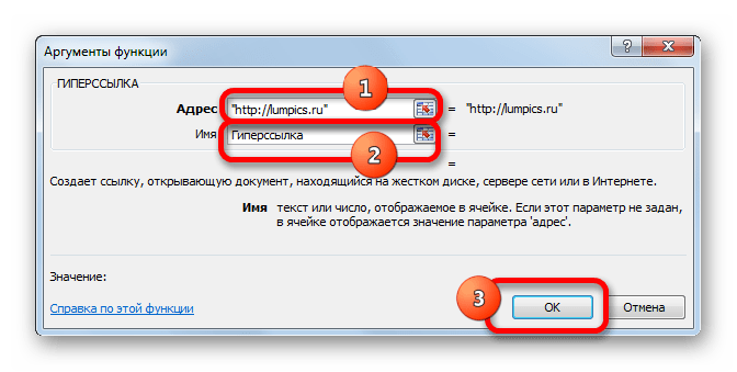
В окне аргументов в поле «Адрес» указываем адрес на веб-сайт или файл на винчестере. В поле «Имя» пишем текст, который будет отображаться в элементе листа. Клацаем по «OK».

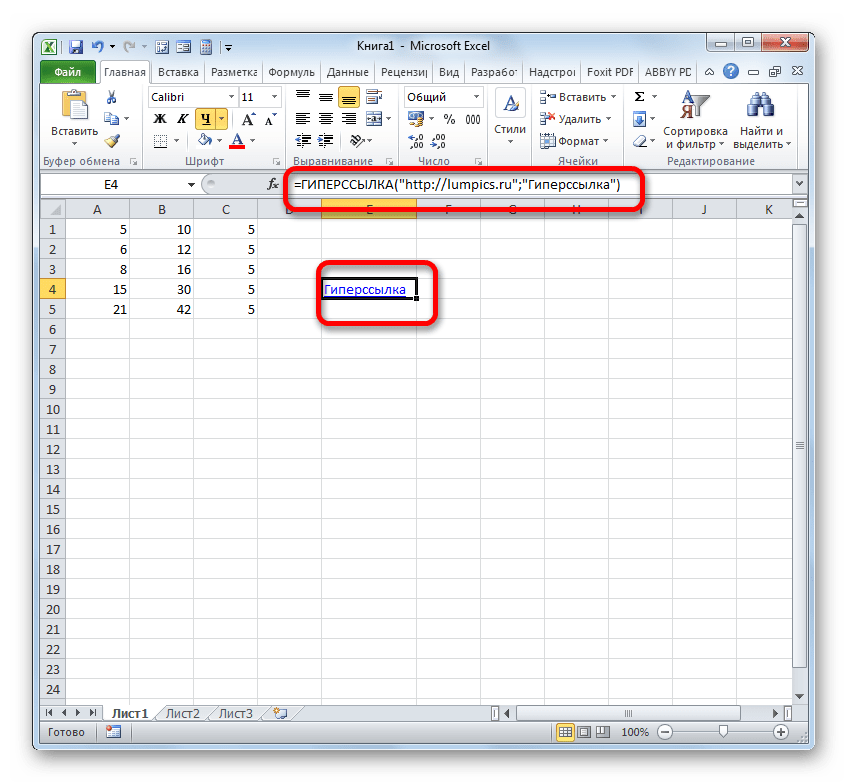
После этого гиперссылка будет создана.

Урок: Как сделать или удалить гиперссылки в Экселе

Мы выяснили, что в таблицах Excel существует две группы ссылок: применяющиеся в формулах и служащие для перехода (гиперссылки). Кроме того, эти две группы делятся на множество более мелких разновидностей. Именно от конкретной разновидности линка и зависит алгоритм процедуры создания.

Источник

Excel files are also called workbooks for a very good reason. They can have multiple sheets, or worksheets, to help you organize your data. When working with multiple sheets, you may need to have links between them so that values in one sheet can be used in another.

In this article, we’ll explain how to link data between worksheets in Excel. You’ll see several examples on linking sheets in the same workbook as well as across different ones.

Why link data between sheets in Excel?

Linking sheets in Excel can be a great way to organize your data and keep them consistent across different worksheets. You may want to do this for different purposes, for example:

You have a workbook containing data split by month, by state, or by salesperson, and you want a summary in one of the sheets.
You want to create lists using links from different sheets in Excel.
You want to collect data from multiple sheets and combine them into one to create a master sheet. Or, you may want to link data from a master sheet so that your data in other sheets are always up-to-date.
Your data is growing and becoming too voluminous. As a result, you split it into different workbooks to be managed by different people. There can be times when you need to write formulas to get data out of these files.

Creating links between sheets is pretty easy to do. Besides, the main benefit is that whenever your data in the source sheet changes, the data in the destination sheet will be automatically updated as well.

Problems with linking large data between worksheets in the same or different Excel workbooks

Indeed, using multiple worksheets can certainly make your data in one workbook easier to manage. However, linking large amounts of data between worksheets could decrease the performance of your Excel workbook. Avoid inter-workbook links unless it’s absolutely necessary because they can be slow, easily broken, and not always easy to find and fix.

We suggest you try another solution 👇

When getting large data from different worksheets, especially from different workbooks, we recommend that you import instead of linking. Linking will slow down your Excel file, while an optimized performance can be maintained if you simply import data from Excel to Excel. Use a tool such as Coupler.io to refresh your data on the schedule you want to keep your data up-to-date.

To start using Coupler.io, sign up for a free account and create your first importer. A wizard will walk you through setting up the source, destination, and auto-refresh schedule for your importer. If you’re importing from Excel to Excel, choose Microsoft Excel as the source and destination of your importer, as follows:

#1. Set up a source

Select Microsoft Excel as the source that contains your data. You’ll need to connect to your Microsoft account and select the workbook and worksheet(s) you want to import. If you want, you can import only a selected range from your worksheets, e.g., range B3:G10 only.

Notice that with Coupler.io, you can also import data from different sources such as HubSpot, Jira, QuickBooks, and more. Check out the complete list of Coupler.io integrations with Excel.

#2. Set up a destination

For the destination, select Microsoft Excel. No need to connect again if you’re importing to the same Microsoft account. After that, choose the workbook and worksheet where you want your data imported.

#3. Schedule

You can keep your data up-to-date by setting up an automatic data refresh on the schedule you want.

Finally, click Save and Run to run your first importer. The import process may take several seconds or minutes to complete.

How to link two Excel sheets in the same workbook

Now, let’s see how to link two sheets in the same Excel workbook, including some tips and examples.

How to link sheets in Excel with a formula

To refer to a cell or range in another worksheet in the same workbook, type the name of the source worksheet followed by an exclamation mark (!) before the range address—see the following examples:

To reference a single cell A1 in Sheet2:

=Sheet2!A1

To reference a single cell A1 but the sheet name contains spaces:

='Sheet 2'!A1

To reference a range of cells A1 to C10 in Sheet2:

=Sheet2!A1:C10

To reference column A in Sheet2:

=Sheet2!A:A

To reference multiple columns A to E in Sheet2:

=Sheet2!A:E

To reference row 5 in Sheet2:

=Sheet2!5:5

To reference multiple rows 1 to 5 in Sheet2:

=Sheet2!1:5

To reference a worksheet-level named range Data in Sheet2:

=Sheet2!Data

To reference a workbook-level named range Data in Sheet2:

=Data

You can always manually type the linking formula in a destination cell. However, doing that is not recommended because it typically leads to mistakes. So, instead of typing the formula manually, check the tips below.

Tip 1: Create a link from the destination sheet

With the following spreadsheet, suppose you want to show the total for New York in the Summary sheet. In cell B2 of the Summary sheet, you want to display the values of cell F5 from the New York sheet.

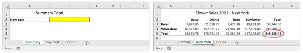
To do that, follow the steps below:

Begin by opening the destination sheet (Summary).
Type = (equal sign) in the destination cell (B2).

Switch to source sheet (New York).
Select the cell you want to link (F5), then press Enter.

As a result, when you click on the destination cell, you’ll see the following formula:

='New York'!F5

Notice that Excel automatically encloses the sheet name with single quotation marks because there is a space character in the sheet name.

Tip 2: Use Copy and Paste Link

This second tip also allows you to link to another sheet without manually typing the linking formula. Unlike the first method that begins from the destination sheet, this method starts from the source sheet.

This time, suppose you want to show the total for Florida in the Summary sheet. In cell B3 of the Summary sheet, you want to display the values of cell F5 from the Florida sheet.

Follow the steps below:

Begin by opening the source sheet (Florida).
Right-click on the cell you want to link (F5), then select Copy.

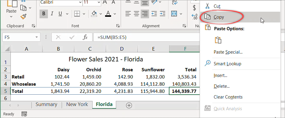
Switch to the destination sheet (Summary).
In the destination cell (B3), right-click and select Paste Link.

As a result, when you click on B3, you’ll see the following formula:

=Florida!$F$5

Notice that by default, this method returns an absolute reference. If you want to change it to a relative reference, simply highlight the formula and press F4 multiple times to remove the dollar signs.

How to link numbers from different sheets in Excel using the INDIRECT function

In the previous example, notice that the New York and Florida sheets have the same layout. In cases like this, you can also use the INDIRECT function in the formula to get the totals.

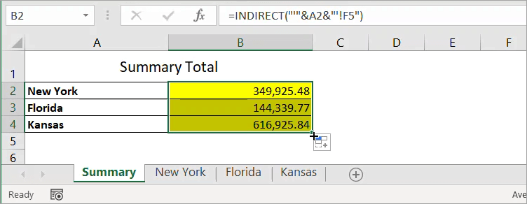
Now, let’s see the following spreadsheet with a Summary sheet and three other sheets with a similar layout. Assume you want to link the total in cell F5 from the three sheets and put them in the Summary sheet using the INDIRECT function.

To do that, follow the steps below:

Link the total for New York only:

='New York'!F5

Replace the formula using the INDIRECT function below. Notice that we concatenate A2 with single quotes because its value contains a space character.

=INDIRECT("'"&A2&"'!F5")

Drag the formula down to A4 to apply it to the other states.

How to link data in a range of cells between sheets in Excel

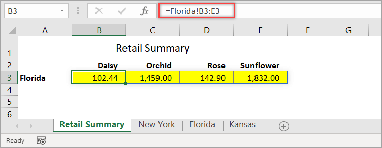
With the following spreadsheet, suppose you want to link the retail sales data for Florida and put them in the Retail Summary sheet, as the following screenshot shows:

The range to link is in B3:E3 of the second sheet. To display it in the destination sheet, use the following formula in a cell:

=Florida!B3:E3

How to link columns from different sheets to another sheet in Excel

With the following spreadsheet, suppose you want to link the entire Column B from the Product sheet to Sheet1. To do that, you can use the following formula:

=Product!B:B

However, if you notice, the blank cells are showing zeros. If you want to see empty cells when there is nothing in the original sheet, you can change the formula to the one below:

=IF(LEN(Product!B:B)>0, Product!B:B,"")

How to link to a defined name in other sheets in Excel

For most people, words are easier to remember than numbers or codes. For this reason, Excel allows you to name an individual cell or range of cells. Then, you can use these names when referring to data in another sheet instead of typing the range address.

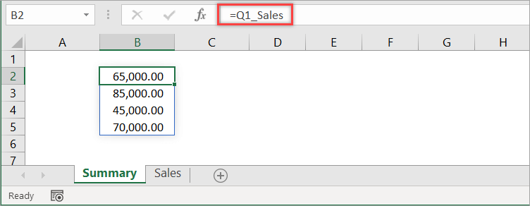
With the following worksheet, let’s create a defined name for range B2:B5 and name it Q1_Sales.

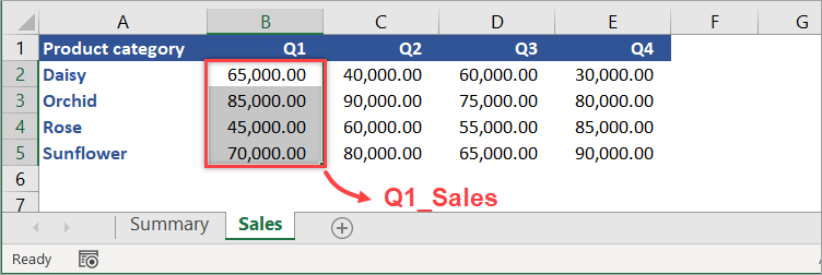
First, select the range of cells to include (B2:B5). Then, in the Name Box, type Q1_Sales and press Enter — and Done!

By default, Excel creates the name at the workbook level. To reference the defined name in another worksheet, just type the following formula into any cell.

=Q1_Sales

You can also use the defined name with an Excel function in a formula. For example, the following formula calculates the average of Q1_Sales:

=AVERAGE(Q1_Sales)

How to link lists in different sheets in Excel

With the following spreadsheet, suppose you want to create a dropdown list in Sheet1 that contains product category data from Sheet2. This will allow you to select the Category in Column D using a dropdown instead of typing it manually.

Follow these steps:

In Sheet1, select the range you want to apply to the dropdown list, which is D2:D4.
Click Data > Data Validation.
In the “Data Validation” dialog box, enter the following details, then click OK.

Allow : List
Source : =Sheet2!$A$2:$A$5

We enter a link reference to product category data in Sheet2, which is in range A2:A5. As a result, now you select the product category in Sheet1 using a dropdown, as shown below:

How to link to hidden sheets in Excel

A sheet can be hidden for different reasons. For example, you may want to hide sheets that are no longer frequently being used by other users.

To create a link to a hidden sheet, simply unhide it first, create the link, then hide it again if necessary.

You can actually refer to hidden sheets without unhiding them first, as long as you know the name of the sheets and the range you want to link from these sheets. However, most of the time, you’ll need to unhide them first to see the data you want to link so that you don’t accidentally refer to the wrong range of cells when creating the links.

There are two different types of hidden sheets in Excel: hidden and very hidden. While unhiding a hidden sheet is very easy, you will need to open the Visual Basic Editor (VBE) to unhide a very hidden sheet.

To link to a hidden sheet in Excel

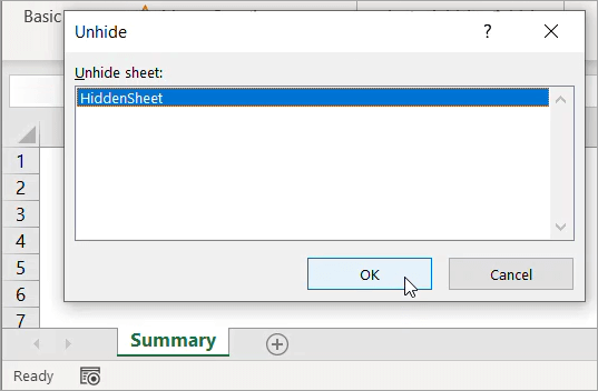
Unhide the sheet by right-clicking on any visible sheet, then select Unhide.

In the “Unhide” dialog box that appears, select the sheet you want to unhide, then click OK.

Use a linking formula to link the data you want to show in another sheet.
For example, the following formula in the Summary sheet shows the range A1:E1 from the sheet we just made visible.

=HiddenSheet!A1:E1

If you want, hide the sheet again by clicking on the sheet tab, then select Hide.

To link to a very hidden sheet in Excel

Open the VBE by pressing Alt+F11.
Press F4 or click View > Properties Window to open the Properties window under the Project Explorer if it’s not already open.
In Project Explorer, select the very hidden sheet you want to unhide. Then, set its Visible property to -1 - xlSheetVisible in the Properties window.

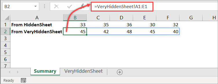
Use a linking formula to link the data you want to show in another sheet. For example, the following formula in the Summary sheet shows the range A1:E1 from the very hidden sheet we just made visible.

=VeryHiddenSheet!A1:E1

If you want, change the sheet’s Visible property back to 2 - xlSheetVeryHidden in the Properties window to make it a very hidden sheet again.

How to link sheets in Excel to a master sheet

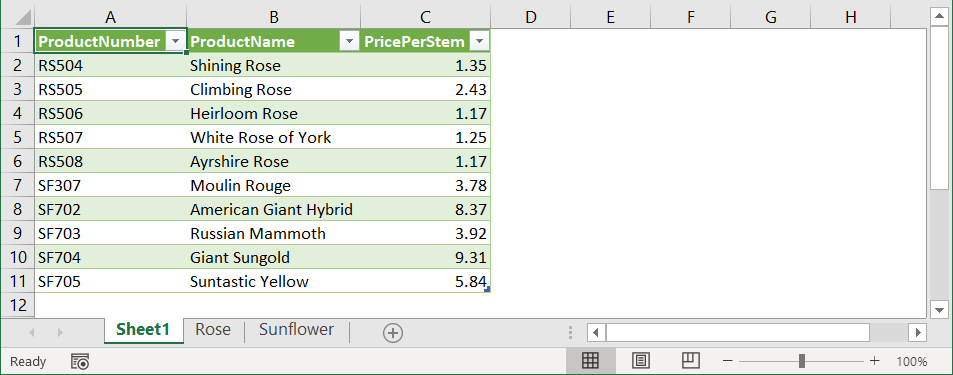
With the following spreadsheet, suppose you want to link data from two worksheets into one.

Notice that it’s like combining two ranges, which are Rose!A1:C6 and Sunflower!A1:C6.

However, combining ranges in Excel using a formula is a bit complex. An easier way to do this is using Power Query, as explained in the steps below:

In the Rose sheet, select the range A1:C6.
Then, on the Data tab in the Get & Transform Data section, click From Table/Range.
In the “Create Table” dialog box, ensure that the My table has headers option checked.

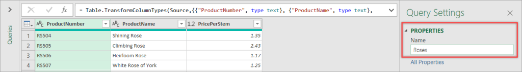
Click OK — this will bring you to the Power Query editor.
In the Query Settings, give your query a descriptive name, e.g., Roses.

Click the Home tab, then click Close & Load > Close & Load To…
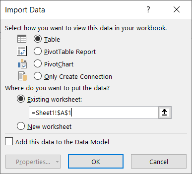
In the “Import Data” dialog box, select Only Create Connection, then press OK.

Repeat steps 1-7 for the Sunflower data. But for the fifth step, let’s rename the query as Sunflowers.
Re-launch the Power Query editor by clicking the Data tab, then click Get Data > Launch Power Query Editor…
Select any query, then click Append Queries > Append Queries as New to keep the existing queries unchanged.

In the Append window, select the other table as the second table, then click OK.

Make sure to select the newly created query. Then, on the Home tab, click Close & Load > Close & Load To…
In the “Import Data” dialog box, load the combined data to Sheet1!A1, then click OK.

To see the result, click Sheet1. You’ll find the combined data as shown in the following screenshot:

When the source data from the other sheets change, you won’t see the new changes right away. Using this method, you need to click the Refresh All button in the Data tab to see the latest data.

How to link two Excel sheets in different workbooks

To link to a worksheet in another workbook, you can do it whether the source file is open or closed. If possible, we suggest you open all the source workbooks first before creating the links in the destination workbook. Why? Because this way is easier.

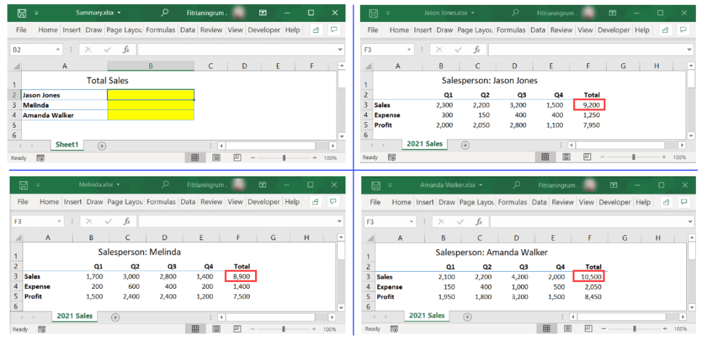
As an example, suppose you have the following four workbooks: Summary.xlsx, Jason Jones.xlsx, Melinda.xlsx, and Amanda Walker.xlsx. In the Summary workbook, you want to link the total sales of each salesperson, which is in cell F3 of each of the other workbooks—see the following screenshot:

Link to another worksheet when the source workbook is open

When all the source files are open, you can follow the steps below to create the links:

In the Summary workbook, type = (equal sign) in the destination cell for Jason Jones.

Click View > Switch Windows, then select Jason Jones.xlsx to switch to this workbook.

Select the cell to link, in this case, F3, then press Enter.

Repeat Steps 1-3 for Melinda and Amanda Walker.

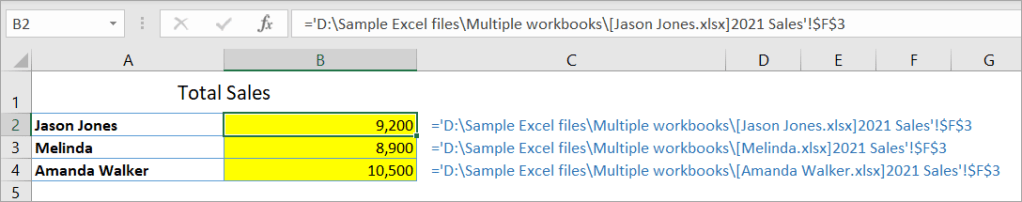
As the final result, you’ll see formulas with the following format when you click on each of the destination cells:

='[SourceWorkbook.xlsx]SheetName'!RangeAddress

Note: In the above example, the workbook name and/or sheet name contain spaces, so the path is enclosed in single quotation marks.

Link to another worksheet when the source workbook is closed

If you close the source workbooks one by one, the linking formulas in the Summary workbook will change as shown in the below screenshot:

Now, you get the idea — you need to use the full path when linking to a workbook that’s currently closed.

Basically, you can use the following format to link data from any Excel workbooks:

='FolderPath[SourceWorkbook.xlsx]SheetName'!RangeAddress

However, if possible, just open the source files before you create the link, so you don’t need to manually type the long formula that’s shown above. 🙂

Can you break links between sheets in different workbooks in Excel?

When you open an Excel file, there may be formulas in it that get data from another workbook.

To locate these formulas, click on the Data tab in the ribbon. If the Edit Links button is available, it means that your file contains links to other workbooks.

To break a link, follow these steps:

On the Data tab, in the Queries & Connections section, click Edit Links.
In the “Edit Links” dialog box that appears, select the link you want to break and click Break Link.

Click Break Links in the confirmation dialog box that appears.

Notice that when you break a link to the source workbook, all the linking formulas are converted to their current values. This action cannot be undone, so you may want to back up your workbook before breaking any links.

Click Close.

In this section, you’ve learned the basics of how to link sheets from different workbooks, as well as how to break those links. If you’re interested in more examples of linking worksheets from different workbooks, check out our article on how to link Excel files.

Thanks for reading, and good luck with your data!

Senior analyst programmer

Back to Blog

Focus on your business

goals while we take care of your data!

Try Coupler.io

Источник

See all How-To Articles

This tutorial demonstrates how to hyperlink to another sheet or workbook in Excel and Google Sheets.

Link to Another Sheet

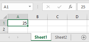
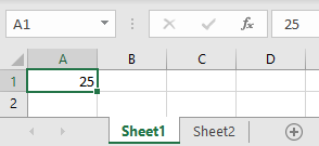
In Excel, you can create a hyperlink to a cell in another sheet. Say you have value 25 in cell A1 of Sheet1 and want to create a hyperlink to this cell in Sheet2.

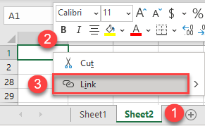
Go to another sheet (Sheet2), right-click the cell where you want to insert a hyperlink (A1), and click Link.

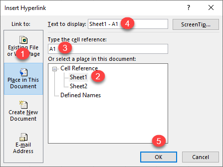
In the Insert Hyperlink window, (1) select Place in This Document, (2) choose a sheet to which you want to link (Sheet1), (3) enter the cell you want to link to (A1), (4) enter text to display in the linked cell (Sheet1 – A1), and (5) click OK.

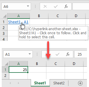
As a result, the hyperlink is inserted in cell A1 of Sheet2. By default, the text of the hyperlink is underlined and colored in blue. If you position a mouse cursor over the hyperlink, you can see the file destination and name, as well as a cell that it’s leading to.

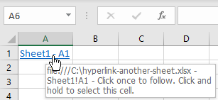
And when you click on the hyperlink, you’ll be redirected to the linked cell.

The HYPERLINK Function

Another way to insert a hyperlink to another sheet is to use the HYPERLINK Function. Enter this formula in cell A1 of Sheet2:

=HYPERLINK(Sheet1!A1,"Sheet1 - A1")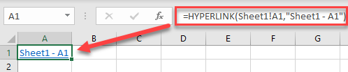

The first argument of the function is the cell to which you want to navigate the link, and the second argument is the text that is displayed in the link. The result is the same as using the previous method.

Hyperlink to Another Workbook

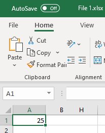
You can also insert a hyperlink to another workbook. Say that in File 1.xlsx you have a value of 25 in cell A1 and want to link it to File 2.xlsx.

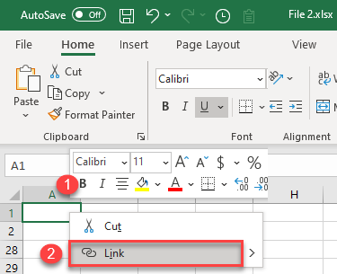
In File 2.xlsx, right-click the cell where you want to insert a hyperlink (A1) and click Link.

In the Insert Hyperlink window, (1) select Existing File or Web Page, (2) choose Current Folder – or (3) select the folder with your source file – and (4) select the file (File 1.xlsx). (5) Enter text to display in the linked cell (File 1), and (6) click OK.

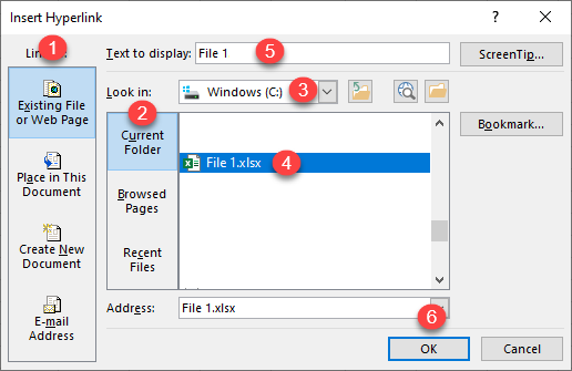
As a result, the hyperlink to File 1.xlsx is inserted into cell A1 of File 2.xlsx. If you position a mouse cursor over this cell, you can see the linked file destination and name.

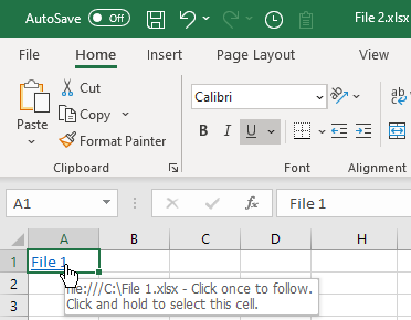
If you click on the link, you’re redirected to cell A1 of the source file. If the source file is not opened, it is opened once you click the hyperlink.

Link to Another Google Sheets Tab

To create a hyperlink to another sheet in Google Sheets, follow these steps:

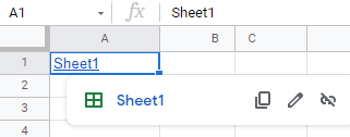
Go to another sheet (Sheet2), right-click the cell where you want to insert a hyperlink (A1), and click Insert link.

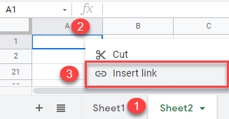
Select the sheet you want to link to (Sheet1).

As a result, the hyperlink is inserted in cell A1 of Sheet2. By default, the text of the hyperlink is underlined and colored in blue. If you click on a cell with the link, you can see the linked sheet.

And when you click on the hyperlink, you’ll be redirected to the linked sheet.

Link to Another Google Sheet

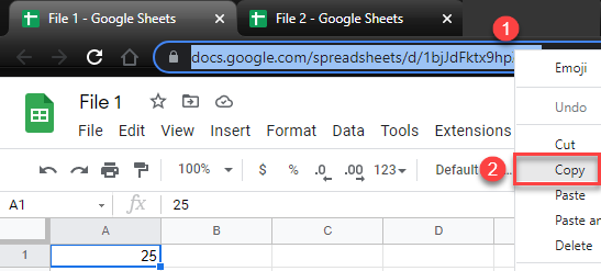
Say you have File 1 in Google Sheets with value 25 in cell A1 and want to link this cell to File 2.

Right-click the URL address of the source file (File 1) and click Copy.

Now go to another file (File 2), right-click the cell where you want to insert a hyperlink (A1), and click Insert link.

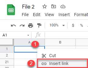
Paste the copied link, enter text to display, and click Apply.

As a result, the hyperlink is inserted in cell A1. If you click on this cell, you can navigate to the linked file (File 1).

Note: You can also use the HYPERLINK Function in Google Sheets, same as in Excel. The only difference is that for Google Sheets, you have to enter the URL.

Источник

Need more help?

See Also

Things You Should Know

Video

About This Article

Is this article up to date?

Создание различных типов ссылок

Способ 1: создание ссылок в составе формул в пределах одного листа

Способ 2: создание ссылок в составе формул на другие листы и книги

Способ 3: функция ДВССЫЛ

Способ 4: создание гиперссылок

Why link data between sheets in Excel?

Problems with linking large data between worksheets in the same or different Excel workbooks

How to link two Excel sheets in the same workbook

How to link sheets in Excel with a formula

Tip 1: Create a link from the destination sheet

Tip 2: Use Copy and Paste Link

How to link numbers from different sheets in Excel using the INDIRECT function

How to link data in a range of cells between sheets in Excel

How to link columns from different sheets to another sheet in Excel

How to link to a defined name in other sheets in Excel

How to link lists in different sheets in Excel

How to link to hidden sheets in Excel

To link to a hidden sheet in Excel

To link to a very hidden sheet in Excel

How to link sheets in Excel to a master sheet

How to link two Excel sheets in different workbooks

Link to another worksheet when the source workbook is open

Link to another worksheet when the source workbook is closed

Can you break links between sheets in different workbooks in Excel?

Focus on your business goals while we take care of your data!

Link to Another Sheet

The HYPERLINK Function

Hyperlink to Another Workbook

Link to Another Google Sheets Tab

Link to Another Google Sheet

Focus on your business

goals while we take care of your data!