
Excel for Microsoft 365 Excel for the web Excel 2021 Excel 2019 Excel 2016 Excel 2013 Excel 2010 Excel 2007 More…Less
You can refer to the contents of cells in another workbook by creating an external reference formula. An external reference (also called a link) is a reference to a cell or range on a worksheet in another Excel workbook, or a reference to a defined name in another workbook.
-
Open the workbook that will contain the external reference (the destination workbook) and the workbook that contains the data that you want to link to (the source workbook).
-
Select the cell or cells where you want to create the external reference.
-
Type = (equal sign).
If you want to use a function, such as SUM, then type the function name followed by an opening parenthesis. For example, =SUM(.
-
Switch to the source workbook, and then click the worksheet that contains the cells that you want to link.
-
Select the cell or cells that you want to link to and press Enter.
Note: If you select multiple cells, like =[SourceWorkbook.xlsx]Sheet1!$A$1:$A$10, and have a current version of Microsoft 365, then you can simply press ENTER to confirm the formula as a dynamic array formula. Otherwise, the formula must be entered as a legacy array formula by pressing CTRL+SHIFT+ENTER. For more information on array formulas, see Guidelines and examples of array formulas.
-
Excel will return you to the destination workbook and display the values from the source workbook.
-
Note that Excel will return the link with absolute references, so if you want to copy the formula to other cells, you’ll need to remove the dollar ($) signs:
=[SourceWorkbook.xlsx]Sheet1!$A$1
If you close the source workbook, Excel will automatically append the file path to the formula:
=’C:Reports[SourceWorkbook.xlsx]Sheet1′!$A$1
-
Open the workbook that will contain the external reference (the destination workbook) and the workbook that contains the data that you want to link to (the source workbook).
-
Select the cell or cells where you want to create the external reference.
-
Type = (equal sign).
-
Switch to the source workbook, and then click the worksheet that contains the cells that you want to link.
-
Press F3, select the name that you want to link to and press Enter.
Note: If the named range references multiple cells, and you have a current version of Microsoft 365, then you can simply press ENTER to confirm the formula as a dynamic array formula. Otherwise, the formula must be entered as a legacy array formula by pressing CTRL+SHIFT+ENTER. For more information on array formulas, see Guidelines and examples of array formulas.
-
Excel will return you to the destination workbook and display the values from the named range in the source workbook.
-
Open the destination workbook and the source workbook.
-
In the destination workbook, Go to Formulas > Defined Names > Define Name.

-
In the New Name dialog box, in the Name box, type a name for the range.
-
In the Refers to box, delete the contents, and then keep the cursor in the box.
If you want the name to use a function, enter the function name, and then position the cursor where you want the external reference. For example, type =SUM(), and then position the cursor between the parentheses.
-
Switch to the source workbook, and then click the worksheet that contains the cells that you want to link.
-
Select the cell or range of cells that you want to link, and click OK.
External references are especially useful when it’s not practical to keep large worksheet models together in the same workbook.
-
Merge data from several workbooks You can link workbooks from several users or departments and then integrate the pertinent data into a summary workbook. That way, when the source workbooks are changed, you won’t have to manually change the summary workbook.
-
Create different views of your data You can enter all of your data into one or more source workbooks, and then create a report workbook that contains external references to only the pertinent data.
-
Streamline large, complex models By breaking down a complicated model into a series of interdependent workbooks, you can work on the model without opening all of its related sheets. Smaller workbooks are easier to change, don’t require as much memory, and are faster to open, save, and calculate.
Formulas with external references to other workbooks are displayed in two ways, depending on whether the source workbook — the one that supplies data to a formula — is open or closed.
When the source is open, the external reference includes the workbook name in square brackets ([ ]), followed by the worksheet name, an exclamation point (!), and the cells that the formula depends on. For example, the following formula adds the cells C10:C25 from the workbook named Budget.xls.
|
External reference |
|---|
|
=SUM([Budget.xlsx]Annual!C10:C25) |
When the source is not open, the external reference includes the entire path.
|
External reference |
|---|
|
=SUM(‘C:Reports[Budget.xlsx]Annual’!C10:C25) |
Note: If the name of the other worksheet or workbook contains spaces or non-alphabetical characters, you must enclose the name (or the path) within single quotation marks as in the example above. Excel will automatically add these for you when you select the source range.
Formulas that link to a defined name in another workbook use the workbook name followed by an exclamation point (!) and the name. For example, the following formula adds the cells in the range named Sales from the workbook named Budget.xlsx.
|
External reference |
|---|
|
=SUM(Budget.xlsx!Sales) |
-
Select the cell or cells where you want to create the external reference.
-
Type = (equal sign).
If you want to use a function, such as SUM, then type the function name followed by an opening parenthesis. For example, =SUM(.
-
Switch to the worksheet that contains the cells that you want to link to.
-
Select the cell or cells that you want to link to and press Enter.
Note: If you select multiple cells (=Sheet1!A1:A10), and have a current version of Microsoft 365, then you can simply press ENTER to confirm the formula as a dynamic array formula. Otherwise, the formula must be entered as a legacy array formula by pressing CTRL+SHIFT+ENTER. For more information on array formulas, see Guidelines and examples of array formulas.
-
Excel will return to the original worksheet and display the values from the source worksheet.
Create an external reference between cells in different workbooks
-
Open the workbook that will contain the external reference (the destination workbook, also called the formula workbook) and the workbook that contains the data that you want to link to (the source workbook, also called the data workbook).
-
In the source workbook, select the cell or cells you want to link.
-
Press Ctrl+C or go to Home > Clipboard > Copy.
-
Switch to the destination workbook, and then click the worksheet where you want the linked data to be placed.
-
Select the cell where you want to place the linked data, then go to Home > Clipboard > Paste > Paste Link.
-
Excel will return the data you copied from the source workbook. If you change it, it will automatically change in the destination workbook when you refresh your browser window.
-
To use the link in a formula, type = in front of the link, choose a function, type (, and then type ) after the link.
Create a link to a worksheet in the same workbook
-
Select the cell or cells where you want to create the external reference.
-
Type = (equal sign).
If you want to use a function, such as SUM, then type the function name followed by an opening parenthesis. For example, =SUM(.
-
Switch to the worksheet that contains the cells that you want to link to.
-
Select the cell or cells that you want to link to and press Enter.
-
Excel will return to the original worksheet and display the values from the source worksheet.
Need more help?
You can always ask an expert in the Excel Tech Community or get support in the Answers community.
See Also
Define and use names in formulas
Find links (external references) in a workbook
Need more help?
The advantages of absolute references are difficult to underestimate. They often have to be used in the process of working with the program. Relative references to cells in Excel are more popular than absolute ones, but they also have their pros and cons.
In Excel, there are several types of links: absolute, relative and mixed. This also includes «names» for whole ranges of cells. Consider their possibilities and differences in practical application in formulas.
Absolute and relative links in Excel
Absolute references allow us to fix a row or column (or row and column at a time) to which the formula should refer. Relative references in Excel change automatically when you copy a formula along a range of cells, both vertically and horizontally. A simple example of relative cell addresses. Let us calculate the volume of the sphere in Excel:

- Fill the range of cells A2: A5 with different radii.
- In cell B2, enter the formula for calculating the volume of the sphere, which will refer to the value of A2. The formula will look like this: =(4/3)*3.14*A2^3
- Copy the formula from B2 along column A2: A5.
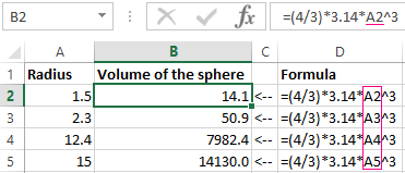
As you can see, the relative addresses help to change the address in each formula automatically.
It is also worth to point the regularity of changes in references of formulas. Data in B3 refers to A3, B4 to A4, and so on. Everything depends on where the first introduced formula will refer, and its copies will change the references relative to its position in the range of cells on the sheet.
Now instead of numbers we use absolute references:
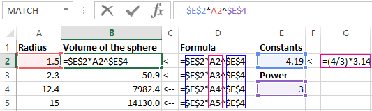
The result of the calculation is the same, but the formulas are more flexible to the changes. It is enough to change the value in one cell and the whole column is recalculated automatically. See the following example.
Use of absolute and relative links in Excel
Fill in the plate, as shown in the picture:
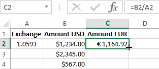
Description of the source table. In cell A2, there is an actual euro exchange rate against the dollar for today. In the range of cells B2: B4 are the amounts in dollars. In the range C2: C4 will be the amount in euros after the conversion of currencies. Tomorrow the course will change and the task of the plate will automatically recalculate the range of C2: C4 depending on the change in the value in cell A2 (that is, the euro rate).
To solve this problem, we need to enter a formula in C2: = B2 / A2 and copy it to all cells in the C2: C4 range. But here there is a problem. From the previous example, we know that when copying, relative references automatically change addresses relative to their position. Therefore, an error occurs:
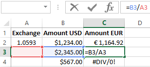
Concerning the first argument, this is quite acceptable. After all, the formula automatically refers to the new value in the column of the table cells (dollar amounts). But the second indicator we need to fix on the address A2. Accordingly, it is necessary to change the relative reference to the absolute in the formula.
How to make an absolute reference in Excel? It is very simple to put the $ (dollar) symbol before the line or column number or before the both of them. Below, consider all 3 options and determine their differences.
Our new formula should contain at once 2 types of links: absolute and relative.
- In C2, enter another formula: = B2 / A $ 2. To change links in Excel, double click on the cell with the left mouse button or press the F2 key on the keyboard.
- Copy it to the other cells in the C3:C4 range.
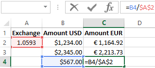
Description of the new formula. The dollar symbol ($) in the address of references fixes the address in the new copied formulas.
Absolute, relative and mixed references in Excel:
- $ A $ 2 — address of the absolute reference with fixation on columns and rows, both vertically and horizontally.
- $ A2 is a mixed link. When copying a column is fixed, and the row is changed.
- A $ 2 is a mixed link. When copying a row is fixed, and the column is changed.
For comparison: A2 is a relative address, without fixation. During the copying of the formulas, the row (2) and the column (A) automatically change to the new addresses relative to the location of the copied formula, both vertically and horizontally.
Note. In this example, the formula can contain not only a mixed link, but the absolute result: = B2 / $ A $ 2. The result will be the same. But in practice, there are often cases when you cannot do a thing without mixed references.
Helpful advice. To avoid entering the dollar symbol ($) manually, after specifying the address, press F4 repeatedly to select the required type: absolute or mixed. It’s fast and convenient.
Содержание
- HYPERLINK function
- Description
- Syntax
- Remark
- Examples
- Create an external reference (link) to a cell range in another workbook
- Create an external reference between cells in different workbooks
- Create a link to a worksheet in the same workbook
- Need more help?
- Create or change a cell reference
- Need more help?
HYPERLINK function
This article describes the formula syntax and usage of the HYPERLINK function in Microsoft Excel.
Description
The HYPERLINK function creates a shortcut that jumps to another location in the current workbook, or opens a document stored on a network server, an intranet, or the Internet. When you click a cell that contains a HYPERLINK function, Excel jumps to the location listed, or opens the document you specified.
Syntax
The HYPERLINK function syntax has the following arguments:
Link_location Required. The path and file name to the document to be opened. Link_location can refer to a place in a document — such as a specific cell or named range in an Excel worksheet or workbook, or to a bookmark in a Microsoft Word document. The path can be to a file that is stored on a hard disk drive. The path can also be a universal naming convention (UNC) path on a server (in Microsoft Excel for Windows) or a Uniform Resource Locator (URL) path on the Internet or an intranet.
Note Excel for the web the HYPERLINK function is valid for web addresses (URLs) only. Link_location can be a text string enclosed in quotation marks or a reference to a cell that contains the link as a text string.
If the jump specified in link_location does not exist or cannot be navigated, an error appears when you click the cell.
Friendly_name Optional. The jump text or numeric value that is displayed in the cell. Friendly_name is displayed in blue and is underlined. If friendly_name is omitted, the cell displays the link_location as the jump text.
Friendly_name can be a value, a text string, a name, or a cell that contains the jump text or value.
If friendly_name returns an error value (for example, #VALUE!), the cell displays the error instead of the jump text.
In the Excel desktop application, to select a cell that contains a hyperlink without jumping to the hyperlink destination, click the cell and hold the mouse button until the pointer becomes a cross  , then release the mouse button. In Excel for the web, select a cell by clicking it when the pointer is an arrow; jump to the hyperlink destination by clicking when the pointer is a pointing hand.
Examples
=HYPERLINK(«http://example.microsoft.com/report/budget report.xlsx», «Click for report»)
Opens a workbook saved at http://example.microsoft.com/report. The cell displays «Click for report» as its jump text.
=HYPERLINK(«[http://example.microsoft.com/report/budget report.xlsx]Annual!F10», D1)
Creates a hyperlink to cell F10 on the Annual worksheet in the workbook saved at http://example.microsoft.com/report. The cell on the worksheet that contains the hyperlink displays the contents of cell D1 as its jump text.
=HYPERLINK(«[http://example.microsoft.com/report/budget report.xlsx]’First Quarter’!DeptTotal», «Click to see First Quarter Department Total»)
Creates a hyperlink to the range named DeptTotal on the First Quarter worksheet in the workbook saved at http://example.microsoft.com/report. The cell on the worksheet that contains the hyperlink displays «Click to see First Quarter Department Total» as its jump text.
=HYPERLINK(«http://example.microsoft.com/Annual Report.docx]QrtlyProfits», «Quarterly Profit Report»)
To create a hyperlink to a specific location in a Word file, you use a bookmark to define the location you want to jump to in the file. This example creates a hyperlink to the bookmark QrtlyProfits in the file Annual Report.doc saved at http://example.microsoft.com.
Displays the contents of cell D5 as the jump text in the cell and opens the workbook saved on the FINANCE server in the Statements share. This example uses a UNC path.
Opens the workbook 1stqtr.xlsx that is stored in the Finance directory on drive D, and displays the numeric value that is stored in cell H10.
Creates a hyperlink to the Totals area in another (external) workbook, Mybook.xlsx.
=HYPERLINK(«[Book1.xlsx]Sheet1!A10″,»Go to Sheet1 > A10»)
To jump to a different location in the current worksheet, include both the workbook name, and worksheet name like this, where Sheet1 is the current worksheet.
=HYPERLINK(«[Book1.xlsx]January!A10″,»Go to January > A10»)
To jump to a different location in the current worksheet, include both the workbook name, and worksheet name like this, where January is another worksheet in the workbook.
=HYPERLINK(CELL(«address»,January!A1),»Go to January > A1″)
To jump to a different location in the current worksheet without using the fully qualified worksheet reference ([Book1.xlsx]), you can use this, where CELL(«address») returns the current workbook name.
To quickly update all formulas in a worksheet that use a HYPERLINK function with the same arguments, you can place the link target in another cell on the same or another worksheet, and then use an absolute reference to that cell as the link_location in the HYPERLINK formulas. Changes that you make to the link target are immediately reflected in the HYPERLINK formulas.
Источник
Create an external reference (link) to a cell range in another workbook
You can refer to the contents of cells in another workbook by creating an external reference formula. An external reference (also called a link) is a reference to a cell or range on a worksheet in another Excel workbook, or a reference to a defined name in another workbook.
Open the workbook that will contain the external reference (the destination workbook) and the workbook that contains the data that you want to link to (the source workbook).
Select the cell or cells where you want to create the external reference.
Type = (equal sign).
If you want to use a function, such as SUM, then type the function name followed by an opening parenthesis. For example, =SUM(.
Switch to the source workbook, and then click the worksheet that contains the cells that you want to link.
Select the cell or cells that you want to link to and press Enter.
Note: If you select multiple cells, like =[SourceWorkbook.xlsx]Sheet1!$A$1:$A$10, and have a current version of Microsoft 365, then you can simply press ENTER to confirm the formula as a dynamic array formula. Otherwise, the formula must be entered as a legacy array formula by pressing CTRL+SHIFT+ENTER. For more information on array formulas, see Guidelines and examples of array formulas.
Excel will return you to the destination workbook and display the values from the source workbook.
Note that Excel will return the link with absolute references, so if you want to copy the formula to other cells, you’ll need to remove the dollar ($) signs:
=[SourceWorkbook.xlsx]Sheet1! $A $1
If you close the source workbook, Excel will automatically append the file path to the formula:
Open the workbook that will contain the external reference (the destination workbook) and the workbook that contains the data that you want to link to (the source workbook).
Select the cell or cells where you want to create the external reference.
Type = (equal sign).
Switch to the source workbook, and then click the worksheet that contains the cells that you want to link.
Press F3, select the name that you want to link to and press Enter.
Note: If the named range references multiple cells, and you have a current version of Microsoft 365, then you can simply press ENTER to confirm the formula as a dynamic array formula. Otherwise, the formula must be entered as a legacy array formula by pressing CTRL+SHIFT+ENTER. For more information on array formulas, see Guidelines and examples of array formulas.
Excel will return you to the destination workbook and display the values from the named range in the source workbook.
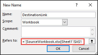
Open the destination workbook and the source workbook.
In the destination workbook, Go to Formulas > Defined Names > Define Name.
In the New Name dialog box, in the Name box, type a name for the range.
In the Refers to box, delete the contents, and then keep the cursor in the box.
If you want the name to use a function, enter the function name, and then position the cursor where you want the external reference. For example, type =SUM(), and then position the cursor between the parentheses.
Switch to the source workbook, and then click the worksheet that contains the cells that you want to link.
Select the cell or range of cells that you want to link, and click OK.
 Defined Names > Define Name > New Name.» loading=»lazy»>
External references are especially useful when it’s not practical to keep large worksheet models together in the same workbook.
Merge data from several workbooks You can link workbooks from several users or departments and then integrate the pertinent data into a summary workbook. That way, when the source workbooks are changed, you won’t have to manually change the summary workbook.
Create different views of your data You can enter all of your data into one or more source workbooks, and then create a report workbook that contains external references to only the pertinent data.
Streamline large, complex models By breaking down a complicated model into a series of interdependent workbooks, you can work on the model without opening all of its related sheets. Smaller workbooks are easier to change, don’t require as much memory, and are faster to open, save, and calculate.
Formulas with external references to other workbooks are displayed in two ways, depending on whether the source workbook — the one that supplies data to a formula — is open or closed.
When the source is open, the external reference includes the workbook name in square brackets ( [ ]), followed by the worksheet name, an exclamation point ( !), and the cells that the formula depends on. For example, the following formula adds the cells C10:C25 from the workbook named Budget.xls.
When the source is not open, the external reference includes the entire path.
Note: If the name of the other worksheet or workbook contains spaces or non-alphabetical characters, you must enclose the name (or the path) within single quotation marks as in the example above. Excel will automatically add these for you when you select the source range.
Formulas that link to a defined name in another workbook use the workbook name followed by an exclamation point (!) and the name. For example, the following formula adds the cells in the range named Sales from the workbook named Budget.xlsx.
Select the cell or cells where you want to create the external reference.
Type = (equal sign).
If you want to use a function, such as SUM, then type the function name followed by an opening parenthesis. For example, =SUM(.
Switch to the worksheet that contains the cells that you want to link to.
Select the cell or cells that you want to link to and press Enter.
Note: If you select multiple cells (=Sheet1!A1:A10), and have a current version of Microsoft 365, then you can simply press ENTER to confirm the formula as a dynamic array formula. Otherwise, the formula must be entered as a legacy array formula by pressing CTRL+SHIFT+ENTER. For more information on array formulas, see Guidelines and examples of array formulas.
Excel will return to the original worksheet and display the values from the source worksheet.
Create an external reference between cells in different workbooks
Open the workbook that will contain the external reference (the destination workbook, also called the formula workbook) and the workbook that contains the data that you want to link to (the source workbook, also called the data workbook).
In the source workbook, select the cell or cells you want to link.
Press Ctrl+C or go to Home > Clipboard > Copy.
Switch to the destination workbook, and then click the worksheet where you want the linked data to be placed.
Select the cell where you want to place the linked data, then go to Home > Clipboard > Paste > Paste Link.
Excel will return the data you copied from the source workbook. If you change it, it will automatically change in the destination workbook when you refresh your browser window.
To use the link in a formula, type = in front of the link, choose a function, type (, and then type ) after the link.
Create a link to a worksheet in the same workbook
Select the cell or cells where you want to create the external reference.
Type = (equal sign).
If you want to use a function, such as SUM, then type the function name followed by an opening parenthesis. For example, =SUM(.
Switch to the worksheet that contains the cells that you want to link to.
Select the cell or cells that you want to link to and press Enter.
Excel will return to the original worksheet and display the values from the source worksheet.
Need more help?
You can always ask an expert in the Excel Tech Community or get support in the Answers community.
Источник
Create or change a cell reference
A cell reference refers to a cell or a range of cells on a worksheet and can be used in a formula so that Microsoft Office Excel can find the values or data that you want that formula to calculate.
In one or several formulas, you can use a cell reference to refer to:
Data from one or more contiguous cells on the worksheet.
Data contained in different areas of a worksheet.
Data on other worksheets in the same workbook.
The value in cell C2.
Cells A1 through F4
The values in all cells, but you must press Ctrl+Shift+Enter after you type in your formula.
Note: This functionality doesn’t work in Excel for the web.
The cells named Asset and Liability
The value in the cell named Liability subtracted from the value in the cell named Asset.
The cell ranges named Week1 and Week2
The sum of the values of the cell ranges named Week1 and Week 2 as an array formula.
Cell B2 on Sheet2
The value in cell B2 on Sheet2.
Click the cell in which you want to enter the formula.
In the formula bar  , type = (equal sign).
Do one of the following:
Reference one or more cells To create a reference, select a cell or range of cells on the same worksheet.
You can drag the border of the cell selection to move the selection, or drag the corner of the border to expand the selection.
Reference a defined name To create a reference to a defined name, do one of the following:
Press F3, select the name in the Paste name box, and then click OK.
Note: If there is no square corner on a color-coded border, the reference is to a named range.
Do one of the following:
If you are creating a reference in a single cell, press Enter.
If you are creating a reference in an array formula (such A1:G4), press Ctrl+Shift+Enter.
The reference can be a single cell or a range of cells, and the array formula can be one that calculates single or multiple results.
Note: If you have a current version of Microsoft 365, then you can simply enter the formula in the top-left-cell of the output range, then press ENTER to confirm the formula as a dynamic array formula. Otherwise, the formula must be entered as a legacy array formula by first selecting the output range, entering the formula in the top-left-cell of the output range, and then pressing CTRL+SHIFT+ENTER to confirm it. Excel inserts curly brackets at the beginning and end of the formula for you. For more information on array formulas, see Guidelines and examples of array formulas.
You can refer to cells that are on other worksheets in the same workbook by prepending the name of the worksheet followed by an exclamation point ( !) to the start of the cell reference. In the following example, the worksheet function named AVERAGE calculates the average value for the range B1:B10 on the worksheet named Marketing in the same workbook.

1. Refers to the worksheet named Marketing
2. Refers to the range of cells between B1 and B10, inclusively
3. Separates the worksheet reference from the cell range reference
Click the cell in which you want to enter the formula.
In the formula bar , type = (equal sign) and the formula you want to use.
Click the tab for the worksheet to be referenced.
Select the cell or range of cells to be referenced.
Note: If the name of the other worksheet contains nonalphabetical characters, you must enclose the name (or the path) within single quotation marks ( ‘).
Alternatively, you can copy and paste a cell reference and then use the Link Cells command to create a cell reference. You can use this command to:
Easily display important information in a more prominent position. Let’s say that you have a workbook that contains many worksheets, and on each worksheet is a cell that displays summary information about the other cells on that worksheet. To make these summary cells more prominent, you can create a cell reference to them on the first worksheet of the workbook, which enables you to see summary information about the whole workbook on the first worksheet.
Make it easier to create cell references between worksheets and workbooks. The Link Cells command automatically pastes the correct syntax for you.
Click the cell that contains the data you want to link to.
Press Ctrl+C, or go to the Home tab, and in the Clipboard group, click Copy  .
.

Press Ctrl+V, or go to the Home tab, in the Clipboard group, click Paste  .
.
By default, the Paste Options  button appears when you paste copied data.
Click the Paste Options button, and then click Paste Link  .
.
Double-click the cell that contains the formula that you want to change. Excel highlights each cell or range of cells referenced by the formula with a different color.
Do one of the following:
To move a cell or range reference to a different cell or range, drag the color-coded border of the cell or range to the new cell or range.
To include more or fewer cells in a reference, drag a corner of the border.
In the formula bar , select the reference in the formula, and then type a new reference.
Press F3, select the name in the Paste name box, and then click OK.
Press Enter, or, for an array formula, press Ctrl+Shift+Enter.
Note: If you have a current version of Microsoft 365, then you can simply enter the formula in the top-left-cell of the output range, then press ENTER to confirm the formula as a dynamic array formula. Otherwise, the formula must be entered as a legacy array formula by first selecting the output range, entering the formula in the top-left-cell of the output range, and then pressing CTRL+SHIFT+ENTER to confirm it. Excel inserts curly brackets at the beginning and end of the formula for you. For more information on array formulas, see Guidelines and examples of array formulas.
Frequently, if you define a name to a cell reference after you enter a cell reference in a formula, you may want to update the existing cell references to the defined names.
Do one of the following:
Select the range of cells that contains formulas in which you want to replace cell references with defined names.
Select a single, empty cell to change the references to names in all formulas on the worksheet.
On the Formulas tab, in the Defined Names group, click the arrow next to Define Name, and then click Apply Names.
In the Apply names box, click one or more names, and then click OK.
Select the cell that contains the formula.
In the formula bar , select the reference that you want to change.
Press F4 to switch between the reference types.
For more information about the different type of cell references, see Overview of formulas.
Click the cell in which you want to enter the formula.
In the formula bar , type = (equal sign).
Select a cell or range of cells on the same worksheet. You can drag the border of the cell selection to move the selection, or drag the corner of the border to expand the selection.
Do one of the following:
If you are creating a reference in a single cell, press Enter.
If you are creating a reference in an array formula (such A1:G4), press Ctrl+Shift+Enter.
The reference can be a single cell or a range of cells, and the array formula can be one that calculates single or multiple results.
Note: If you have a current version of Microsoft 365, then you can simply enter the formula in the top-left-cell of the output range, then press ENTER to confirm the formula as a dynamic array formula. Otherwise, the formula must be entered as a legacy array formula by first selecting the output range, entering the formula in the top-left-cell of the output range, and then pressing CTRL+SHIFT+ENTER to confirm it. Excel inserts curly brackets at the beginning and end of the formula for you. For more information on array formulas, see Guidelines and examples of array formulas.
You can refer to cells that are on other worksheets in the same workbook by prepending the name of the worksheet followed by an exclamation point ( !) to the start of the cell reference. In the following example, the worksheet function named AVERAGE calculates the average value for the range B1:B10 on the worksheet named Marketing in the same workbook.
1. Refers to the worksheet named Marketing
2. Refers to the range of cells between B1 and B10, inclusively
3. Separates the worksheet reference from the cell range reference
Click the cell in which you want to enter the formula.
In the formula bar , type = (equal sign) and the formula you want to use.
Click the tab for the worksheet to be referenced.
Select the cell or range of cells to be referenced.
Note: If the name of the other worksheet contains nonalphabetical characters, you must enclose the name (or the path) within single quotation marks ( ‘).
Double-click the cell that contains the formula that you want to change. Excel highlights each cell or range of cells referenced by the formula with a different color.
Do one of the following:
To move a cell or range reference to a different cell or range, drag the color-coded border of the cell or range to the new cell or range.
To include more or fewer cells in a reference, drag a corner of the border.
In the formula bar , select the reference in the formula, and then type a new reference.
Press Enter, or, for an array formula, press Ctrl+Shift+Enter.
Note: If you have a current version of Microsoft 365, then you can simply enter the formula in the top-left-cell of the output range, then press ENTER to confirm the formula as a dynamic array formula. Otherwise, the formula must be entered as a legacy array formula by first selecting the output range, entering the formula in the top-left-cell of the output range, and then pressing CTRL+SHIFT+ENTER to confirm it. Excel inserts curly brackets at the beginning and end of the formula for you. For more information on array formulas, see Guidelines and examples of array formulas.
Select the cell that contains the formula.
In the formula bar , select the reference that you want to change.
Press F4 to switch between the reference types.
For more information about the different type of cell references, see Overview of formulas.
Need more help?
You can always ask an expert in the Excel Tech Community or get support in the Answers community.
Источник
In Excel, copying data from one worksheet to another is an easy task, but there is not any link between the two. But we can create a link between two worksheets or workbooks to automatically update data in another sheet if it changes in the first worksheet. This article explains how this is done.
Automatically data in another sheet in Excel
We can link worksheets and update data automatically. A link is a dynamic formula that pulls data from a cell of one worksheet and automatically updates that data to another worksheet. These linking worksheets can be in the same workbook or in another workbook.
One worksheet is called the source worksheet, from where this link pulls the data automatically, and the other worksheet is called the destination worksheet that contains that link formula and where data is updated automatically.
Remember one thing that formatting of cells of source worksheet and destination worksheet should be the same otherwise the result could be viewed differently and can lead to confusion.
Two methods of linking data in different worksheets
We can link these two worksheets using two different methods.
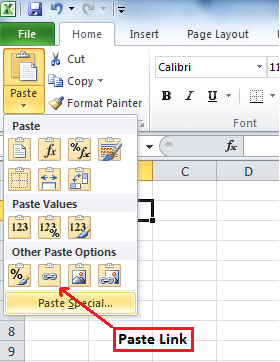
- Copy and Paste Link
- From source worksheet, select the cell that contains data or that you want to link to another worksheet, and copy it by pressing the Copy button from the Home tab or press CTRL+C.
- Go to the destination worksheet and click the cell where you want to link the cell from the source worksheet. On the Home tab, click on the drop-down arrow button of Paste, and select Paste Link from “Other Paste Options.” Or right-click in the cell on the destination worksheet and choose Paste Link from Paste Options.
- Save the work or return to the source workbook and press ESC button on the keyboard to remove the border around the copied cell and save the work.
- Enter formula manually
- In the destination worksheet, click on the cell that will contain link formula and enter an equal sign (=)
- Go to the source sheet and click on the cell that contains data and press Enter on the keyboard. Save your work.
Using these two methods, we can link a worksheet and update data automatically depending upon your requirements. In this article, we will discuss some examples using the following cases.
Update cell on one worksheet based on a cell on another sheet
Suppose we have a value of 200 in cell A1 on Sheet1 and want to update cell A1 on Sheet2 using the linking formula. We can do that by using the same two methods we’ve covered.
Using Copy and Paste Link method
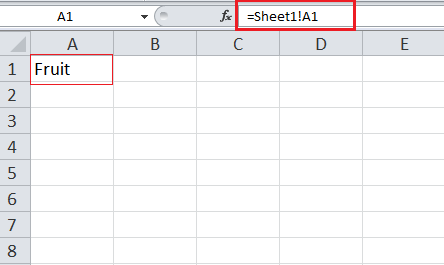
Copy the cell value of 200 from cell A1 on Sheet1.

Go to Sheet2, click in cell A1 and click on the drop-down arrow of Paste button on the Home tab and select Paste Link button. It will generate a link by automatically entering the formula =Sheet1!A1.

Or right-click in the cell on the destination worksheet, Sheet2, and choose Paste Link from Paste Options: It will generate linking formula automatically.

Entering formula manually
We can enter the linking formula manually in cell A1 on the destination worksheet Sheet2 to update data by pulling it from cell A1 of Sheet1.
In cell A1 on Sheet2, manually enter an equal sign (=) and go to Sheet1 and click on cell A1 and press ENTER key on your keyboard. The following linking formula will be updated in destination sheet that will link cell A1 of both sheets.
=Sheet1!A1
Update cell on one sheet only if the first sheet meets a condition
By entering the linking formula manually, we can update data in cell A1 of Sheet2 based on a condition if the cell value of A1 on Sheet1 is greater than 200. We can do that by entering this logical condition in an IF function. If cell A1 on Sheet1 meets this condition then IF function returns the value in cell A1 on Sheet2 otherwise it will return blank cell.
Here is the formula to link the cells of both sheets based on this condition. We will enter this formula manually in cell A1 of Sheet2
=IF(Sheet1!A1>200,Sheet1!A1,"")

Update cell on one sheet from another sheet with a drop-down list
Suppose we have a drop-down list in cell A1 of Sheet1 and we can update cell A1 on Sheet2 by entering link formula in cell A1 on Sheet2.

In cell A1 on Sheet2, we will manually enter this linking formula to update data automatically based on the cell value selected from the drop-down list.
=Sheet1!A1
Linking data in a real data set is more complex and depends on your situation. You might need to use techniques other than those listed above. If you are in a rush and want your problem answered by an Excel expert, try our service. The experts are available to help you 24/7. The first question is free.
As you use and build more Excel workbooks, you’ll need to link them up. Maybe you want to write formulas that use data between different sheets in a workbook. You can even write formulas that use data from multiple different workbooks.
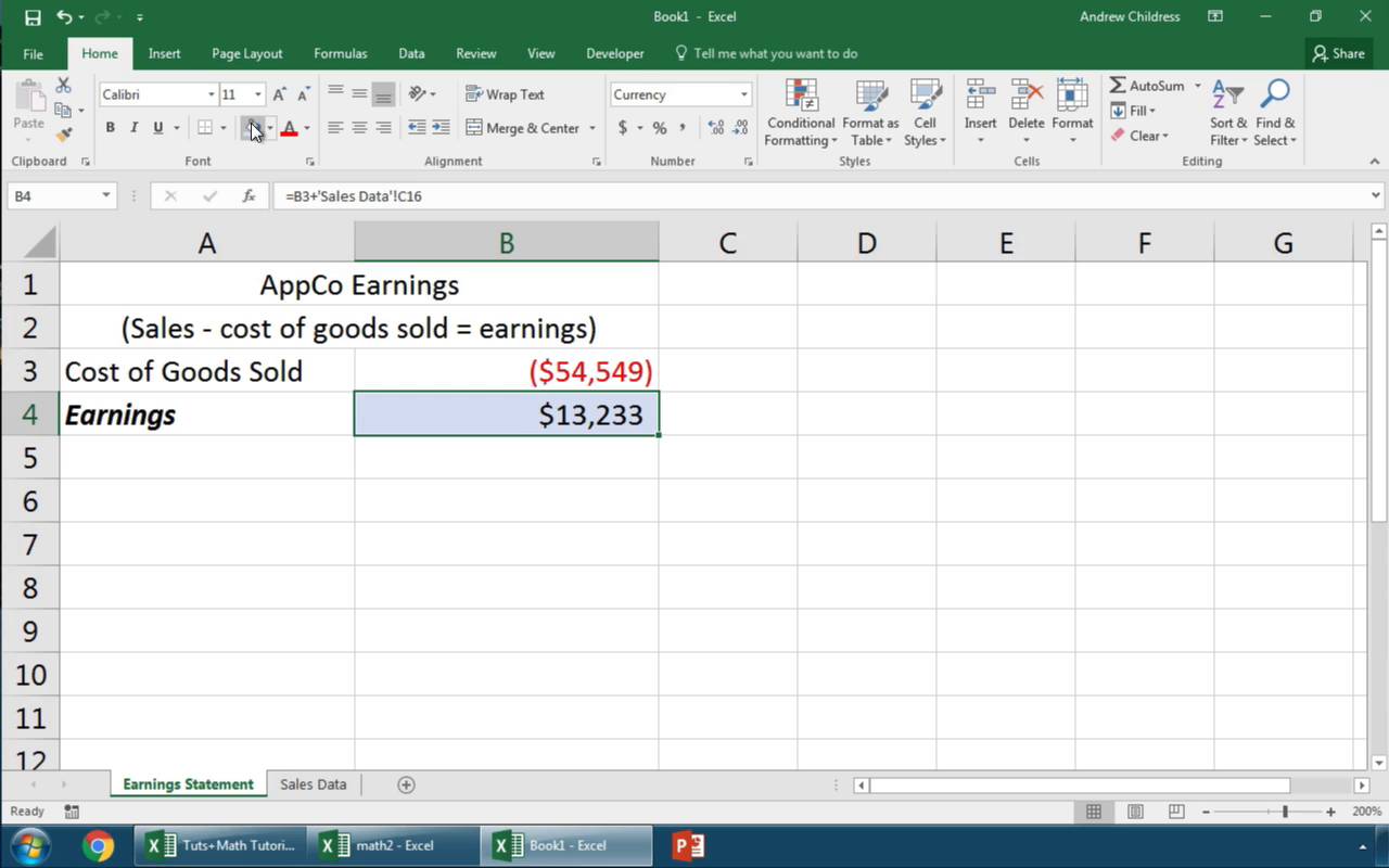
If I want to keep my files clean and tidy, I’ve found it’s best to separate large sheets of data from the formulas that summarize them. I often use a single workbook or sheet to summarize things.
In this tutorial, you’ll learn how to link data in Excel. First, we’ll learn how to link up data in the same workbook on different sheets. Then, we’ll move on to linking up multiple Excel workbooks to import and sync data between files.
How to Quickly Link Data in Excel Workbooks (Watch & Learn)
I’ll walk you through two examples linking up your spreadsheets. You’ll see how to pull data from another workbook in Excel and keep two workbooks connected. We’ll also walk through a basic example to write formulas between sheets in the same workbook.
Let’s walk through an illustrated guide to linking up your data between sheets and workbooks in Excel.
Basics: How to Link Between Sheets in Excel
Let’s start off by learning how to write formulas using data from another sheet. You probably already know that Excel workbooks can contain multiple worksheets. Each worksheet is a tab of its own, and you can switch tabs by clicking on them at the bottom of Excel.
Complex workbooks can easily grow to many sheets. In time, you’ll certainly need to write formulas to work with data on different tabs.
Maybe you use a single sheet in your workbook for all of your formulas to summarize your data, and separate sheets to hold the original data.

Let’s learn how to write a multi-sheet formula to work with data from multiple sheets in the same workbook.
1. Start a New Formula in Excel
Most formulas in Excel start off with the equals (=) sign. Double click or start typing in a cell and begin writing the formula that you want to link up. For my example, I’ll write a sum formula to add up several cells.
I’ll open up the = sign, and then click on the first cell on my current sheet to make it the first part of the formula. Then, I’ll type a + sign to add my second cell to this formula.
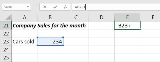

Now, make sure that you don’t close out your formula and press enter yet! You’ll want to leave the formula open before you switch sheets.
2. Switch Sheets in Excel
While you still have the formula open, click on a different sheet tab at the bottom of Excel. It’s very important that you don’t close out the formula before you click on the next cell to include as part of the formula.
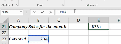

After you switch sheets, click on the next cell that you want to include in the formula. As you can see in the screenshot below, Excel automatically writes the part of the formula that references a cell on another sheet for you.
Notice in the screenshot below that to reference a cell on another sheet, Excel adds «Sheet2!B3», which simply references cell B3 on a sheet named Sheet2. You could write this manually, but clicking on the cells makes Excel write it for you automatically.
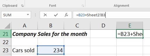

3. Finish the Excel Formula
At this point, you can press enter to close out and complete your multi-sheet formula. When you do so, Excel will jump back to where you started the formula and show you the results.
You could also keep writing the formula, including cells from more sheets and other cells on the same sheet. Keep combining those references throughout the workbook for all the data you need.
Level Up: How to Link Multiple Excel Workbooks
Let’s learn how to pull data from another workbook. With this skill, you can write formulas that pull together data from entirely separate Excel workbooks.
For this section of the tutorial, you can use two workbooks that you can download for free as a part of this tutorial. Open them both up in Excel, and follow the directions below.
1. Open Both Workbooks
Let’s start off by writing a formula that includes data from two different workbooks.
The easiest way to use this feature is to open up two Excel workbooks at the same time and put them side by side. I use the Windows Snap feature to split them to each take up half the screen. You need to keep both workbooks in view to write formulas between them.
In the screenshot below, I’ve opened two workbooks that I’ll write formulas for side-by-side. For my example, I’m running a business that buys a variety of products, and sells them in a variety of countries. So, I’ll use separate workbooks to track my purchases/sales and cost data.
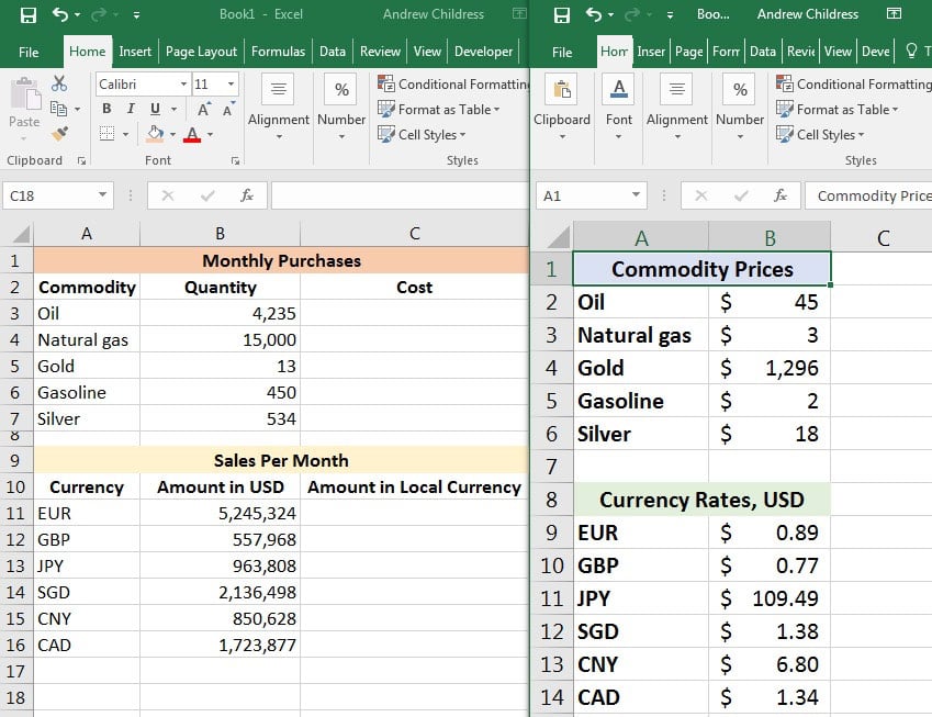

2. Start Writing Your Formula in Excel
The price of what I buy can change, and so can the rate that I receive payments in. I need to keep a lookup list of rates and multiply it times my purchases. This is the perfect time to link two workbooks together and write formulas between them.
Let’s take the number of barrels of oil I buy each month times the price per barrel. In the first Cost cell (cell C3), I’ll start writing a formula by typing the equals sign (=), and then clicking on cell B3 to grab the quantity. Now, I’ll add an * to prepare to multiply the quantity by the rate.
So far, your formula should be:
=B3*


Don’t close out your formula yet. Make sure to leave it open before moving onto the next step; we still need to point Excel to the price data to multiply the quantity by.
3. Switch Excel Workbooks
It’s time to switch workbooks, and this is why it’s important to keep both of your datasets in view while working between workbooks.
With your formula still open, click over to the other workbook. Then, click on a cell in your second workbook to link up the two Excel files.


Excel automatically wrote the reference to a separate workbook as part of the cell formula:
=B3*[Prices.xlsx]Sheet1!$B$2
Once you press Enter, Excel will calculate the final cost by multiplying the quantity in the first workbook times the price in the second workbook.
Now, keep working on your Excel skills by multiplying each of the quantities or values times the reference amounts in the «Prices» workbook.
In short, the key is to get your workbooks open side by side, and simply switch workbooks to write formulas referencing other files.
There’s nothing stopping you from linking up more than two workbooks. You could open many workbooks to link up and write formulas, connecting the data between many sheets to keep cells up to date.
How to Refresh Your Data Between Workbooks
When you’ve written formulas that reference other Excel workbooks, you’ll need to think about how you’ll update your data.
So, what happens when the data changes in the workbook that you’re linking to? Will your workbook automatically update, or will you need to refresh your files to pull over the last data and import it?
The answer is, «it depends», and specifically, it depends upon if both workbooks are still open at the same time.
Example 1: Both Excel Workbooks Still Open
Let’s check out an example using the same workbook from the prior step. Both workbooks are still open. Let’s see what happens when we change the price of oil from $45 per barrel to $75 per barrel:


In the screenshot above, you can see that when we updated the price of oil, the other workbook automatically updated.
This is important to know: if both workbooks are open at the same time, changes will update automatically and in real-time. When you change one variable, the other workbook will update or recalculate based upon the new value.
Example 2: With One Workbook Closed
What if you only open one workbook at a time? For example, each morning, we update prices of our commodities and currencies, and in the evening we review the impact of the change to our purchases and sales.
The next time you open up your workbook that references other sheets, you might get a message similar to the one below. You can click on Update to pull in the latest data from your reference workbook.
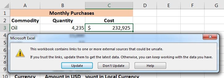


You might also see a menu where you can click Enable Content to automate updating data between Excel files.
Recap and Keep Learning More About Excel
Writing formulas between sheets and workbooks is a necessary skill when you work with Microsoft Excel. Using multiple spreadsheets inside your formulas is no problem with a bit of know-how.
Check out these additional tutorials to learn more about Excel skills and how to work with data. These tutorials are a great way to continue learning Excel.
Let me know in the comments if you have any questions about how to link up your Excel workbooks.
Did you find this post useful?

I believe that life is too short to do just one thing. In college, I studied Accounting and Finance but continue to scratch my creative itch with my work for Envato Tuts+ and other clients. By day, I enjoy my career in corporate finance, using data and analysis to make decisions.
I cover a variety of topics for Tuts+, including photo editing software like Adobe Lightroom, PowerPoint, Keynote, and more. What I enjoy most is teaching people to use software to solve everyday problems, excel in their career, and complete work efficiently. Feel free to reach out to me on my website.