
Excel for Microsoft 365 Excel for Microsoft 365 for Mac Excel for the web More…Less
Linked data types connect to reputable sources of data, such as Bing, Power BI and more, so you can access information about a variety of subjects without ever leaving Excel. This page will be updated with what’s currently available.
Note: Linked data types are only available to Worldwide Multi-Tenant clients (Microsoft 365 accounts,) but data types from different sources may have different requirements. To check the source, select the data type icon in the cell of a converted data type > in the card, scroll to the bottom for the source name. For detailed requirements, see How to access data types in the FAQ.
List of linked data types in Excel
To open the data types gallery, go to the Data tab in Excel > Data Types group > expand the dropdown.
Note: Most data types require a Microsoft 365 subscription to use, but data types from different sources may have different requirements to use them. To check the requirements, see How to access data types in the FAQ. To check the source, select the data type icon in the cell of a converted data type to open the card, then scroll to the bottom for the source name.
|
Ribbon Button |
Includes these data types
|
|
|
|
|
|
exchange rates Powered by Bing USD/EUR, INR:AUD Tip: Make sure to insert two currencies separated by a «/» or a «:». |
|
|
country/region, city, state, administrative division, county, township, municipality, district, shire, province, territory, zip code Powered by Bing Seattle, United States |
|
|
Employee ID, Customer name |
More about linked data types
Linked data types FAQ and tips
Convert linked data types with Excel
How to write formulas that reference data types
Give feedback about data types
Need more help?
Want more options?
Explore subscription benefits, browse training courses, learn how to secure your device, and more.
Communities help you ask and answer questions, give feedback, and hear from experts with rich knowledge.
Excel for Microsoft 365 Excel for Microsoft 365 for Mac Excel for the web More…Less

Data on hundreds of subjects like cities, foods, animals, constellations, and more, all right in Excel. With linked data types, you gain access to a trusted database brimming with facts and data, templates to get things done, and more. These data types make it possible to accomplish goals for real life with the power and flexibility of Excel.
Data types transform the way you work with data
Real data for real life
Explore the universe or start a film club? With tons of data types with facts on a variety of subjects, the possibilities are almost limitless.
Convenience and efficiency
No more pasting from browsers or skimming search results. Data types make it easy to compile and bring facts from trusted sources right into Excel.
Use dynamic and flexible datasets
Easily explore data in Excel with interactive cards that hold a variety of data in a single cell. Insert, refresh, and work with data the way you want.
Start quickly with smart templates
Our data type templates help get things done fast, such as comparing colleges, tracking investments, planning a movie nights, and more.
Want more?
Linked data types FAQ and tips
Convert text to a linked data type in Excel
Stocks and geography data types
Discover more from Wolfram
Give feedback about data types
Need more help?
Содержание
- Создание связанных таблиц
- Способ 1: прямое связывание таблиц формулой
- Способ 2: использование связки операторов ИНДЕКС — ПОИСКПОЗ
- Способ 3: выполнение математических операций со связанными данными
- Способ 4: специальная вставка
- Способ 5: связь между таблицами в нескольких книгах
- Разрыв связи между таблицами
- Способ 1: разрыв связи между книгами
- Способ 2: вставка значений
- Вопросы и ответы

При выполнении определенных задач в Excel иногда приходится иметь дело с несколькими таблицами, которые к тому же связаны между собой. То есть, данные из одной таблицы подтягиваются в другие и при их изменении пересчитываются значения во всех связанных табличных диапазонах.
Связанные таблицы очень удобно использовать для обработки большого объема информации. Располагать всю информацию в одной таблице, к тому же, если она не однородная, не очень удобно. С подобными объектами трудно работать и производить по ним поиск. Указанную проблему как раз призваны устранить связанные таблицы, информация между которыми распределена, но в то же время является взаимосвязанной. Связанные табличные диапазоны могут находиться не только в пределах одного листа или одной книги, но и располагаться в отдельных книгах (файлах). Последние два варианта на практике используют чаще всего, так как целью указанной технологии является как раз уйти от скопления данных, а нагромождение их на одной странице принципиально проблему не решает. Давайте узнаем, как создавать и как работать с таким видом управления данными.
Создание связанных таблиц
Прежде всего, давайте остановимся на вопросе, какими способами существует возможность создать связь между различными табличными диапазонами.
Способ 1: прямое связывание таблиц формулой
Самый простой способ связывания данных – это использование формул, в которых имеются ссылки на другие табличные диапазоны. Он называется прямым связыванием. Этот способ интуитивно понятен, так как при нем связывание выполняется практически точно так же, как создание ссылок на данные в одном табличном массиве.
Посмотрим, как на примере можно образовать связь путем прямого связывания. Имеем две таблицы на двух листах. На одной таблице производится расчет заработной платы с помощью формулы путем умножения ставки работников на единый для всех коэффициент.
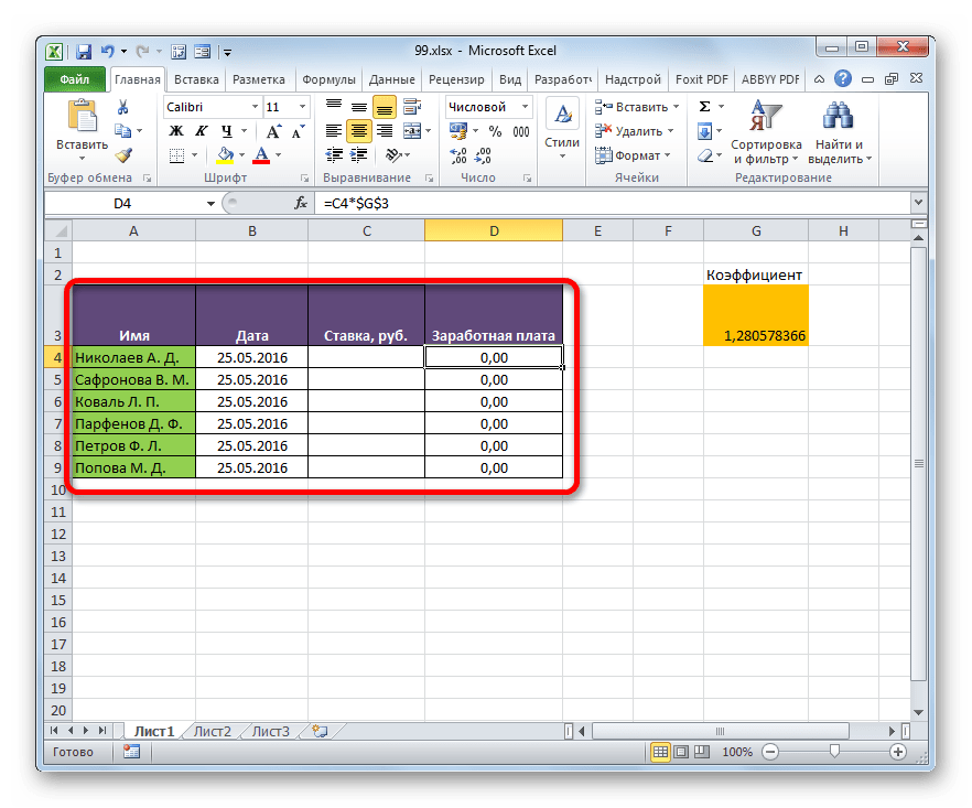
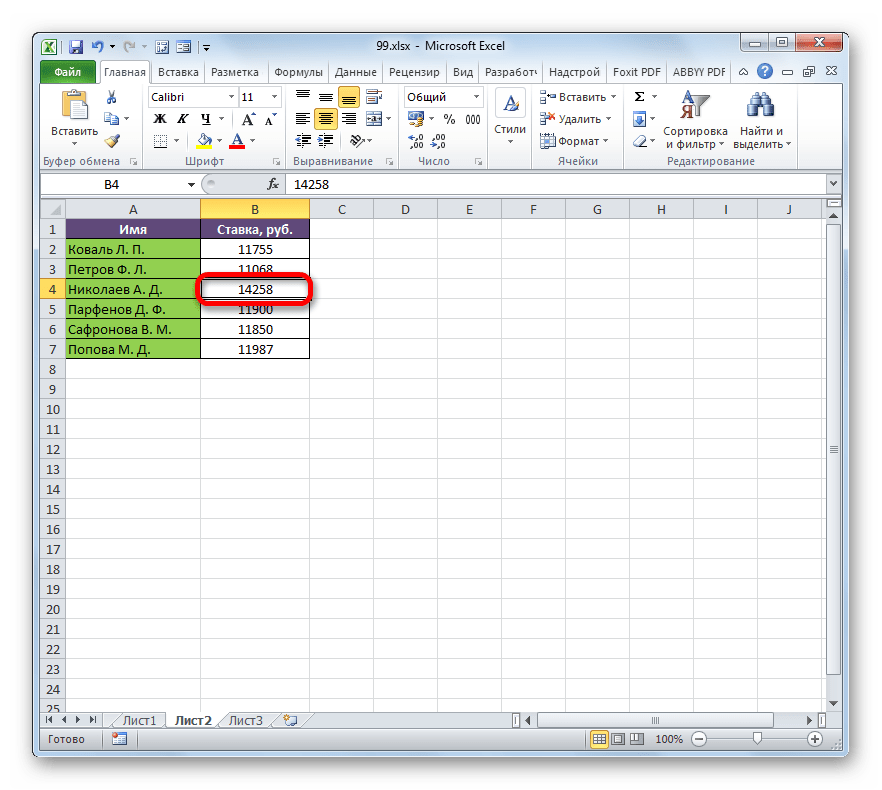
На втором листе расположен табличный диапазон, в котором находится перечень сотрудников с их окладами. Список сотрудников в обоих случаях представлен в одном порядке.
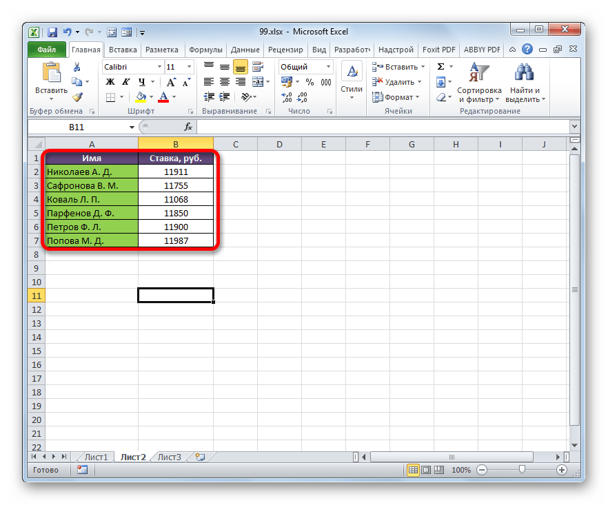
Нужно сделать так, чтобы данные о ставках из второго листа подтягивались в соответствующие ячейки первого.
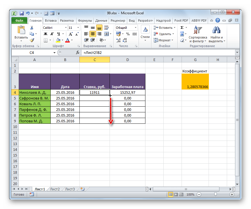
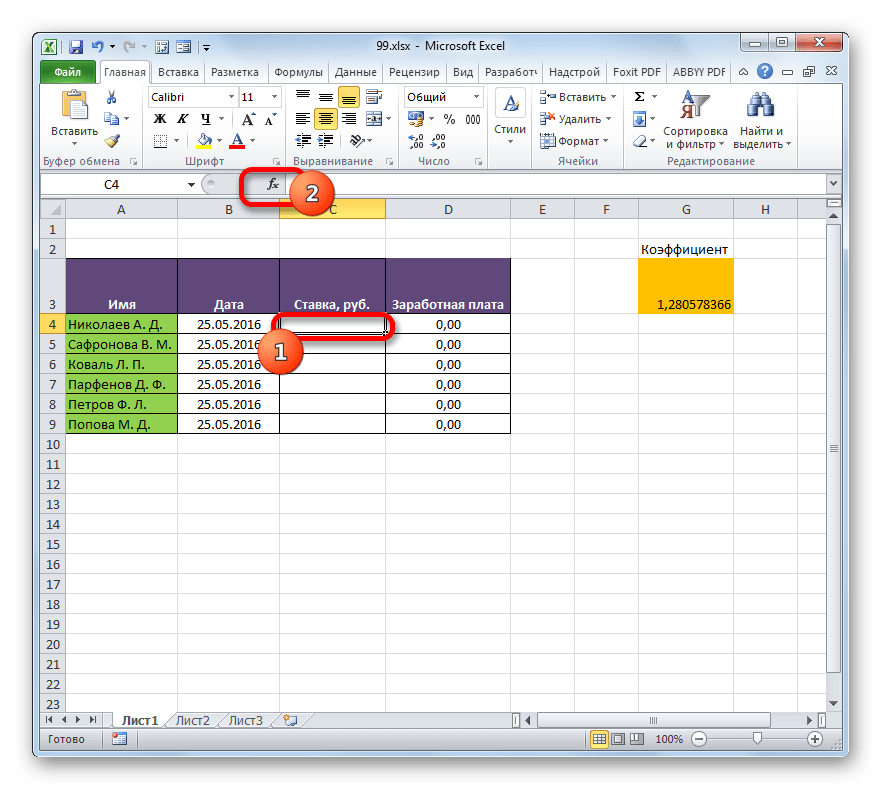
- На первом листе выделяем первую ячейку столбца «Ставка». Ставим в ней знак «=». Далее кликаем по ярлычку «Лист 2», который размещается в левой части интерфейса Excel над строкой состояния.
- Происходит перемещения во вторую область документа. Щелкаем по первой ячейке в столбце «Ставка». Затем кликаем по кнопке Enter на клавиатуре, чтобы произвести ввод данных в ячейку, в которой ранее установили знак «равно».
- Затем происходит автоматический переход на первый лист. Как видим, в соответствующую ячейку подтягивается величина ставки первого сотрудника из второй таблицы. Установив курсор на ячейку, содержащую ставку, видим, что для вывода данных на экран применяется обычная формула. Но перед координатами ячейки, откуда выводятся данные, стоит выражение «Лист2!», которое указывает наименование области документа, где они расположены. Общая формула в нашем случае выглядит так:
=Лист2!B2 - Теперь нужно перенести данные о ставках всех остальных работников предприятия. Конечно, это можно сделать тем же путем, которым мы выполнили поставленную задачу для первого работника, но учитывая, что оба списка сотрудников расположены в одинаковом порядке, задачу можно существенно упростить и ускорить её решение. Это можно сделать, просто скопировав формулу на диапазон ниже. Благодаря тому, что ссылки в Excel по умолчанию являются относительными, при их копировании происходит сдвиг значений, что нам и нужно. Саму процедуру копирования можно произвести с помощью маркера заполнения.
Итак, ставим курсор в нижнюю правую область элемента с формулой. После этого курсор должен преобразоваться в маркер заполнения в виде черного крестика. Выполняем зажим левой кнопки мыши и тянем курсор до самого низа столбца.
- Все данные из аналогичного столбца на Листе 2 были подтянуты в таблицу на Листе 1. При изменении данных на Листе 2 они автоматически будут изменяться и на первом.


Способ 2: использование связки операторов ИНДЕКС — ПОИСКПОЗ
Но что делать, если перечень сотрудников в табличных массивах расположен не в одинаковом порядке? В этом случае, как говорилось ранее, одним из вариантов является установка связи между каждой из тех ячеек, которые следует связать, вручную. Но это подойдет разве что для небольших таблиц. Для массивных диапазонов подобный вариант в лучшем случае отнимет очень много времени на реализацию, а в худшем – на практике вообще будет неосуществим. Но решить данную проблему можно при помощи связки операторов ИНДЕКС – ПОИСКПОЗ. Посмотрим, как это можно осуществить, связав данные в табличных диапазонах, о которых шел разговор в предыдущем способе.
- Выделяем первый элемент столбца «Ставка». Переходим в Мастер функций, кликнув по пиктограмме «Вставить функцию».
- В Мастере функций в группе «Ссылки и массивы» находим и выделяем наименование «ИНДЕКС».
- Данный оператор имеет две формы: форму для работы с массивами и ссылочную. В нашем случае требуется первый вариант, поэтому в следующем окошке выбора формы, которое откроется, выбираем именно его и жмем на кнопку «OK».
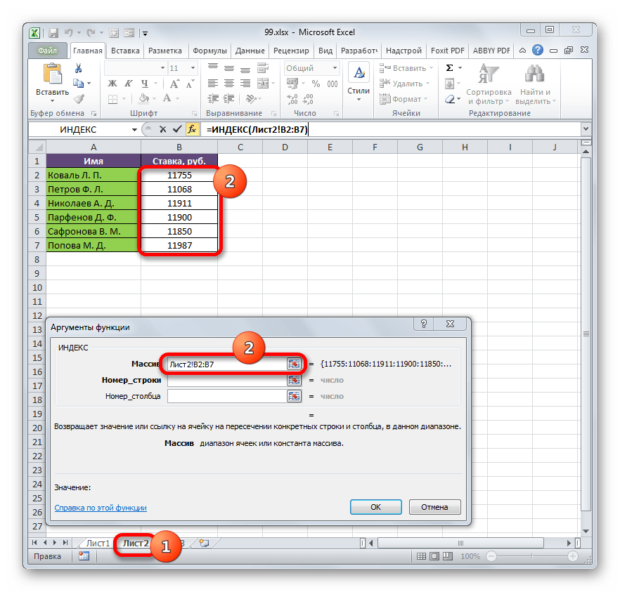
- Выполнен запуск окошка аргументов оператора ИНДЕКС. Задача указанной функции — вывод значения, находящегося в выбранном диапазоне в строке с указанным номером. Общая формула оператора ИНДЕКС такова:
=ИНДЕКС(массив;номер_строки;[номер_столбца])«Массив» — аргумент, содержащий адрес диапазона, из которого мы будем извлекать информацию по номеру указанной строки.
«Номер строки» — аргумент, являющийся номером этой самой строчки. При этом важно знать, что номер строки следует указывать не относительно всего документа, а только относительно выделенного массива.
«Номер столбца» — аргумент, носящий необязательный характер. Для решения конкретно нашей задачи мы его использовать не будем, а поэтому описывать его суть отдельно не нужно.
Ставим курсор в поле «Массив». После этого переходим на Лист 2 и, зажав левую кнопку мыши, выделяем все содержимое столбца «Ставка».
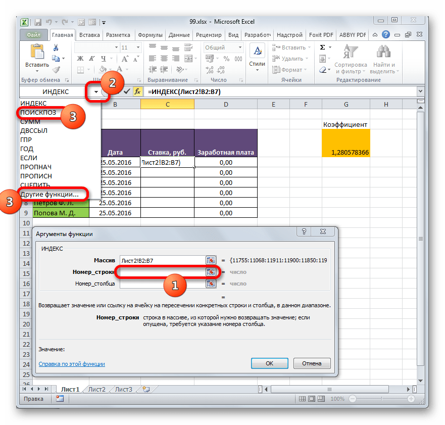
- После того, как координаты отобразились в окошке оператора, ставим курсор в поле «Номер строки». Данный аргумент мы будем выводить с помощью оператора ПОИСКПОЗ. Поэтому кликаем по треугольнику, который расположен слева от строки функций. Открывается перечень недавно использованных операторов. Если вы среди них найдете наименование «ПОИСКПОЗ», то можете кликать по нему. В обратном случае кликайте по самому последнему пункту перечня – «Другие функции…».
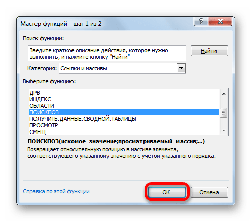
- Запускается стандартное окно Мастера функций. Переходим в нем в ту же самую группу «Ссылки и массивы». На этот раз в перечне выбираем пункт «ПОИСКПОЗ». Выполняем щелчок по кнопке «OK».
- Производится активация окошка аргументов оператора ПОИСКПОЗ. Указанная функция предназначена для того, чтобы выводить номер значения в определенном массиве по его наименованию. Именно благодаря данной возможности мы вычислим номер строки определенного значения для функции ИНДЕКС. Синтаксис ПОИСКПОЗ представлен так:
=ПОИСКПОЗ(искомое_значение;просматриваемый_массив;[тип_сопоставления])«Искомое значение» — аргумент, содержащий наименование или адрес ячейки стороннего диапазона, в которой оно находится. Именно позицию данного наименования в целевом диапазоне и следует вычислить. В нашем случае в роли первого аргумента будут выступать ссылки на ячейки на Листе 1, в которых расположены имена сотрудников.
«Просматриваемый массив» — аргумент, представляющий собой ссылку на массив, в котором выполняется поиск указанного значения для определения его позиции. У нас эту роль будет исполнять адрес столбца «Имя» на Листе 2.
«Тип сопоставления» — аргумент, являющийся необязательным, но, в отличие от предыдущего оператора, этот необязательный аргумент нам будет нужен. Он указывает на то, как будет сопоставлять оператор искомое значение с массивом. Этот аргумент может иметь одно из трех значений: -1; 0; 1. Для неупорядоченных массивов следует выбрать вариант «0». Именно данный вариант подойдет для нашего случая.
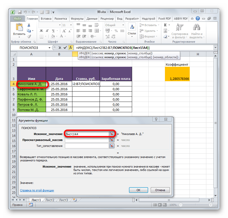
Итак, приступим к заполнению полей окна аргументов. Ставим курсор в поле «Искомое значение», кликаем по первой ячейке столбца «Имя» на Листе 1.
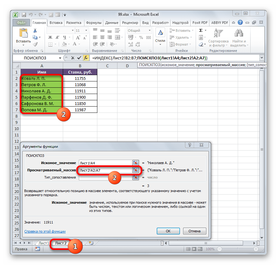
- После того, как координаты отобразились, устанавливаем курсор в поле «Просматриваемый массив» и переходим по ярлыку «Лист 2», который размещен внизу окна Excel над строкой состояния. Зажимаем левую кнопку мыши и выделяем курсором все ячейки столбца «Имя».
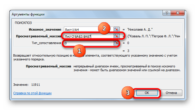
- После того, как их координаты отобразились в поле «Просматриваемый массив», переходим к полю «Тип сопоставления» и с клавиатуры устанавливаем там число «0». После этого опять возвращаемся к полю «Просматриваемый массив». Дело в том, что мы будем выполнять копирование формулы, как мы это делали в предыдущем способе. Будет происходить смещение адресов, но вот координаты просматриваемого массива нам нужно закрепить. Он не должен смещаться. Выделяем координаты курсором и жмем на функциональную клавишу F4. Как видим, перед координатами появился знак доллара, что означает то, что ссылка из относительной превратилась в абсолютную. Затем жмем на кнопку «OK».
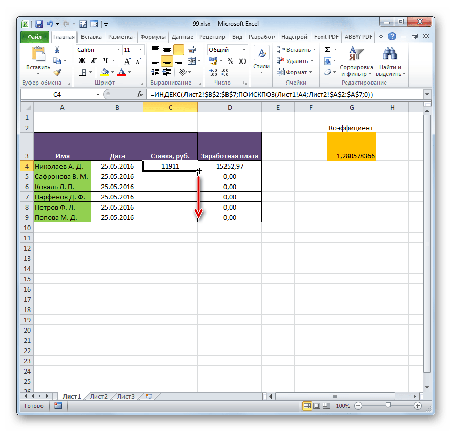
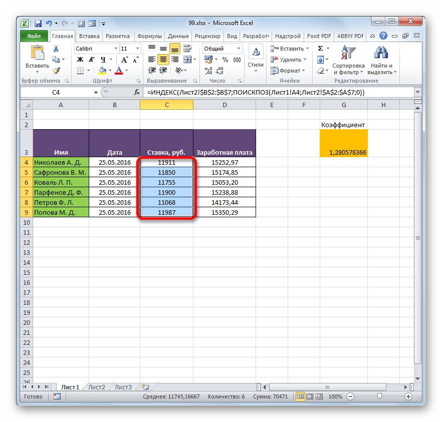
- Результат выведен на экран в первую ячейку столбца «Ставка». Но перед тем, как производить копирование, нам нужно закрепить ещё одну область, а именно первый аргумент функции ИНДЕКС. Для этого выделяем элемент колонки, который содержит формулу, и перемещаемся в строку формул. Выделяем первый аргумент оператора ИНДЕКС (B2:B7) и щелкаем по кнопке F4. Как видим, знак доллара появился около выбранных координат. Щелкаем по клавише Enter. В целом формула приняла следующий вид:
=ИНДЕКС(Лист2!$B$2:$B$7;ПОИСКПОЗ(Лист1!A4;Лист2!$A$2:$A$7;0)) - Теперь можно произвести копирование с помощью маркера заполнения. Вызываем его тем же способом, о котором мы говорили ранее, и протягиваем до конца табличного диапазона.
- Как видим, несмотря на то, что порядок строк у двух связанных таблиц не совпадает, тем не менее, все значения подтягиваются соответственно фамилиям работников. Этого удалось достичь благодаря применению сочетания операторов ИНДЕКС—ПОИСКПОЗ.


Читайте также:
Функция ИНДЕКС в Экселе
Функция ПОИСКПОЗ в Экселе
Способ 3: выполнение математических операций со связанными данными
Прямое связывание данных хорошо ещё тем, что позволяет не только выводить в одну из таблиц значения, которые отображаются в других табличных диапазонах, но и производить с ними различные математические операции (сложение, деление, вычитание, умножение и т.д.).
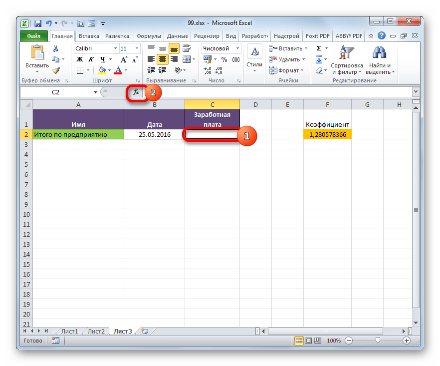
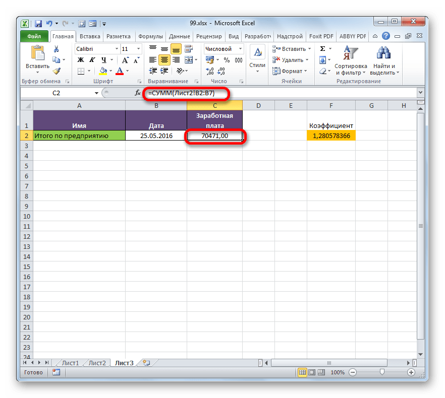
Посмотрим, как это осуществляется на практике. Сделаем так, что на Листе 3 будут выводиться общие данные заработной платы по предприятию без разбивки по сотрудникам. Для этого ставки сотрудников будут подтягиваться из Листа 2, суммироваться (при помощи функции СУММ) и умножаться на коэффициент с помощью формулы.
- Выделяем ячейку, где будет выводиться итог расчета заработной платы на Листе 3. Производим клик по кнопке «Вставить функцию».
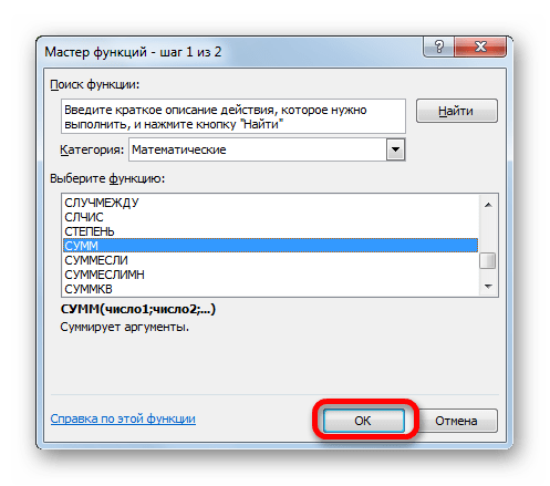
- Следует запуск окна Мастера функций. Переходим в группу «Математические» и выбираем там наименование «СУММ». Далее жмем по кнопке «OK».
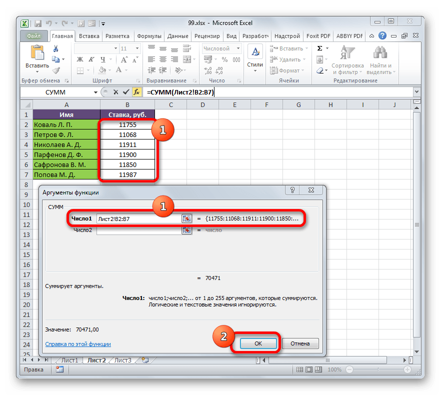
- Производится перемещение в окно аргументов функции СУММ, которая предназначена для расчета суммы выбранных чисел. Она имеет нижеуказанный синтаксис:
=СУММ(число1;число2;…)Поля в окне соответствуют аргументам указанной функции. Хотя их число может достигать 255 штук, но для нашей цели достаточно будет всего одного. Ставим курсор в поле «Число1». Кликаем по ярлыку «Лист 2» над строкой состояния.
- После того, как мы переместились в нужный раздел книги, выделяем столбец, который следует просуммировать. Делаем это курсором, зажав левую кнопку мыши. Как видим, координаты выделенной области тут же отображаются в поле окна аргументов. Затем щелкаем по кнопке «OK».
- После этого мы автоматически перемещаемся на Лист 1. Как видим, общая сумма размера ставок работников уже отображается в соответствующем элементе.
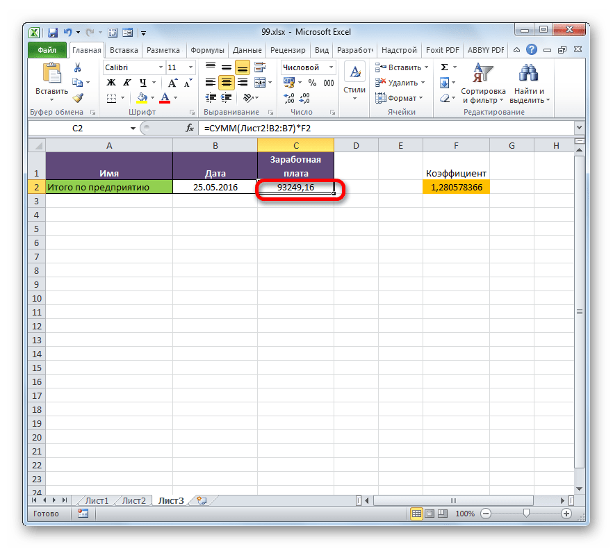
- Но это ещё не все. Как мы помним, зарплата вычисляется путем умножения величины ставки на коэффициент. Поэтому снова выделяем ячейку, в которой находится суммированная величина. После этого переходим к строке формул. Дописываем к имеющейся в ней формуле знак умножения (*), а затем щелкаем по элементу, в котором располагается показатель коэффициента. Для выполнения вычисления щелкаем по клавише Enter на клавиатуре. Как видим, программа рассчитала общую заработную плату по предприятию.
- Возвращаемся на Лист 2 и изменяем размер ставки любого работника.
- После этого опять перемещаемся на страницу с общей суммой. Как видим, из-за изменений в связанной таблице результат общей заработной платы был автоматически пересчитан.


Способ 4: специальная вставка
Связать табличные массивы в Excel можно также при помощи специальной вставки.
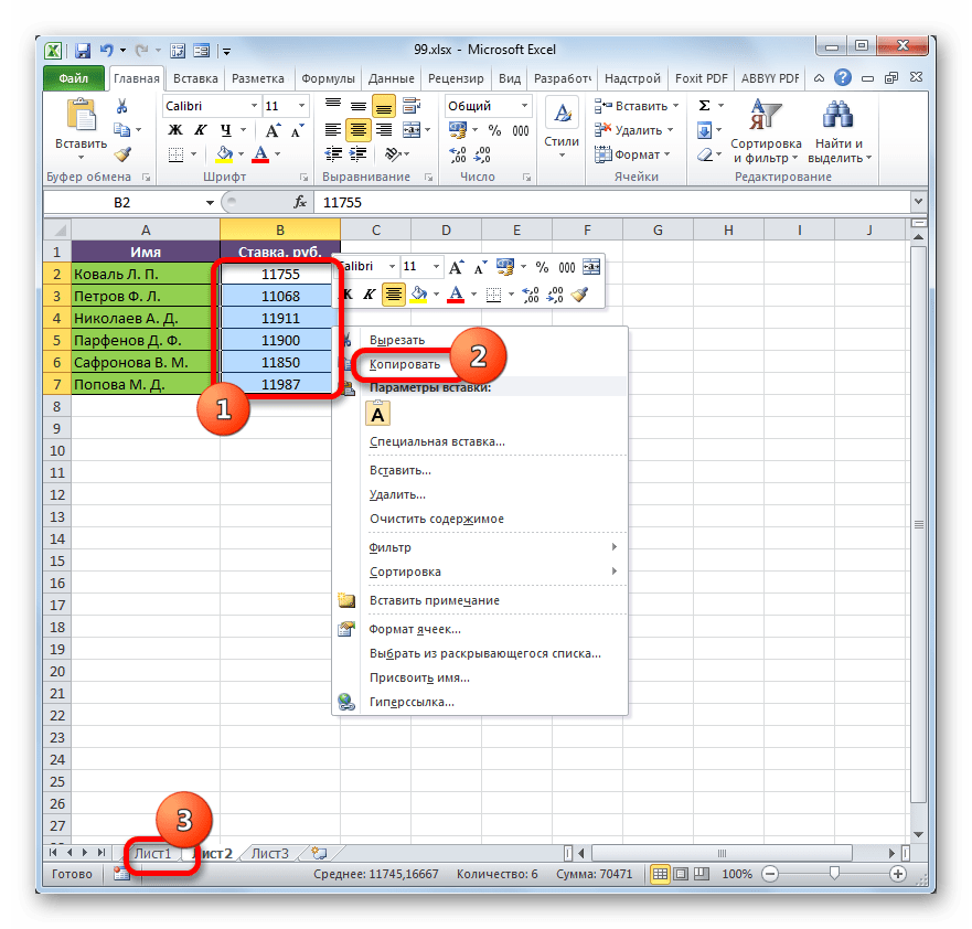
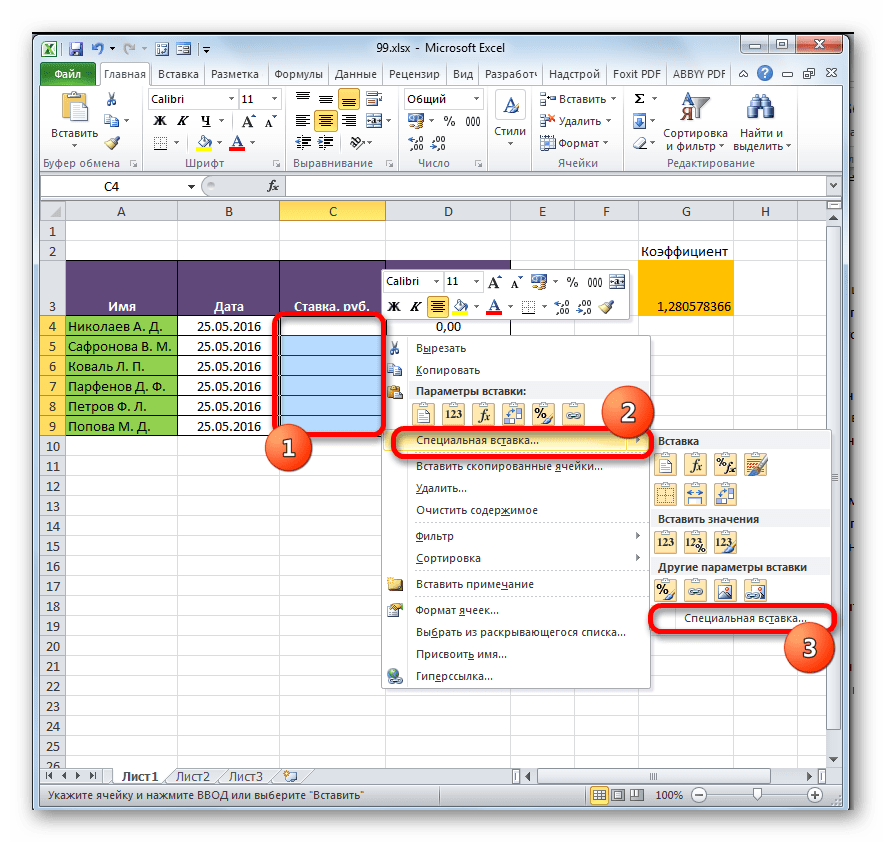
- Выделяем значения, которые нужно будет «затянуть» в другую таблицу. В нашем случае это диапазон столбца «Ставка» на Листе 2. Кликаем по выделенному фрагменту правой кнопкой мыши. В открывшемся списке выбираем пункт «Копировать». Альтернативной комбинацией является сочетание клавиш Ctrl+C. После этого перемещаемся на Лист 1.
- Переместившись в нужную нам область книги, выделяем ячейки, в которые нужно будет подтягивать значения. В нашем случае это столбец «Ставка». Щелкаем по выделенному фрагменту правой кнопкой мыши. В контекстном меню в блоке инструментов «Параметры вставки» щелкаем по пиктограмме «Вставить связь».

Существует также альтернативный вариант. Он, кстати, является единственным для более старых версий Excel. В контекстном меню наводим курсор на пункт «Специальная вставка». В открывшемся дополнительном меню выбираем позицию с одноименным названием.
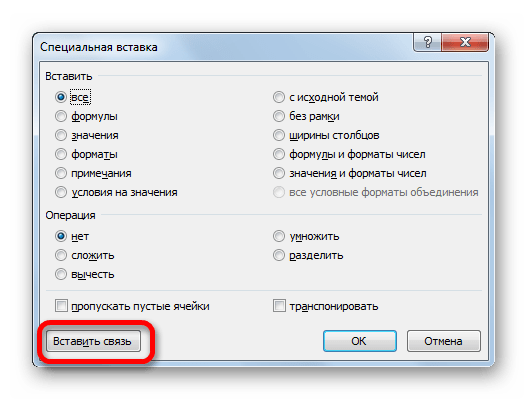
- После этого открывается окно специальной вставки. Жмем на кнопку «Вставить связь» в нижнем левом углу ячейки.
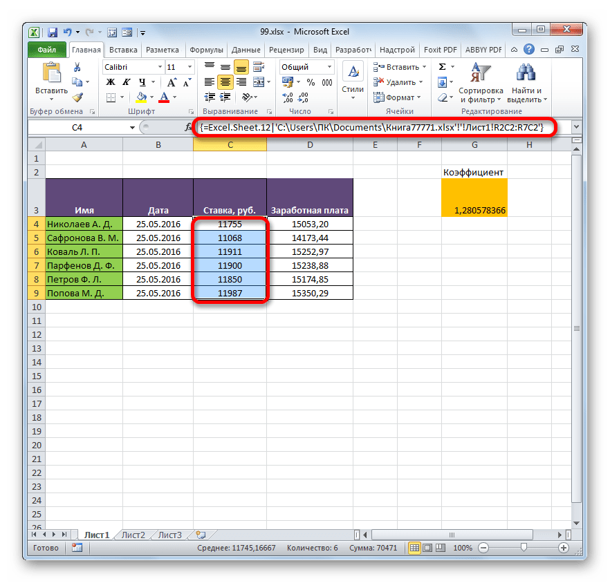
- Какой бы вариант вы не выбрали, значения из одного табличного массива будут вставлены в другой. При изменении данных в исходнике они также автоматически будут изменяться и во вставленном диапазоне.


Урок: Специальная вставка в Экселе
Способ 5: связь между таблицами в нескольких книгах
Кроме того, можно организовать связь между табличными областями в разных книгах. При этом используется инструмент специальной вставки. Действия будут абсолютно аналогичными тем, которые мы рассматривали в предыдущем способе, за исключением того, что производить навигацию во время внесений формул придется не между областями одной книги, а между файлами. Естественно, что все связанные книги при этом должны быть открыты.
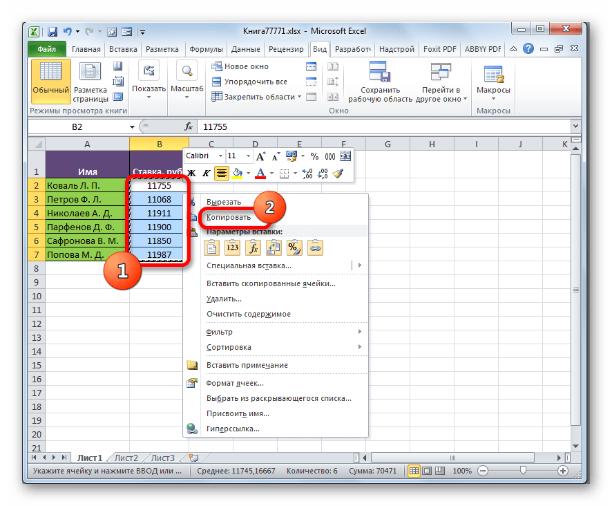
- Выделяем диапазон данных, который нужно перенести в другую книгу. Щелкаем по нему правой кнопкой мыши и выбираем в открывшемся меню позицию «Копировать».
- Затем перемещаемся к той книге, в которую эти данные нужно будет вставить. Выделяем нужный диапазон. Кликаем правой кнопкой мыши. В контекстном меню в группе «Параметры вставки» выбираем пункт «Вставить связь».
- После этого значения будут вставлены. При изменении данных в исходной книге табличный массив из рабочей книги будет их подтягивать автоматически. Причем совсем не обязательно, чтобы для этого были открыты обе книги. Достаточно открыть одну только рабочую книгу, и она автоматически подтянет данные из закрытого связанного документа, если в нем ранее были проведены изменения.

Но нужно отметить, что в этом случае вставка будет произведена в виде неизменяемого массива. При попытке изменить любую ячейку со вставленными данными будет всплывать сообщение, информирующее о невозможности сделать это.

Изменения в таком массиве, связанном с другой книгой, можно произвести только разорвав связь.
Разрыв связи между таблицами
Иногда требуется разорвать связь между табличными диапазонами. Причиной этого может быть, как вышеописанный случай, когда требуется изменить массив, вставленный из другой книги, так и просто нежелание пользователя, чтобы данные в одной таблице автоматически обновлялись из другой.
Способ 1: разрыв связи между книгами
Разорвать связь между книгами во всех ячейках можно, выполнив фактически одну операцию. При этом данные в ячейках останутся, но они уже будут представлять собой статические не обновляемые значения, которые никак не зависят от других документов.
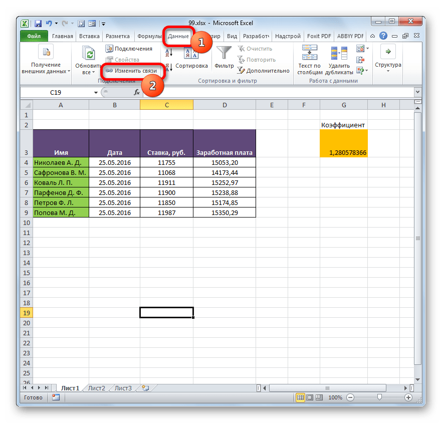
- В книге, в которой подтягиваются значения из других файлов, переходим во вкладку «Данные». Щелкаем по значку «Изменить связи», который расположен на ленте в блоке инструментов «Подключения». Нужно отметить, что если текущая книга не содержит связей с другими файлами, то эта кнопка является неактивной.
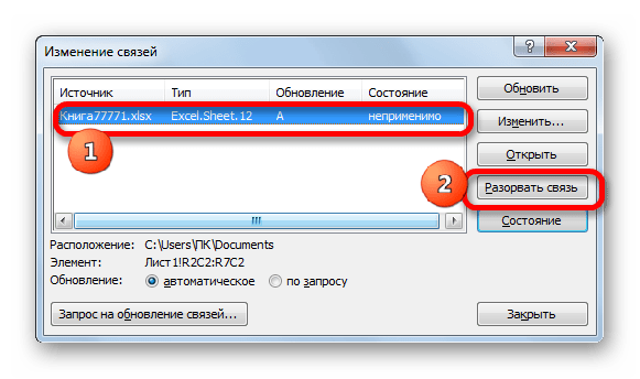
- Запускается окно изменения связей. Выбираем из списка связанных книг (если их несколько) тот файл, с которым хотим разорвать связь. Щелкаем по кнопке «Разорвать связь».
- Открывается информационное окошко, в котором находится предупреждение о последствиях дальнейших действий. Если вы уверены в том, что собираетесь делать, то жмите на кнопку «Разорвать связи».
- После этого все ссылки на указанный файл в текущем документе будут заменены на статические значения.


Способ 2: вставка значений
Но вышеперечисленный способ подходит только в том случае, если нужно полностью разорвать все связи между двумя книгами. Что же делать, если требуется разъединить связанные таблицы, находящиеся в пределах одного файла? Сделать это можно, скопировав данные, а затем вставив на то же место, как значения. Кстати, этим же способом можно проводить разрыв связи между отдельными диапазонами данных различных книг без разрыва общей связи между файлами. Посмотрим, как этот метод работает на практике.
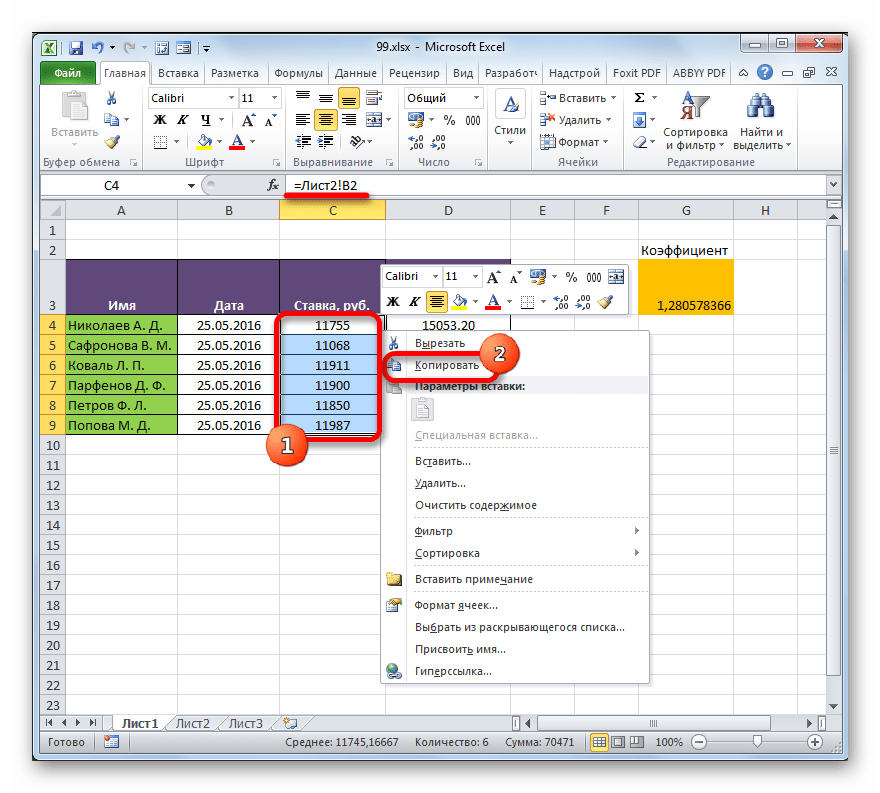
- Выделяем диапазон, в котором желаем удалить связь с другой таблицей. Щелкаем по нему правой кнопкой мыши. В раскрывшемся меню выбираем пункт «Копировать». Вместо указанных действий можно набрать альтернативную комбинацию горячих клавиш Ctrl+C.
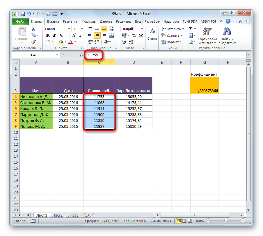
- Далее, не снимая выделения с того же фрагмента, опять кликаем по нему правой кнопкой мыши. На этот раз в списке действий щелкаем по иконке «Значения», которая размещена в группе инструментов «Параметры вставки».
- После этого все ссылки в выделенном диапазоне будут заменены на статические значения.

Как видим, в Excel имеются способы и инструменты, чтобы связать несколько таблиц между собой. При этом, табличные данные могут находиться на других листах и даже в разных книгах. При необходимости эту связь можно легко разорвать.
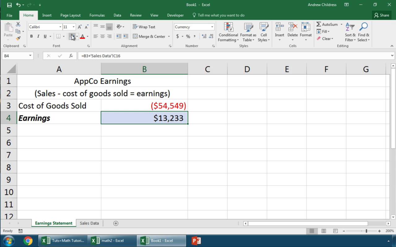
As you use and build more Excel workbooks, you’ll need to link them up. Maybe you want to write formulas that use data between different sheets in a workbook. You can even write formulas that use data from multiple different workbooks.
If I want to keep my files clean and tidy, I’ve found it’s best to separate large sheets of data from the formulas that summarize them. I often use a single workbook or sheet to summarize things.
In this tutorial, you’ll learn how to link data in Excel. First, we’ll learn how to link up data in the same workbook on different sheets. Then, we’ll move on to linking up multiple Excel workbooks to import and sync data between files.
How to Quickly Link Data in Excel Workbooks (Watch & Learn)
I’ll walk you through two examples linking up your spreadsheets. You’ll see how to pull data from another workbook in Excel and keep two workbooks connected. We’ll also walk through a basic example to write formulas between sheets in the same workbook.
Let’s walk through an illustrated guide to linking up your data between sheets and workbooks in Excel.
Basics: How to Link Between Sheets in Excel
Let’s start off by learning how to write formulas using data from another sheet. You probably already know that Excel workbooks can contain multiple worksheets. Each worksheet is a tab of its own, and you can switch tabs by clicking on them at the bottom of Excel.
Complex workbooks can easily grow to many sheets. In time, you’ll certainly need to write formulas to work with data on different tabs.
Maybe you use a single sheet in your workbook for all of your formulas to summarize your data, and separate sheets to hold the original data.

Let’s learn how to write a multi-sheet formula to work with data from multiple sheets in the same workbook.
1. Start a New Formula in Excel
Most formulas in Excel start off with the equals (=) sign. Double click or start typing in a cell and begin writing the formula that you want to link up. For my example, I’ll write a sum formula to add up several cells.
I’ll open up the = sign, and then click on the first cell on my current sheet to make it the first part of the formula. Then, I’ll type a + sign to add my second cell to this formula.
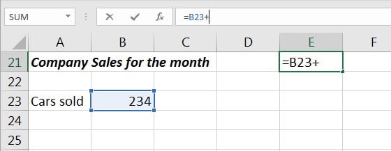

Now, make sure that you don’t close out your formula and press enter yet! You’ll want to leave the formula open before you switch sheets.
2. Switch Sheets in Excel
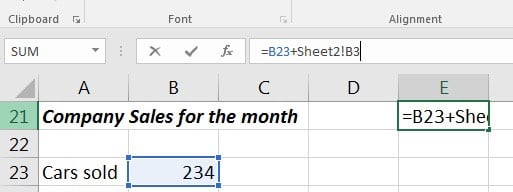
While you still have the formula open, click on a different sheet tab at the bottom of Excel. It’s very important that you don’t close out the formula before you click on the next cell to include as part of the formula.

After you switch sheets, click on the next cell that you want to include in the formula. As you can see in the screenshot below, Excel automatically writes the part of the formula that references a cell on another sheet for you.
Notice in the screenshot below that to reference a cell on another sheet, Excel adds «Sheet2!B3», which simply references cell B3 on a sheet named Sheet2. You could write this manually, but clicking on the cells makes Excel write it for you automatically.

3. Finish the Excel Formula
At this point, you can press enter to close out and complete your multi-sheet formula. When you do so, Excel will jump back to where you started the formula and show you the results.
You could also keep writing the formula, including cells from more sheets and other cells on the same sheet. Keep combining those references throughout the workbook for all the data you need.
Level Up: How to Link Multiple Excel Workbooks
Let’s learn how to pull data from another workbook. With this skill, you can write formulas that pull together data from entirely separate Excel workbooks.
For this section of the tutorial, you can use two workbooks that you can download for free as a part of this tutorial. Open them both up in Excel, and follow the directions below.
1. Open Both Workbooks
Let’s start off by writing a formula that includes data from two different workbooks.
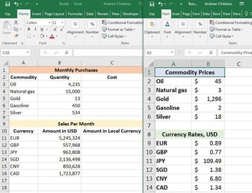
The easiest way to use this feature is to open up two Excel workbooks at the same time and put them side by side. I use the Windows Snap feature to split them to each take up half the screen. You need to keep both workbooks in view to write formulas between them.
In the screenshot below, I’ve opened two workbooks that I’ll write formulas for side-by-side. For my example, I’m running a business that buys a variety of products, and sells them in a variety of countries. So, I’ll use separate workbooks to track my purchases/sales and cost data.
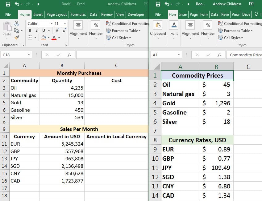

2. Start Writing Your Formula in Excel
The price of what I buy can change, and so can the rate that I receive payments in. I need to keep a lookup list of rates and multiply it times my purchases. This is the perfect time to link two workbooks together and write formulas between them.
Let’s take the number of barrels of oil I buy each month times the price per barrel. In the first Cost cell (cell C3), I’ll start writing a formula by typing the equals sign (=), and then clicking on cell B3 to grab the quantity. Now, I’ll add an * to prepare to multiply the quantity by the rate.
So far, your formula should be:
=B3*


Don’t close out your formula yet. Make sure to leave it open before moving onto the next step; we still need to point Excel to the price data to multiply the quantity by.
3. Switch Excel Workbooks
It’s time to switch workbooks, and this is why it’s important to keep both of your datasets in view while working between workbooks.
With your formula still open, click over to the other workbook. Then, click on a cell in your second workbook to link up the two Excel files.


Excel automatically wrote the reference to a separate workbook as part of the cell formula:
=B3*[Prices.xlsx]Sheet1!$B$2
Once you press Enter, Excel will calculate the final cost by multiplying the quantity in the first workbook times the price in the second workbook.
Now, keep working on your Excel skills by multiplying each of the quantities or values times the reference amounts in the «Prices» workbook.
In short, the key is to get your workbooks open side by side, and simply switch workbooks to write formulas referencing other files.
There’s nothing stopping you from linking up more than two workbooks. You could open many workbooks to link up and write formulas, connecting the data between many sheets to keep cells up to date.
How to Refresh Your Data Between Workbooks
When you’ve written formulas that reference other Excel workbooks, you’ll need to think about how you’ll update your data.
So, what happens when the data changes in the workbook that you’re linking to? Will your workbook automatically update, or will you need to refresh your files to pull over the last data and import it?
The answer is, «it depends», and specifically, it depends upon if both workbooks are still open at the same time.
Example 1: Both Excel Workbooks Still Open
Let’s check out an example using the same workbook from the prior step. Both workbooks are still open. Let’s see what happens when we change the price of oil from $45 per barrel to $75 per barrel:


In the screenshot above, you can see that when we updated the price of oil, the other workbook automatically updated.
This is important to know: if both workbooks are open at the same time, changes will update automatically and in real-time. When you change one variable, the other workbook will update or recalculate based upon the new value.
Example 2: With One Workbook Closed
What if you only open one workbook at a time? For example, each morning, we update prices of our commodities and currencies, and in the evening we review the impact of the change to our purchases and sales.
The next time you open up your workbook that references other sheets, you might get a message similar to the one below. You can click on Update to pull in the latest data from your reference workbook.
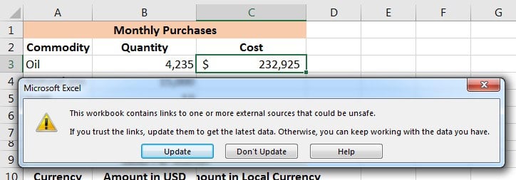


You might also see a menu where you can click Enable Content to automate updating data between Excel files.
Recap and Keep Learning More About Excel
Writing formulas between sheets and workbooks is a necessary skill when you work with Microsoft Excel. Using multiple spreadsheets inside your formulas is no problem with a bit of know-how.
Check out these additional tutorials to learn more about Excel skills and how to work with data. These tutorials are a great way to continue learning Excel.
Let me know in the comments if you have any questions about how to link up your Excel workbooks.
Did you find this post useful?

I believe that life is too short to do just one thing. In college, I studied Accounting and Finance but continue to scratch my creative itch with my work for Envato Tuts+ and other clients. By day, I enjoy my career in corporate finance, using data and analysis to make decisions.
I cover a variety of topics for Tuts+, including photo editing software like Adobe Lightroom, PowerPoint, Keynote, and more. What I enjoy most is teaching people to use software to solve everyday problems, excel in their career, and complete work efficiently. Feel free to reach out to me on my website.
Excel files are also called workbooks for a very good reason. They can have multiple sheets, or worksheets, to help you organize your data. When working with multiple sheets, you may need to have links between them so that values in one sheet can be used in another.
In this article, we’ll explain how to link data between worksheets in Excel. You’ll see several examples on linking sheets in the same workbook as well as across different ones.
Why link data between sheets in Excel?
Linking sheets in Excel can be a great way to organize your data and keep them consistent across different worksheets. You may want to do this for different purposes, for example:
- You have a workbook containing data split by month, by state, or by salesperson, and you want a summary in one of the sheets.
- You want to create lists using links from different sheets in Excel.
- You want to collect data from multiple sheets and combine them into one to create a master sheet. Or, you may want to link data from a master sheet so that your data in other sheets are always up-to-date.
- Your data is growing and becoming too voluminous. As a result, you split it into different workbooks to be managed by different people. There can be times when you need to write formulas to get data out of these files.
Creating links between sheets is pretty easy to do. Besides, the main benefit is that whenever your data in the source sheet changes, the data in the destination sheet will be automatically updated as well.
Problems with linking large data between worksheets in the same or different Excel workbooks
Indeed, using multiple worksheets can certainly make your data in one workbook easier to manage. However, linking large amounts of data between worksheets could decrease the performance of your Excel workbook. Avoid inter-workbook links unless it’s absolutely necessary because they can be slow, easily broken, and not always easy to find and fix.
We suggest you try another solution 👇
When getting large data from different worksheets, especially from different workbooks, we recommend that you import instead of linking. Linking will slow down your Excel file, while an optimized performance can be maintained if you simply import data from Excel to Excel. Use a tool such as Coupler.io to refresh your data on the schedule you want to keep your data up-to-date.

To start using Coupler.io, sign up for a free account and create your first importer. A wizard will walk you through setting up the source, destination, and auto-refresh schedule for your importer. If you’re importing from Excel to Excel, choose Microsoft Excel as the source and destination of your importer, as follows:
#1. Set up a source
Select Microsoft Excel as the source that contains your data. You’ll need to connect to your Microsoft account and select the workbook and worksheet(s) you want to import. If you want, you can import only a selected range from your worksheets, e.g., range B3:G10 only.

Notice that with Coupler.io, you can also import data from different sources such as HubSpot, Jira, QuickBooks, and more. Check out the complete list of Coupler.io integrations with Excel.
#2. Set up a destination
For the destination, select Microsoft Excel. No need to connect again if you’re importing to the same Microsoft account. After that, choose the workbook and worksheet where you want your data imported.

#3. Schedule
You can keep your data up-to-date by setting up an automatic data refresh on the schedule you want.

Finally, click Save and Run to run your first importer. The import process may take several seconds or minutes to complete.
How to link two Excel sheets in the same workbook
Now, let’s see how to link two sheets in the same Excel workbook, including some tips and examples.
How to link sheets in Excel with a formula
To refer to a cell or range in another worksheet in the same workbook, type the name of the source worksheet followed by an exclamation mark (!) before the range address—see the following examples:
- To reference a single cell A1 in Sheet2:
=Sheet2!A1
- To reference a single cell A1 but the sheet name contains spaces:
='Sheet 2'!A1
- To reference a range of cells A1 to C10 in Sheet2:
=Sheet2!A1:C10
- To reference column A in Sheet2:
=Sheet2!A:A
- To reference multiple columns A to E in Sheet2:
=Sheet2!A:E
- To reference row 5 in Sheet2:
=Sheet2!5:5
- To reference multiple rows 1 to 5 in Sheet2:
=Sheet2!1:5
- To reference a worksheet-level named range Data in Sheet2:
=Sheet2!Data
- To reference a workbook-level named range Data in Sheet2:
=Data
You can always manually type the linking formula in a destination cell. However, doing that is not recommended because it typically leads to mistakes. So, instead of typing the formula manually, check the tips below.
Tip 1: Create a link from the destination sheet
With the following spreadsheet, suppose you want to show the total for New York in the Summary sheet. In cell B2 of the Summary sheet, you want to display the values of cell F5 from the New York sheet.
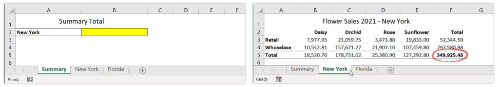
To do that, follow the steps below:
- Begin by opening the destination sheet (Summary).
- Type = (equal sign) in the destination cell (B2).

- Switch to source sheet (New York).
- Select the cell you want to link (F5), then press Enter.

As a result, when you click on the destination cell, you’ll see the following formula:
='New York'!F5

Notice that Excel automatically encloses the sheet name with single quotation marks because there is a space character in the sheet name.
Tip 2: Use Copy and Paste Link
This second tip also allows you to link to another sheet without manually typing the linking formula. Unlike the first method that begins from the destination sheet, this method starts from the source sheet.
This time, suppose you want to show the total for Florida in the Summary sheet. In cell B3 of the Summary sheet, you want to display the values of cell F5 from the Florida sheet.

Follow the steps below:
- Begin by opening the source sheet (Florida).
- Right-click on the cell you want to link (F5), then select Copy.
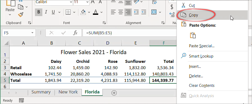
- Switch to the destination sheet (Summary).
- In the destination cell (B3), right-click and select Paste Link.

As a result, when you click on B3, you’ll see the following formula:
=Florida!$F$5

Notice that by default, this method returns an absolute reference. If you want to change it to a relative reference, simply highlight the formula and press F4 multiple times to remove the dollar signs.
How to link numbers from different sheets in Excel using the INDIRECT function
In the previous example, notice that the New York and Florida sheets have the same layout. In cases like this, you can also use the INDIRECT function in the formula to get the totals.
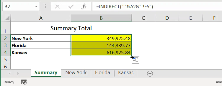
Now, let’s see the following spreadsheet with a Summary sheet and three other sheets with a similar layout. Assume you want to link the total in cell F5 from the three sheets and put them in the Summary sheet using the INDIRECT function.

To do that, follow the steps below:
- Link the total for New York only:
='New York'!F5

- Replace the formula using the INDIRECT function below. Notice that we concatenate A2 with single quotes because its value contains a space character.
=INDIRECT("'"&A2&"'!F5")

- Drag the formula down to A4 to apply it to the other states.
How to link data in a range of cells between sheets in Excel
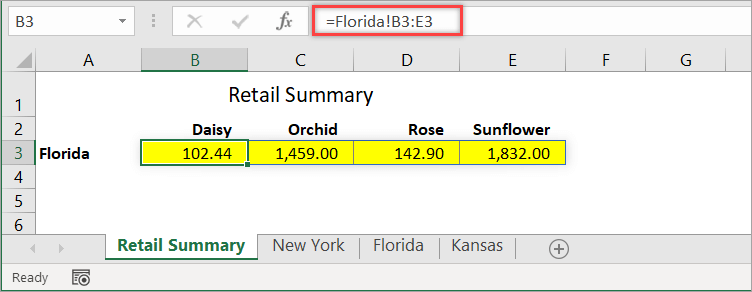
With the following spreadsheet, suppose you want to link the retail sales data for Florida and put them in the Retail Summary sheet, as the following screenshot shows:

The range to link is in B3:E3 of the second sheet. To display it in the destination sheet, use the following formula in a cell:
=Florida!B3:E3
How to link columns from different sheets to another sheet in Excel
With the following spreadsheet, suppose you want to link the entire Column B from the Product sheet to Sheet1. To do that, you can use the following formula:
=Product!B:B

However, if you notice, the blank cells are showing zeros. If you want to see empty cells when there is nothing in the original sheet, you can change the formula to the one below:
=IF(LEN(Product!B:B)>0, Product!B:B,"")

How to link to a defined name in other sheets in Excel
For most people, words are easier to remember than numbers or codes. For this reason, Excel allows you to name an individual cell or range of cells. Then, you can use these names when referring to data in another sheet instead of typing the range address.
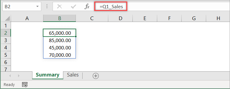
With the following worksheet, let’s create a defined name for range B2:B5 and name it Q1_Sales.
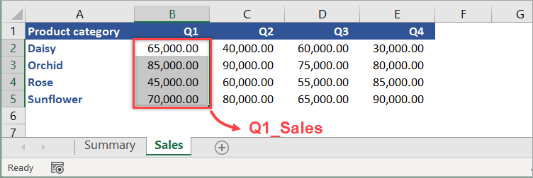
First, select the range of cells to include (B2:B5). Then, in the Name Box, type Q1_Sales and press Enter — and Done!

By default, Excel creates the name at the workbook level. To reference the defined name in another worksheet, just type the following formula into any cell.
=Q1_Sales
You can also use the defined name with an Excel function in a formula. For example, the following formula calculates the average of Q1_Sales:
=AVERAGE(Q1_Sales)

How to link lists in different sheets in Excel
With the following spreadsheet, suppose you want to create a dropdown list in Sheet1 that contains product category data from Sheet2. This will allow you to select the Category in Column D using a dropdown instead of typing it manually.

Follow these steps:
- In Sheet1, select the range you want to apply to the dropdown list, which is D2:D4.
- Click Data > Data Validation.
- In the “Data Validation” dialog box, enter the following details, then click OK.
- Allow :
List - Source :
=Sheet2!$A$2:$A$5

We enter a link reference to product category data in Sheet2, which is in range A2:A5. As a result, now you select the product category in Sheet1 using a dropdown, as shown below:

How to link to hidden sheets in Excel
A sheet can be hidden for different reasons. For example, you may want to hide sheets that are no longer frequently being used by other users.
To create a link to a hidden sheet, simply unhide it first, create the link, then hide it again if necessary.
You can actually refer to hidden sheets without unhiding them first, as long as you know the name of the sheets and the range you want to link from these sheets. However, most of the time, you’ll need to unhide them first to see the data you want to link so that you don’t accidentally refer to the wrong range of cells when creating the links.
There are two different types of hidden sheets in Excel: hidden and very hidden. While unhiding a hidden sheet is very easy, you will need to open the Visual Basic Editor (VBE) to unhide a very hidden sheet.
To link to a hidden sheet in Excel
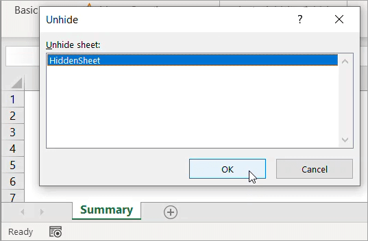
- Unhide the sheet by right-clicking on any visible sheet, then select Unhide.

- In the “Unhide” dialog box that appears, select the sheet you want to unhide, then click OK.
- Use a linking formula to link the data you want to show in another sheet.
For example, the following formula in the Summary sheet shows the range A1:E1 from the sheet we just made visible.
=HiddenSheet!A1:E1

- If you want, hide the sheet again by clicking on the sheet tab, then select Hide.

To link to a very hidden sheet in Excel
- Open the VBE by pressing Alt+F11.
- Press F4 or click View > Properties Window to open the Properties window under the Project Explorer if it’s not already open.
- In Project Explorer, select the very hidden sheet you want to unhide. Then, set its Visible property to
-1 - xlSheetVisiblein the Properties window.

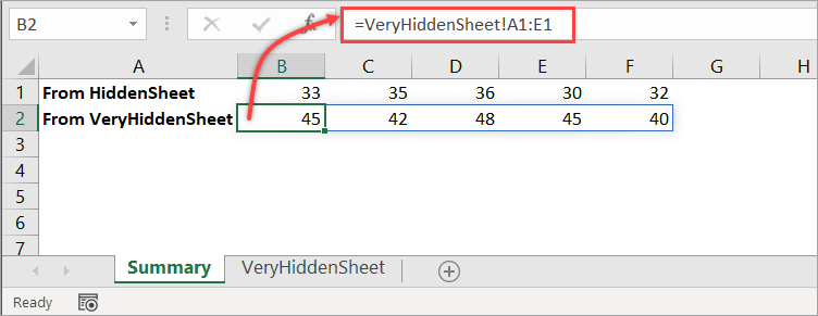
- Use a linking formula to link the data you want to show in another sheet. For example, the following formula in the Summary sheet shows the range A1:E1 from the very hidden sheet we just made visible.
=VeryHiddenSheet!A1:E1
- If you want, change the sheet’s Visible property back to
2 - xlSheetVeryHiddenin the Properties window to make it a very hidden sheet again.
How to link sheets in Excel to a master sheet
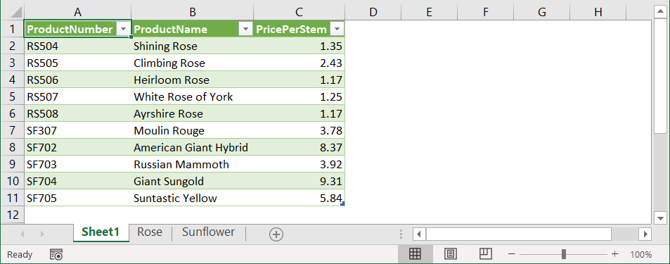
With the following spreadsheet, suppose you want to link data from two worksheets into one.

Notice that it’s like combining two ranges, which are Rose!A1:C6 and Sunflower!A1:C6.
However, combining ranges in Excel using a formula is a bit complex. An easier way to do this is using Power Query, as explained in the steps below:
- In the Rose sheet, select the range A1:C6.
- Then, on the Data tab in the Get & Transform Data section, click From Table/Range.
- In the “Create Table” dialog box, ensure that the My table has headers option checked.

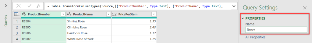
- Click OK — this will bring you to the Power Query editor.
- In the Query Settings, give your query a descriptive name, e.g., Roses.
- Click the Home tab, then click Close & Load > Close & Load To…
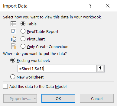
- In the “Import Data” dialog box, select Only Create Connection, then press OK.

- Repeat steps 1-7 for the Sunflower data. But for the fifth step, let’s rename the query as Sunflowers.
- Re-launch the Power Query editor by clicking the Data tab, then click Get Data > Launch Power Query Editor…
- Select any query, then click Append Queries > Append Queries as New to keep the existing queries unchanged.

- In the Append window, select the other table as the second table, then click OK.

- Make sure to select the newly created query. Then, on the Home tab, click Close & Load > Close & Load To…
- In the “Import Data” dialog box, load the combined data to Sheet1!A1, then click OK.
To see the result, click Sheet1. You’ll find the combined data as shown in the following screenshot:
When the source data from the other sheets change, you won’t see the new changes right away. Using this method, you need to click the Refresh All button in the Data tab to see the latest data.
How to link two Excel sheets in different workbooks
To link to a worksheet in another workbook, you can do it whether the source file is open or closed. If possible, we suggest you open all the source workbooks first before creating the links in the destination workbook. Why? Because this way is easier.
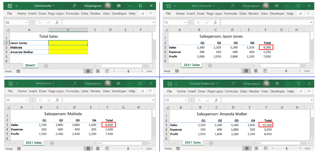
As an example, suppose you have the following four workbooks: Summary.xlsx, Jason Jones.xlsx, Melinda.xlsx, and Amanda Walker.xlsx. In the Summary workbook, you want to link the total sales of each salesperson, which is in cell F3 of each of the other workbooks—see the following screenshot:
Link to another worksheet when the source workbook is open
When all the source files are open, you can follow the steps below to create the links:
- In the Summary workbook, type = (equal sign) in the destination cell for Jason Jones.

- Click View > Switch Windows, then select Jason Jones.xlsx to switch to this workbook.

- Select the cell to link, in this case, F3, then press Enter.

- Repeat Steps 1-3 for Melinda and Amanda Walker.
As the final result, you’ll see formulas with the following format when you click on each of the destination cells:
='[SourceWorkbook.xlsx]SheetName'!RangeAddress

Note: In the above example, the workbook name and/or sheet name contain spaces, so the path is enclosed in single quotation marks.
Link to another worksheet when the source workbook is closed
If you close the source workbooks one by one, the linking formulas in the Summary workbook will change as shown in the below screenshot:
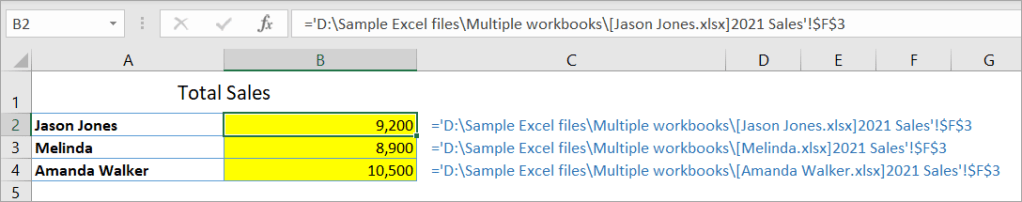
Now, you get the idea — you need to use the full path when linking to a workbook that’s currently closed.
Basically, you can use the following format to link data from any Excel workbooks:
='FolderPath[SourceWorkbook.xlsx]SheetName'!RangeAddress
However, if possible, just open the source files before you create the link, so you don’t need to manually type the long formula that’s shown above. 🙂
Can you break links between sheets in different workbooks in Excel?
When you open an Excel file, there may be formulas in it that get data from another workbook.
To locate these formulas, click on the Data tab in the ribbon. If the Edit Links button is available, it means that your file contains links to other workbooks.

To break a link, follow these steps:
- On the Data tab, in the Queries & Connections section, click Edit Links.
- In the “Edit Links” dialog box that appears, select the link you want to break and click Break Link.

- Click Break Links in the confirmation dialog box that appears.

Notice that when you break a link to the source workbook, all the linking formulas are converted to their current values. This action cannot be undone, so you may want to back up your workbook before breaking any links.
- Click Close.
In this section, you’ve learned the basics of how to link sheets from different workbooks, as well as how to break those links. If you’re interested in more examples of linking worksheets from different workbooks, check out our article on how to link Excel files.
Thanks for reading, and good luck with your data!
-

Senior analyst programmer

Back to Blog
Focus on your business
goals while we take care of your data!
Try Coupler.io