
Содержание
- Create an external reference (link) to a cell range in another workbook
- Create an external reference between cells in different workbooks
- Create a link to a worksheet in the same workbook
- Need more help?
- Link Cells Between Sheets and Workbooks In Excel
- Why Link Cell Data in Excel
- How to Link Two Single Cells
- How to Link a Range of Cells
- How to Link a Cell With a Function
- How to Link Cells From Different Excel Files
- Become a Pro Microsoft Excel User
Create an external reference (link) to a cell range in another workbook
You can refer to the contents of cells in another workbook by creating an external reference formula. An external reference (also called a link) is a reference to a cell or range on a worksheet in another Excel workbook, or a reference to a defined name in another workbook.
Open the workbook that will contain the external reference (the destination workbook) and the workbook that contains the data that you want to link to (the source workbook).
Select the cell or cells where you want to create the external reference.
Type = (equal sign).
If you want to use a function, such as SUM, then type the function name followed by an opening parenthesis. For example, =SUM(.
Switch to the source workbook, and then click the worksheet that contains the cells that you want to link.
Select the cell or cells that you want to link to and press Enter.
Note: If you select multiple cells, like =[SourceWorkbook.xlsx]Sheet1!$A$1:$A$10, and have a current version of Microsoft 365, then you can simply press ENTER to confirm the formula as a dynamic array formula. Otherwise, the formula must be entered as a legacy array formula by pressing CTRL+SHIFT+ENTER. For more information on array formulas, see Guidelines and examples of array formulas.
Excel will return you to the destination workbook and display the values from the source workbook.
Note that Excel will return the link with absolute references, so if you want to copy the formula to other cells, you’ll need to remove the dollar ($) signs:
=[SourceWorkbook.xlsx]Sheet1! $A $1
If you close the source workbook, Excel will automatically append the file path to the formula:
Open the workbook that will contain the external reference (the destination workbook) and the workbook that contains the data that you want to link to (the source workbook).
Select the cell or cells where you want to create the external reference.
Type = (equal sign).
Switch to the source workbook, and then click the worksheet that contains the cells that you want to link.
Press F3, select the name that you want to link to and press Enter.
Note: If the named range references multiple cells, and you have a current version of Microsoft 365, then you can simply press ENTER to confirm the formula as a dynamic array formula. Otherwise, the formula must be entered as a legacy array formula by pressing CTRL+SHIFT+ENTER. For more information on array formulas, see Guidelines and examples of array formulas.
Excel will return you to the destination workbook and display the values from the named range in the source workbook.
Open the destination workbook and the source workbook.
In the destination workbook, Go to Formulas > Defined Names > Define Name.
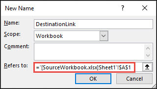
In the New Name dialog box, in the Name box, type a name for the range.
In the Refers to box, delete the contents, and then keep the cursor in the box.
If you want the name to use a function, enter the function name, and then position the cursor where you want the external reference. For example, type =SUM(), and then position the cursor between the parentheses.
Switch to the source workbook, and then click the worksheet that contains the cells that you want to link.
Select the cell or range of cells that you want to link, and click OK.
 Defined Names > Define Name > New Name.» loading=»lazy»>
External references are especially useful when it’s not practical to keep large worksheet models together in the same workbook.
Merge data from several workbooks You can link workbooks from several users or departments and then integrate the pertinent data into a summary workbook. That way, when the source workbooks are changed, you won’t have to manually change the summary workbook.
Create different views of your data You can enter all of your data into one or more source workbooks, and then create a report workbook that contains external references to only the pertinent data.
Streamline large, complex models By breaking down a complicated model into a series of interdependent workbooks, you can work on the model without opening all of its related sheets. Smaller workbooks are easier to change, don’t require as much memory, and are faster to open, save, and calculate.
Formulas with external references to other workbooks are displayed in two ways, depending on whether the source workbook — the one that supplies data to a formula — is open or closed.
When the source is open, the external reference includes the workbook name in square brackets ( [ ]), followed by the worksheet name, an exclamation point ( !), and the cells that the formula depends on. For example, the following formula adds the cells C10:C25 from the workbook named Budget.xls.
When the source is not open, the external reference includes the entire path.
Note: If the name of the other worksheet or workbook contains spaces or non-alphabetical characters, you must enclose the name (or the path) within single quotation marks as in the example above. Excel will automatically add these for you when you select the source range.
Formulas that link to a defined name in another workbook use the workbook name followed by an exclamation point (!) and the name. For example, the following formula adds the cells in the range named Sales from the workbook named Budget.xlsx.
Select the cell or cells where you want to create the external reference.
Type = (equal sign).
If you want to use a function, such as SUM, then type the function name followed by an opening parenthesis. For example, =SUM(.
Switch to the worksheet that contains the cells that you want to link to.
Select the cell or cells that you want to link to and press Enter.
Note: If you select multiple cells (=Sheet1!A1:A10), and have a current version of Microsoft 365, then you can simply press ENTER to confirm the formula as a dynamic array formula. Otherwise, the formula must be entered as a legacy array formula by pressing CTRL+SHIFT+ENTER. For more information on array formulas, see Guidelines and examples of array formulas.
Excel will return to the original worksheet and display the values from the source worksheet.
Create an external reference between cells in different workbooks
Open the workbook that will contain the external reference (the destination workbook, also called the formula workbook) and the workbook that contains the data that you want to link to (the source workbook, also called the data workbook).
In the source workbook, select the cell or cells you want to link.
Press Ctrl+C or go to Home > Clipboard > Copy.
Switch to the destination workbook, and then click the worksheet where you want the linked data to be placed.
Select the cell where you want to place the linked data, then go to Home > Clipboard > Paste > Paste Link.
Excel will return the data you copied from the source workbook. If you change it, it will automatically change in the destination workbook when you refresh your browser window.
To use the link in a formula, type = in front of the link, choose a function, type (, and then type ) after the link.
Create a link to a worksheet in the same workbook
Select the cell or cells where you want to create the external reference.
Type = (equal sign).
If you want to use a function, such as SUM, then type the function name followed by an opening parenthesis. For example, =SUM(.
Switch to the worksheet that contains the cells that you want to link to.
Select the cell or cells that you want to link to and press Enter.
Excel will return to the original worksheet and display the values from the source worksheet.
Need more help?
You can always ask an expert in the Excel Tech Community or get support in the Answers community.
Источник
Link Cells Between Sheets and Workbooks In Excel
Microsoft Excel is a very powerful multi-purpose tool that anyone can use. But if you’re someone who works with spreadsheets every day, you might need to know more than just the basics of using Excel. Knowing a few simple tricks can go a long way with Excel. A good example is knowing how to link cells in Excel between sheets and workbooks.
Learning this will save a lot of time and confusion in the long run.

Why Link Cell Data in Excel
Being able to reference data across different sheets is a valuable skill for a few reasons.
First, it will make it easier to organize your spreadsheets. For example, you can use one sheet or workbook for collecting raw data, and then create a new tab or a new workbook for reports and/or summations.
Once you link the cells between the two, you only need to change or enter new data in one of them and the results will automatically change in the other. All without having to move back and forth between different spreadsheets.

Second, this trick will avoid duplicating the same numbers in multiple spreadsheets. This will reduce your working time and the possibility of making calculation mistakes.
In the following article, you’ll learn how to link single cells in other worksheets, link a range of cells, and how to link cells from different Excel documents.
How to Link Two Single Cells

Let’s start by linking two cells located in different sheets (or tabs) but in the same Excel file. In order to do that, follow these steps.

- In Sheet2 type an equal symbol (=) into a cell.
- Go to the other tab (Sheet1) and click the cell that you want to link to.
- Press Enter to complete the formula.
Now, if you click on the cell in Sheet2, you’ll see that Excel writes the path for you in the formula bar.

For example, =Sheet1!C3, where Sheet1 is the name of the sheet, C3 is the cell you’re linking to, and the exclamation mark (!) is used as a separator between the two.
Using this approach, you can link manually without leaving the original worksheet at all. Just type the reference formula directly into the cell.
Note: If the sheet name contains spaces (for example Sheet 1), then you need to put the name in single quotation marks when typing the reference into a cell. Like =’Sheet 1′!C3. That’s why it’s sometimes easier and more reliable to let Excel write the reference formula for you.
How to Link a Range of Cells
Another way you can link cells in Excel is by linking a whole range of cells from different Excel tabs. This is useful when you need to store the same data in different sheets without having to edit both sheets.
In order to link more than one cell in Excel, follow these steps.

- In the original tab with data (Sheet1), highlight the cells that you want to reference.
- Copy the cells (Ctrl/Command + C, or right click and choose Copy).
- Go to the other tab (Sheet2) and click on the cell (or cells) where you want to place the links.

- Right click on the cell(-s) and select Paste Special…

- At the bottom left corner of the menu choose Paste Link.

When you click on the newly linked cells in Sheet2 you can see the references to the cells from Sheet1 in the formula tab. Now, whenever you change the data in the chosen cells in Sheet1, it will automatically change the data in the linked cells in Sheet2.
How to Link a Cell With a Function
Linking to a cluster of cells can be useful when you do summations and want to keep them on a sheet separate from the original raw data.
Let’s say you need to write a SUM function in Sheet2 that will link to a number of cells from Sheet1. In order to do that, go to Sheet2 and click on the cell where you want to place the function. Write the function as normal, but when it comes to choosing the range of cells, go to the other sheet and highlight them as described above.

You will have =SUM(Sheet1!C3:C7), where the SUM function sums the contents from cells C3:C7 in Sheet1. Press Enter to complete the formula.
How to Link Cells From Different Excel Files
The process of linking between different Excel files (or workbooks) is virtually the same as above. Except, when you paste the cells, paste them in a different spreadsheet instead of a different tab. Here’s how to do it in 4 easy steps.
- Open both Excel documents.
- In the second file (Help Desk Geek), choose a cell and type an equal symbol (=).
- Switch to the original file (Online Tech Tips), and click on the cell that you want to link to.
- Press Enter to complete the formula.

Now the formula for the linked cell also has the other workbook name in square brackets.

If you close the original Excel file and look at the formula again, you will see that it now also has the entire document’s location. Meaning that if you move the original file that you linked to another place or rename it, the links will stop working. That’s why it’s more reliable to keep all the important data in the same Excel file.
Become a Pro Microsoft Excel User
Linking cells between sheets is only one example of how you can filter data in Excel and keep your spreadsheets organized. Check out some other Excel tips and tricks that we put together to help you become an advanced user.
What other neat Excel lifehacks do you know and use? Do you know any other creative ways to link cells in Excel? Share them with us in the comment section below.
Источник
How to merge and center
- Highlight the cells you want to merge and center.
- Click on “Merge & Center,” which should be displayed in the “Alignment” section of the toolbar at the top of your screen. The top row of cells here is selected.
- The cells will now be merged with the data centered in the merged cell.
Contents
- 1 How do you link two cells in Excel?
- 2 Can you join cells in Excel?
- 3 How do you automatically link cells in Excel?
- 4 How do you link cells?
- 5 How do you merge cells in Excel without losing text?
- 6 How do I merge cells in a table in Excel?
- 7 How do I enable merge and center in Excel?
- 8 How do you link cells in sheets?
- 9 How do you share a link in Excel?
- 10 How do I link cells in the same worksheet in Excel?
- 11 How do I merge rows in Excel without losing data?
- 12 How do I merge rows but not columns?
- 13 Can cells be merged in a table?
- 14 How do I merge cells in Excel 2019?
- 15 Why won’t Excel let me merge cells?
- 16 How do you unlock merge cells in Excel?
- 17 What is the shortcut key to merge cells in Excel?
- 18 How do you reference a cell in another worksheet?
- 19 Why do you link the spreadsheet data?
- 20 What is a hyperlink in computer?
How do you link two cells in Excel?
Combine data with the Ampersand symbol (&)
- Select the cell where you want to put the combined data.
- Type = and select the first cell you want to combine.
- Type & and use quotation marks with a space enclosed.
- Select the next cell you want to combine and press enter. An example formula might be =A2&” “&B2.
Can you join cells in Excel?
To merge a group of cells:
Highlight or select a range of cells. Right-click on the highlighted cells and select Format Cells…. Click the Alignment tab and place a checkmark in the checkbox labeled Merge cells.
How do you automatically link cells in Excel?
Go to Sheet2, click in cell A1 and click on the drop-down arrow of Paste button on the Home tab and select Paste Link button. It will generate a link by automatically entering the formula =Sheet1! A1 .
How do you link cells?
Create a link to a worksheet in the same workbook
- Select the cell or cells where you want to create the external reference.
- Type = (equal sign).
- Switch to the worksheet that contains the cells that you want to link to.
- Select the cell or cells that you want to link to and press Enter.
How do you merge cells in Excel without losing text?
How to merge cells in Excel without losing data
- Select all the cells you want to combine.
- Make the column wide enough to fit the contents of all cells.
- On the Home tab, in the Editing group, click Fill > Justify.
- Click Merge and Center or Merge Cells, depending on whether you want the merged text to be centered or not.
How do I merge cells in a table in Excel?
Merge cells
- In the table, drag the pointer across the cells that you want to merge.
- Click the Layout tab.
- In the Merge group, click Merge Cells.
How do I enable merge and center in Excel?
Merge and Center Cells in Excel
- Select the adjacent cells you want a merge.
- On the Home button, go-to alignment group, click on merge and center cells in excel.
- Click on merge and center cell in excel to combine the data into one cell.
How do you link cells in sheets?
Link to data in a spreadsheet
- In Sheets, click the cell you want to add the link to.
- Click Insert. Link.
- In the Link box, click Select a range of cells to link.
- Highlight the cell or range of cells you want to link to.
- Click OK.
- (Optional) Change the link text.
- Click Apply.
Share a workbook in Excel for the web
- Select File > Share > Share with People (or select Share in the top right).
- In the Enter a name or email address box, type the email addresses of people you want to share with.
How do I link cells in the same worksheet in Excel?
Select a cell where you want to insert a hyperlink. Right-click on the cell and choose the Hyperlink option from the context menu. The Insert Hyperlink dialog window appears on the screen. Choose Place in This Document in the Link to section if your task is to link the cell to a specific location in the same workbook.
How do I merge rows in Excel without losing data?
Combine rows in Excel with Merge Cells add-in
- Select the range of cells where you want to merge rows.
- Go to the Ablebits Data tab > Merge group, click the Merge Cells arrow, and then click Merge Rows into One.
- This will open the Merge Cells dialog box with the preselected settings that work fine in most cases.
How do I merge rows but not columns?
Select the range of cells containing the values you need to merge, and expand the selection to the right blank column to output the final merged values. Then click Kutools > Merge & Split > Combine Rows, Columns or Cells withut Losing Data. 2.
Can cells be merged in a table?
You can combine two or more table cells located in the same row or column into a single cell.Select the cells that you want to merge. Under Table Tools, on the Layout tab, in the Merge group, click Merge Cells.
How do I merge cells in Excel 2019?
How to merge cells
- Highlight the cells you want to merge.
- Click on the arrow just next to “Merge and Center.”
- Scroll down to click on “Merge Cells”. This will merge both rows and columns into one large cell, with alignment intact.
- This will merge the content of the upper-left cell across all highlighted cells.
Why won’t Excel let me merge cells?
Actually, there are two conditions that can cause the Merge and Center tool to be unavailable. You should check, first, to see if your worksheet is protected.If you turn off sharing (if it is on) and disable protection (if the worksheet is protected), then the tool should once again be available.
How do you unlock merge cells in Excel?
1. Unlock all cells on the sheet.
- Press Ctrl + A or click the Select All button.
- Press Ctrl + 1 to open the Format Cells dialog (or right-click any of the selected cells and choose Format Cells from the context menu).
- In the Format Cells dialog, switch to the Protection tab, uncheck the Locked option, and click OK.
What is the shortcut key to merge cells in Excel?
How to Merge Cells in Excel Shortcut
- Merge Cells: ALT H+M+M.
- Merge & Center: ALT H+M+C.
- Merge Across: ALT H+M+A.
- Unmerge Cells: ALT H+M+U.
How do you reference a cell in another worksheet?
To reference a cell or range of cells in another worksheet in the same workbook, put the worksheet name followed by an exclamation mark (!) before the cell address. For example, to refer to cell A1 in Sheet2, you type Sheet2!A1. For example, to refer to cells A1:A10 in Sheet2, you type Sheet2!A1:A10.
Why do you link the spreadsheet data?
✦ Link Worksheet Data – Method Two ✦
As in the example above, we are bringing in the value of cell B6 from the Paris worksheet. The destination worksheet displays the formula value, and the link formula displays in the formula bar (figure 4).
What is a hyperlink in computer?
In a website, a hyperlink (or link) is an item like a word or button that points to another location. When you click on a link, the link will take you to the target of the link, which may be a webpage, document or other online content.
Learn how to link cells in the same or different Excel worksheets.
Linking saves a huge amount of time (and a huge amount of mistakes) in that it allows you to create connections from one cell to another.
For example, if I’m creating a personal cash flow worksheet and at the end of the month I have $4083.58 in my bank account. I can easily link the closing balance from the end of last month to the opening balance for this month. This saves me having to do double-entry, and it ensures the two figures are always the same.
When worksheets are linked, generally one worksheet contains a reference to data in another.
- The worksheet supplying the data is called the source worksheet.
- The worksheet containing the reference is termed the dependent worksheet.
- The actual reference is called an external reference.
As a simple example, consider the following.
There are two worksheets open, Monthly Actuals and Yearly Budget.
The worksheet Yearly Budget contains the following external reference, =MonthlyActuals!$B$6:$B$7.
Yearly Budget is the dependent worksheet relying on data from Monthly Actuals, and Monthly Actuals is the source worksheet, providing data for Yearly Budget.
Tip: links aren’t obvious and it can sometimes be frustrating trying to locate them within the worksheet. To quickly locate linked cells check out my blog post Find, modify and break links to an Excel workbook.
Linking a range of cells
The following techniques describe how to link cells from a source worksheet into a dependent worksheet.
Follow the same technique to link data between workbooks.
Option 1: Using Paste Link
1. In the source worksheet select the required cells.
2. Copy the selected data, e.g. CTRL + C or right-click, Copy.
3. Switch to the dependent worksheet and then select the upper left corner of the range where you want the linked data to appear.
4. To paste the link do one of the following:
- Right-click where you want to paste the link and then select Paste Link from the shortcut menu.
- From the Home tab, in the Clipboard group click on the arrow under the Paste option and select Paste Link.
5. The data will be pasted as a link through to the source worksheet.
Note: using this option may use an absolute cell reference to refer to the linked cell. If you would prefer a relative reference refer to the steps in Option 2.
Option 2: Create a link manually
You can manually create a link to any cell by inserting a reference to the source data.
1. In the dependent worksheet select the cell to hold the linked data and then type equals (=).
2. Switch to the source worksheet/workbook and select the cell holding the data to be linked.
3. Press ENTER.
Hint: you may like to have all source worksheets open before saving the dependent worksheet, as this will automatically update any external references if the source worksheet is saved in a different folder.
Identifying linked cells
You can easily identify where cells are linked as the link address will show in the Formula bar.
| Link type | Formula examples |
| Linking within the same workbook | =’Worksheet name’!Reference e.g. =Northern!B9 |
| Linking to an external workbook | =’Full pathname for worksheet’!Reference e.g. ='[C:DocumentsLink Between Worksheets.xlsx]Northern’!B9 |
Was this blog helpful? Let us know in the Comments below.
Excel for Microsoft 365 Excel for the web Excel 2021 Excel 2019 Excel 2016 Excel 2013 Excel 2010 Excel 2007 More…Less
You can refer to the contents of cells in another workbook by creating an external reference formula. An external reference (also called a link) is a reference to a cell or range on a worksheet in another Excel workbook, or a reference to a defined name in another workbook.
-
Open the workbook that will contain the external reference (the destination workbook) and the workbook that contains the data that you want to link to (the source workbook).
-
Select the cell or cells where you want to create the external reference.
-
Type = (equal sign).
If you want to use a function, such as SUM, then type the function name followed by an opening parenthesis. For example, =SUM(.
-
Switch to the source workbook, and then click the worksheet that contains the cells that you want to link.
-
Select the cell or cells that you want to link to and press Enter.
Note: If you select multiple cells, like =[SourceWorkbook.xlsx]Sheet1!$A$1:$A$10, and have a current version of Microsoft 365, then you can simply press ENTER to confirm the formula as a dynamic array formula. Otherwise, the formula must be entered as a legacy array formula by pressing CTRL+SHIFT+ENTER. For more information on array formulas, see Guidelines and examples of array formulas.
-
Excel will return you to the destination workbook and display the values from the source workbook.
-
Note that Excel will return the link with absolute references, so if you want to copy the formula to other cells, you’ll need to remove the dollar ($) signs:
=[SourceWorkbook.xlsx]Sheet1!$A$1
If you close the source workbook, Excel will automatically append the file path to the formula:
=’C:Reports[SourceWorkbook.xlsx]Sheet1′!$A$1
-
Open the workbook that will contain the external reference (the destination workbook) and the workbook that contains the data that you want to link to (the source workbook).
-
Select the cell or cells where you want to create the external reference.
-
Type = (equal sign).
-
Switch to the source workbook, and then click the worksheet that contains the cells that you want to link.
-
Press F3, select the name that you want to link to and press Enter.
Note: If the named range references multiple cells, and you have a current version of Microsoft 365, then you can simply press ENTER to confirm the formula as a dynamic array formula. Otherwise, the formula must be entered as a legacy array formula by pressing CTRL+SHIFT+ENTER. For more information on array formulas, see Guidelines and examples of array formulas.
-
Excel will return you to the destination workbook and display the values from the named range in the source workbook.
-
Open the destination workbook and the source workbook.
-
In the destination workbook, Go to Formulas > Defined Names > Define Name.

-
In the New Name dialog box, in the Name box, type a name for the range.
-
In the Refers to box, delete the contents, and then keep the cursor in the box.
If you want the name to use a function, enter the function name, and then position the cursor where you want the external reference. For example, type =SUM(), and then position the cursor between the parentheses.
-
Switch to the source workbook, and then click the worksheet that contains the cells that you want to link.
-
Select the cell or range of cells that you want to link, and click OK.
External references are especially useful when it’s not practical to keep large worksheet models together in the same workbook.
-
Merge data from several workbooks You can link workbooks from several users or departments and then integrate the pertinent data into a summary workbook. That way, when the source workbooks are changed, you won’t have to manually change the summary workbook.
-
Create different views of your data You can enter all of your data into one or more source workbooks, and then create a report workbook that contains external references to only the pertinent data.
-
Streamline large, complex models By breaking down a complicated model into a series of interdependent workbooks, you can work on the model without opening all of its related sheets. Smaller workbooks are easier to change, don’t require as much memory, and are faster to open, save, and calculate.
Formulas with external references to other workbooks are displayed in two ways, depending on whether the source workbook — the one that supplies data to a formula — is open or closed.
When the source is open, the external reference includes the workbook name in square brackets ([ ]), followed by the worksheet name, an exclamation point (!), and the cells that the formula depends on. For example, the following formula adds the cells C10:C25 from the workbook named Budget.xls.
|
External reference |
|---|
|
=SUM([Budget.xlsx]Annual!C10:C25) |
When the source is not open, the external reference includes the entire path.
|
External reference |
|---|
|
=SUM(‘C:Reports[Budget.xlsx]Annual’!C10:C25) |
Note: If the name of the other worksheet or workbook contains spaces or non-alphabetical characters, you must enclose the name (or the path) within single quotation marks as in the example above. Excel will automatically add these for you when you select the source range.
Formulas that link to a defined name in another workbook use the workbook name followed by an exclamation point (!) and the name. For example, the following formula adds the cells in the range named Sales from the workbook named Budget.xlsx.
|
External reference |
|---|
|
=SUM(Budget.xlsx!Sales) |
-
Select the cell or cells where you want to create the external reference.
-
Type = (equal sign).
If you want to use a function, such as SUM, then type the function name followed by an opening parenthesis. For example, =SUM(.
-
Switch to the worksheet that contains the cells that you want to link to.
-
Select the cell or cells that you want to link to and press Enter.
Note: If you select multiple cells (=Sheet1!A1:A10), and have a current version of Microsoft 365, then you can simply press ENTER to confirm the formula as a dynamic array formula. Otherwise, the formula must be entered as a legacy array formula by pressing CTRL+SHIFT+ENTER. For more information on array formulas, see Guidelines and examples of array formulas.
-
Excel will return to the original worksheet and display the values from the source worksheet.
Create an external reference between cells in different workbooks
-
Open the workbook that will contain the external reference (the destination workbook, also called the formula workbook) and the workbook that contains the data that you want to link to (the source workbook, also called the data workbook).
-
In the source workbook, select the cell or cells you want to link.
-
Press Ctrl+C or go to Home > Clipboard > Copy.
-
Switch to the destination workbook, and then click the worksheet where you want the linked data to be placed.
-
Select the cell where you want to place the linked data, then go to Home > Clipboard > Paste > Paste Link.
-
Excel will return the data you copied from the source workbook. If you change it, it will automatically change in the destination workbook when you refresh your browser window.
-
To use the link in a formula, type = in front of the link, choose a function, type (, and then type ) after the link.
Create a link to a worksheet in the same workbook
-
Select the cell or cells where you want to create the external reference.
-
Type = (equal sign).
If you want to use a function, such as SUM, then type the function name followed by an opening parenthesis. For example, =SUM(.
-
Switch to the worksheet that contains the cells that you want to link to.
-
Select the cell or cells that you want to link to and press Enter.
-
Excel will return to the original worksheet and display the values from the source worksheet.
Need more help?
You can always ask an expert in the Excel Tech Community or get support in the Answers community.
See Also
Define and use names in formulas
Find links (external references) in a workbook
Need more help?
Working with a lot of data can be a daunting task. However, knowing a few hacks and tricks can be useful for someone who is dealing with extensive data in Excel on a daily basis. One great example is how to link cells, worksheets, or workbooks in Excel. Linking in Excel will save you time and help you have more polished spreadsheets.
There are different ways to link cells in Excel. In this tutorial, we are going to cover certain aspects of the matter, including several solutions and methods.
The two main ways of linking cells in Excel are:
- External reference formula (Link)
- Excel hyperlink function
It is important to note that hyperlinks and external references are both very useful forms of linking different worksheets or workbooks; nevertheless, they have different purposes or uses. Here, we intend to focus on the external reference in more detail.
Linking Cells Between Sheets and Workbooks in Excel: External Reference
In Excel, you can basically use an external reference formula to refer to the content of cells on a worksheet in another workbook. This is also called linking, which is a more commonly used term. In other words, linking is referencing to:
- Another cell
- Range of cells
- A defined name
But, why is referencing useful, and how does it save time and effort?
Why Link Cells in Excel
Linking cells in Excel is beneficial when you have large volumes of data, and it is impractical to keep large worksheets in the same workbook.
Merging data
- You can use external references to integrate relevant data into a summary workbook.
- You can link several workbooks which belong to different members of the team or different departments.
- Once the source workbooks are changed, you won’t need to manually change the summary worksheet.
Giving different views of data
- You can generate a report workbook containing links to only the pertinent data.
- You can have all your other data on other source workbooks.
Organize large complex models
- You organize a complicated model by breaking it down into multiple interdependent workbooks.
- You can work on any of the sheets without opening all the related sheets.
- You can have smaller workbooks which are easier to manage.
- Smaller workbooks need less memory. They are faster to open, save and calculate
Linking Cells in Different Worksheets
Let’s start with the most basic form of external reference, which is to create a link to another worksheet (Tab) in the same workbook. Follow these steps:
- Select the cell where you want to create the link.
- Type an equal sign ‘=’.

- Go to the other worksheet that contains the cell you want to link to.
- Select the cell that you want to link to, and press Enter.
- Excel will automatically return to the original worksheet and display the value of the cell you selected.


Note: If you make any changes to the figures in the original worksheet, the value will be automatically updated in the target sheet.
What does the path represent? In this example, =Sheet2!D5, Sheet2 is the number of the sheet, and D5 is the cell that’s been linked to. The exclamation ‘!’ mark acts as a separator.
Linking a Range of Cells Using a Function
In this part, we are going to see how we can link a range of cells between worksheets in Excel. In other words, we are referencing data from a different worksheet. This is particularly useful when you have a large volume of data and want to have the results in another worksheet.
In our example, we have sales volume by quarter. We want to get the averages of sale volume for 2018, 2019, and 2020; however, we don’t want to display any of the raw data. So, we open a separate worksheet or tab. Now, follow these steps:

- Select the cell where you want to display the average.
- Type in the AVERAGE formula. Start with an equal sign, then type in AVERAGE and then open parentheses like so:
=average (
Related post: How to Calculate Average in Excel
- Now, go to the original sheet containing the raw data by clicking on the sheet tab. We want the data for 2018. So, select the data or the range of cells you want, and press ENTER to complete the path.
- When you press ENTER, Excel takes you back to the sheet where you entered the formula. And it’s going to have all the formulas there.
Note: As you can see, the formula includes the name of the sheet.
This is the formula: =AVARAGE(Sheet2!D2:D5) - We will do the same for the rest of the data, and this is the result.


Linking to a Defined Name in Another Workbook
This time we want to link different workbooks instead of worksheets. Our aim is to create an external reference to a defined name in another workbook.
Here, we have a workbook that contains budget data, and it is defined as Budget. Let’s quickly go through how to define a name in Excel. If you’re familiar with the process, skip this part.
Creating an Excel Name Range
- Select the range of cells you want to name.
- Type the name in the Name Box.
- Press, Enter.

Now, let’s go through the steps to link two different workbooks. Follow these instructions to create an external reference to a defined name in another workbook.
- Open the workbook containing the Budget data and the workbook that will contain the external reference.
- Select the cell or a range of cells you want to link to.
- Type = (equal sign).
- Switch to the other workbook and the sheet with the data you want to link. To do this: Go to View in the Menu bar. Then, find the Switch Windows option. When you click on it, you’ll notice a list of all the open workbooks. Select the workbook you want to pull data from.
- Press F3, the Paste Name window will pop up. Select the name you want to link, click OK, and press ENTER.
- Excel will automatically return to the other workbook and display the values from the range you selected.


Voila! This is how you can link two different workbooks with no sweat.
Bottom Line
In this tutorial, we covered 3 different methods, linking cells between sheets, linking a range of cells using the Average Function, and linking to a defined name in another workbook. The essential element here is the Equal sign ‘=.’ Every path you create for external referencing starts with an = (equal sign).
Did you find this tutorial useful? If so, check out our blogs and youtube channel. We offer customized Microsoft Excel solutions for businesses. If you find yourself backlogged and doing the same task over and over again, we are here to help. Our Excel programmers and consultant can automate and minimize your task.
FAQ
How do I link data from one Excel sheet to another?
You can simply type in = (equal sign) in a cell. Then click on the sheet, select the cell or range of cells you want and press enter. If you are familiar with formulas or paths, you can directly type the formula.
What is the Average formula?
Average is calculated by adding a group of numbers and then dividing the total sum by the total number of items. The Average formulas used in Excel are:
=AVERAGE(number1, [number2], …) …
=AVERAGE(B2:B11)
What are links in Excel?
External reference or a more commonly used term ‘linking’ is when you use, display or pull in data that is stored in another cell, worksheet, or even workbook. In other words, by creating external references, you can access the content of cells in another workbook, sheet, etc.