
SHOWING 1-10 OF 30 REFERENCES
Sentiment Analysis with Global Topics and Local Dependency
- Fangtao LiMinlie HuangXiaoyan Zhu
-
Computer Science
AAAI
- 2010
This paper proposes a major departure from the previous approaches by assuming that the sentiments are related to the topic in the document, and puts forward a joint sentiment and topic model, i.e. Sentiment-LDA, and shows that exploiting the sentiment dependency is clearly advantageous, and that the Dependency-Sentiment- LDA is an effective approach for sentiment analysis.
Word2Vec for Sentiment Analysis
Udacity Machine Learning Engineer Nanodegree Capstone Project
The project presented here involves the automated prediction of movie review sentiments from IMDB based on the Word2vec word embedding model. Sentiment analysis is one of the fundamental tasks of natural language processing. It is commonly applied to process customer reviews, implement recommender systems and to understand sentiments in social media. SemEval (short for semantic evaluation) is an annual competition designed to facilitate and track the improvements of semantic analysis systems. The best submissions to the SemEval 2016 Sentiment analysis in Twitter task overwhelmingly relied on word embeddings, the most popular of which was Word2vec. (Nakov et al., 2016)
Vector embeddings are learned vector representations of information such that the constructed vector space exhibits regularities useful for a specific task. Word embeddings are a natural language processing technique where a vector embedding is created from words or phrases. The purpose of these embeddings is to provide a representation of the input that is convenient to operate upon for other natural language processing or information retrieval methods. (Wikipedia: Word embedding) The Word2vec model is popular because it offers state-of-the-art performance in evaluating semantic and syntactic similarities between words with relatively low training times. (Mikolov et al., 2013)
Read more and see references in the Project Report.
Download data
All the data used and created during this project can be downloaded as a zip file from here.
Reproduce steps
The project can be reproduced by following the steps below.
Install dependencies:
Install Python 2.7
Install pip
pip install -r requirements.txt
Download raw dataset:
mkdir -p data/raw
Download raw dataset from Kaggle to data/raw
Create clean dataset:
mkdir -p data/clean
python -m sentiment_analysis.make_dataset
    data/raw labeledTrainData.tsv
    unlabeledTrainData.tsv
    testData.tsv
    data/clean
    splitLabeledTrainData.tsv
    splitLabeledValidationData.tsv
Create bag of words feature vectors:
mkdir -p data/feature_vectors/bow
python -m sentiment_analysis.make_bag_of_words_features
    data/clean/unlabeledTrainData.tsv
    data/clean/splitLabeledTrainData.tsv
    data/clean/splitLabeledValidationData.tsv
    data/clean/testData.tsv
    data/feature_vectors/bow/splitTrainTermMatrix.pickle
    data/feature_vectors/bow/splitValidationTermMatrix.pickle
    data/feature_vectors/bow/testTermMatrix.pickle
Create bag of words models:
mkdir -p data/predictions/bow
python -m sentiment_analysis.models
    data/clean/splitLabeledTrainData.tsv
    data/clean/splitLabeledValidationData.tsv
    data/clean/testData.tsv
    data/feature_vectors/bow/splitTrainTermMatrix.pickle
    data/feature_vectors/bow/splitValidationTermMatrix.pickle
    data/feature_vectors/bow/testTermMatrix.pickle
    data/predictions/bow
Compile C++ TensorFlow ops:
cd sentiment_analysis/word2vec
TF_INC=$(python -c 'import tensorflow as tf; print(tf.sysconfig.get_include())')
Linux:
g++ -std=c++11 -shared word2vec_ops.cc word2vec_kernels.cc -o word2vec_ops.so -fPIC -I $TF_INC -O2 -D_GLIBCXX_USE_CXX11_ABI=0
OS X:
g++ -std=c++11 -shared word2vec_ops.cc word2vec_kernels.cc -o word2vec_ops.so -fPIC -I $TF_INC -O2 -D_GLIBCXX_USE_CXX11_ABI=0 -undefined dynamic_lookup
cd ../..
Train word2vec model:
mkdir -p data/word2vec
python -m sentiment_analysis.word2vec.word2vec
    --train_data=data/clean/unlabeledTrainData.txt
    --save_path=data/word2vec/
Create feature vectors from word2vec model:
mkdir -p data/feature_vectors/word2vec/default
python -m sentiment_analysis.word2vec.word2vec
    --trained_model_meta data/word2vec/default/model.ckpt-1591664.meta
    --train_data data/clean/unlabeledTrainData.txt
    --reviews_training_path data/clean/splitLabeledTrainData.tsv
    --reviews_validation_path data/clean/splitLabeledValidationData.tsv
    --reviews_testing_path data/clean/testData.tsv
    --features_out_dir data/feature_vectors/word2vec/default
Create word2vec models:
mkdir -p data/predictions/word2vec/default
python -m sentiment_analysis.models
    data/clean/splitLabeledTrainData.tsv
    data/clean/splitLabeledValidationData.tsv
    data/clean/testData.tsv
    data/feature_vectors/word2vec/default/splitLabeledTrainDataFeatureVectors.pickle
    data/feature_vectors/word2vec/default/splitLabeledValidationDataFeatureVectors.pickle
    data/feature_vectors/word2vec/default/testDataFeatureVectors.pickle
    data/predictions/word2vec/default
Create word2vec models from clustered feature vectors:
Needs change to the source to work.
mkdir -p data/predictions/word2vec/default_clustered
python -m sentiment_analysis.models
    data/clean/splitLabeledTrainData.tsv
    data/clean/splitLabeledValidationData.tsv
    data/clean/testData.tsv
    data/feature_vectors/word2vec/default_clustered/splitLabeledTrainDataClusteredFeatureVectors.pickle
    data/feature_vectors/word2vec/default_clustered/splitLabeledValidationDataClusteredFeatureVectors.pickle
    data/feature_vectors/word2vec/default_clustered/testDataClusteredFeatureVectors.pickle
    data/predictions/word2vec/default_clustered &> data/predictions/word2vec/default_clustered/logs
Create plots:
mkdir -p data/plots
python -m sentiment_analysis.visualize data/clean/unlabeledTrainData.tsv data/plots
Create feature vectors from random embeddings:
mkdir -p data/feature_vectors/random_embedding:
python -m sentiment_analysis.make_random_embedding_feature_vectors
    data/clean/unlabeledTrainData.tsv
    data/clean/splitLabeledTrainData.tsv
    data/clean/splitLabeledValidationData.tsv
    data/clean/testData.tsv
    data/feature_vectors/random_embedding/splitTrainTermMatrix.pickle
    data/feature_vectors/random_embedding/splitValidationTermMatrix.pickle
    data/feature_vectors/random_embedding/testTermMatrix.pickle
Create random embedding models:
mkdir -p data/predictions/random_embedding
python -m sentiment_analysis.models
    data/clean/splitLabeledTrainData.tsv
    data/clean/splitLabeledValidationData.tsv
    data/clean/testData.tsv
    data/feature_vectors/random_embedding/splitTrainTermMatrix.pickle
    data/feature_vectors/random_embedding/splitValidationTermMatrix.pickle
    data/feature_vectors/random_embedding/testTermMatrix.pickle
    data/predictions/random_embedding
Train word2vec model without sub sampling:
mkdir -p data/word2vec/no_subsamp
python -m sentiment_analysis.word2vec.word2vec
    --train_data=data/clean/unlabeledTrainData.txt
    --save_path=data/word2vec/no_subsamp
    --subsample=0
Create feature vectors from word2vec no sub sampling:
mkdir -p data/feature_vectors/word2vec/no_subsamp
python -m sentiment_analysis.word2vec.word2vec
    --trained_model_meta data/word2vec/no_subsamp/model.ckpt-2131034.meta
    --train_data data/clean/unlabeledTrainData.txt
    --reviews_training_path data/clean/splitLabeledTrainData.tsv
    --reviews_validation_path data/clean/splitLabeledValidationData.tsv
    --reviews_testing_path data/clean/testData.tsv
    --features_out_dir data/feature_vectors/word2vec/no_subsamp
Create word2vec no subsamp models:
mkdir -p data/predictions/word2vec/no_subsamp
python -m sentiment_analysis.models
    data/clean/splitLabeledTrainData.tsv
    data/clean/splitLabeledValidationData.tsv
    data/clean/testData.tsv
    data/feature_vectors/word2vec/no_subsamp/splitLabeledTrainDataFeatureVectors.pickle
    data/feature_vectors/word2vec/no_subsamp/splitLabeledValidationDataFeatureVectors.pickle
    data/feature_vectors/word2vec/no_subsamp/testDataFeatureVectors.pickle
    data/predictions/word2vec/no_subsamp
Start interactive shell with word2vec model:
python -m sentiment_analysis.word2vec.word2vec
    --trained_model_meta data/word2vec/default/model.ckpt-1591664.meta
    --train_data data/clean/unlabeledTrainData.txt
    --interactive=True
Train word2vec with text8 corpus:
mkdir -p data/word2vec/text8
cd data/word2vec/text8
curl http://mattmahoney.net/dc/text8.zip > text8.zip
unzip text8.zip
rm text8.zip
cd ../../..
python -m sentiment_analysis.word2vec.word2vec
    --train_data=data/word2vec/text8/text8
    --save_path=data/word2vec/text8
Create feature vectors from word2vec trained on text8:
mkdir -p data/feature_vectors/word2vec/text8
python -m sentiment_analysis.word2vec.word2vec
    --trained_model_meta data/word2vec/text8/model.ckpt-2264168.meta
    --train_data data/word2vec/text8/text8
    --reviews_training_path data/clean/splitLabeledTrainData.tsv
    --reviews_validation_path data/clean/splitLabeledValidationData.tsv
    --reviews_testing_path data/clean/testData.tsv
    --features_out_dir data/feature_vectors/word2vec/text8
Evaluate feature vectors from word2vec model trained on text8 corpus:
mkdir -p data/predictions/word2vec/text8
python -m sentiment_analysis.models
    data/clean/splitLabeledTrainData.tsv
    data/clean/splitLabeledValidationData.tsv
    data/clean/testData.tsv
    data/feature_vectors/word2vec/text8/splitLabeledTrainDataFeatureVectors.pickle
    data/feature_vectors/word2vec/text8/splitLabeledValidationDataFeatureVectors.pickle
    data/feature_vectors/word2vec/text8/testDataFeatureVectors.pickle
    data/predictions/word2vec/text8 &> data/predictions/word2vec/text8/logs
Sentiment analysis is a common application of Natural Language Processing (NLP) methodologies, particularly classification, whose goal is to extract the emotional content in text. In this way, sentiment analysis can be seen as a method to quantify qualitative data with some sentiment score. While sentiment is largely subjective, sentiment quantification has enjoyed many useful implementations, such as businesses gaining understanding about consumer reactions to a product, or detecting hateful speech in online comments.
The simplest form of sentiment analysis is to use a dictionary of good and bad words. Each word in a sentence has a score, typically +1 for positive sentiment and -1 for negative. Then, we simply add up the scores of all the words in the sentence to get a final sentiment total. Clearly, this has many limitations, the most important being that it neglects context and surrounding words. For example, in our simple model the phrase “not good” may be classified as 0 sentiment, given “not” has a score of -1 and “good” a score of +1. A human would likely classify “not good” as negative, despite the presence of “good”.
Another common method is to treat a text as a “bag of words”. We treat each text as a 1 by N vector, where N is the size of our vocabulary. Each column is a word, and the value is the number of times that word appears. For example, the phrase “bag of bag of words” might be encoded as [2, 2, 1]. This could then be fed into a machine learning algorithm for classification, such as logistic regression or SVM, to predict sentiment on unseen data. Note that this requires data with known sentiment to train on in a supervised fashion. While this is an improvement over the previous method, it still ignores context, and the size of the data increases with the size of the vocabulary.
Word2Vec and Doc2Vec
Recently, Google developed a method called Word2Vec that captures the context of words, while at the same time reducing the size of the data. Word2Vec is actually two different methods: Continuous Bag of Words (CBOW) and Skip-gram. In the CBOW method, the goal is to predict a word given the surrounding words. Skip-gram is the converse: we want to predict a window of words given a single word (see Figure 1). Both methods use artificial neural networks as their classification algorithm. Initially, each word in the vocabulary is a random N-dimensional vector. During training, the algorithm learns the optimal vector for each word using the CBOW or Skip-gram method.
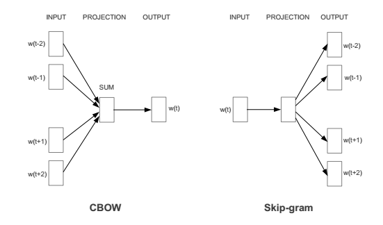
Figure 1: Architecture for the CBOW and Skip-gram method, taken from Efficient Estimation of Word Representations in Vector Space. W(t) is the current word, while w(t-2), w(t-1), etc. are the surrounding words.
These word vectors now capture the context of surrounding words. This can be seen by using basic algebra to find word relations (i.e. “king” – “man” + “woman” = “queen”). These word vectors can be fed into a classification algorithm, as opposed to bag-of-words, to predict sentiment. The advantage is that we now have some word context, and our feature space is much lower (typically ~300 as opposed to ~100,000, which is the size of our vocabulary). We also had to do very little manual feature creation since the neural network was able to extract those features for us. Since text have varying length, one might take the average of all word vectors as the input to a classification algorithm to classify whole text documents.
However, even with the above method of averaging word vectors, we are ignoring word order. As a way to summarize bodies of text of varying length, Quoc Le and Tomas Mikolov came up with the Doc2Vec method. This method is almost identical to Word2Vec, except we now generalize the method by adding a paragraph/document vector. Like Word2Vec, there are two methods: Distributed Memory (DM) and Distributed Bag of Words (DBOW). DM attempts to predict a word given its previous words and a paragraph vector. Even though the context window moves across the text, the paragraph vector does not (hence distributed memory) and allows for some word-order to be captured. DBOW predicts a random group of words in a paragraph given only its paragraph vector (see Figure 2).
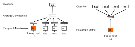
Figure 2: Architecture for Doc2Vec, taken from Distributed Representations of Sentences and Documents.
Once it has been trained, these paragraph vectors can be fed into a sentiment classifier without the need to aggregate words. This method is currently the state-of-the-art when it comes to sentiment classification on the IMDB movie review data set, achieving only a 7.42% error rate. Of course, none of this is useful if we cannot actually implement them. Luckily, a very-well optimized version of Word2Vec and Doc2Vec is available in gensim, a Python library.
Word2Vec Example in Python
In this section we show how one might use word vectors in a sentiment classification task. The gensim library comes standard with the Anaconda distribution or can be installed using pip. From there you can train word vectors on your own corpus (a dataset of text documents) or import pre-trained vectors from C text or binary format:
from gensim.models.word2vec import Word2Vec

model = Word2Vec.load_word2vec_format('vectors.txt', binary=False) #C text format
model = Word2Vec.load_word2vec_format('vectors.bin', binary=True) #C binary format
I find this especially useful when loading Google’s pre-trained word vectors trained over ~100 billion words from the Google News dataset found in the «Pre-trained word and phrase vectors» section here. Note that the file is ~3.5 GB unzipped. Using the Google word vectors we can see some interesting relationships between words:
from gensim.models.word2vec import Word2Vec

model = Word2Vec.load_word2vec_format('GoogleNews-vectors-negative300.bin', binary=True)

model.most_similar(positive=['woman', 'king'], negative=['man'], topn=5)

[(u'queen', 0.711819589138031),
 (u'monarch', 0.618967592716217),
 (u'princess', 0.5902432799339294),
 (u'crown_prince', 0.5499461889266968),
 (u'prince', 0.5377323031425476)]
What’s interesting is that it can find grammatical relationships, for example identifying superlatives or verb stems:
«biggest» — «big» + «small» = «smallest»
model.most_similar(positive=['biggest','small'], negative=['big'], topn=5)

[(u'smallest', 0.6086569428443909),
 (u'largest', 0.6007465720176697),
 (u'tiny', 0.5387299656867981),
 (u'large', 0.456944078207016),
 (u'minuscule', 0.43401968479156494)]
«ate» — «eat» + «speak» = «spoke»
model.most_similar(positive=['ate','speak'], negative=['eat'], topn=5)

[(u'spoke', 0.6965223550796509),
 (u'speaking', 0.6261293292045593),
 (u'conversed', 0.5754593014717102),
 (u'spoken', 0.570488452911377),
 (u'speaks', 0.5630602240562439)]
It’s clear from the above examples that Word2Vec is able to learn non-trivial relationships between words. This is what makes them powerful for many NLP tasks, and in our case sentiment analysis. Before we move on to using them in sentiment analysis, let us first examine Word2Vec’s ability to separate and cluster words. We will use three example word sets: food, sports, and weather words taken from a wonderful website called Enchanted Learning. Since these vectors are 300 dimensional, we will use Scikit-Learn’s implementation of a dimensionality reduction algorithm called t-SNE in order to visualize them in 2D.
First we have to obtain the word vectors as follows:
import numpy as np

with open('food_words.txt', 'r') as infile:
    food_words = infile.readlines()

with open('sports_words.txt', 'r') as infile:
    sports_words = infile.readlines()

with open('weather_words.txt', 'r') as infile:
    weather_words = infile.readlines()

def getWordVecs(words):
    vecs = []
    for word in words:
        word = word.replace('n', '')
        try:
            vecs.append(model[word].reshape((1,300)))
        except KeyError:
            continue
    vecs = np.concatenate(vecs)
    return np.array(vecs, dtype='float') #TSNE expects float type values

food_vecs = getWordVecs(food_words)
sports_vecs = getWordVecs(sports_words)
weather_vecs = getWordVecs(weather_words)
We can then use TSNE and matplotlib to visualize the clusters with the following code:
from sklearn.manifold import TSNE
import matplotlib.pyplot as plt

ts = TSNE(2)
reduced_vecs = ts.fit_transform(np.concatenate((food_vecs, sports_vecs, weather_vecs)))

#color points by word group to see if Word2Vec can separate them
for i in range(len(reduced_vecs)):
    if i < len(food_vecs):
        #food words colored blue
        color = 'b'
    elif i >= len(food_vecs) and i < (len(food_vecs) + len(sports_vecs)):
        #sports words colored red
        color = 'r'
    else:
        #weather words colored green
        color = 'g'
    plt.plot(reduced_vecs[i,0], reduced_vecs[i,1], marker='o', color=color, markersize=8)
The result is as follows:
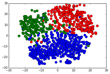
Figure 3: T-SNE projected clusters of food words (blue), sports words (red), and weather words (green).
We can see from the above that Word2Vec does a good job of separating unrelated words, as well as clustering together like words.
Analyzing the Sentiment of Emoji Tweets
Now we will move on to an example in sentiment analysis with tweets gathered using emojis as search terms. We use these emojis as «fuzzy» labels for our data; a smiley emoji (:-)) corresponds to positive sentiment, and a frowny (:-() to negative. The data consists of an even split between positive and negative with a total of ~400,000 tweets. We randomly sample positive and negative tweets to construct an 80/20, train/test, split. We then train the Word2Vec model on the train tweets. In order to prevent data leakage from the test set, we do not train Word2Vec on the test set until after our classifier has been fit on the training set. To construct inputs for our classifier, we take the average of all word vectors in a tweet. We will be using Scikit-Learn to do a lot of the machine learning.
First we import our data and train the Word2Vec model.
from sklearn.cross_validation import train_test_split
from gensim.models.word2vec import Word2Vec

with open('twitter_data/pos_tweets.txt', 'r') as infile:
    pos_tweets = infile.readlines()

with open('twitter_data/neg_tweets.txt', 'r') as infile:
    neg_tweets = infile.readlines()

#use 1 for positive sentiment, 0 for negative
y = np.concatenate((np.ones(len(pos_tweets)), np.zeros(len(neg_tweets))))

x_train, x_test, y_train, y_test = train_test_split(np.concatenate((pos_tweets, neg_tweets)), y, test_size=0.2)

#Do some very minor text preprocessing
def cleanText(corpus):
    corpus = [z.lower().replace('n','').split() for z in corpus]
    return corpus

x_train = cleanText(x_train)
x_test = cleanText(x_test)

n_dim = 300
#Initialize model and build vocab
imdb_w2v = Word2Vec(size=n_dim, min_count=10)
imdb_w2v.build_vocab(x_train)

#Train the model over train_reviews (this may take several minutes)
imdb_w2v.train(x_train)
Next we have to build word vectors for input text in order to average the value of all word vectors in the tweet using the following function:
#Build word vector for training set by using the average value of all word vectors in the tweet, then scale
def buildWordVector(text, size):
    vec = np.zeros(size).reshape((1, size))
    count = 0.
    for word in text:
        try:
            vec += imdb_w2v[word].reshape((1, size))
            count += 1.
        except KeyError:
            continue
    if count != 0:
        vec /= count
    return vec
Scaling moves our data set is part of the process of standardization where we move our dataset into a gaussian distribution with a mean of zero, meaning that values above the mean will be positive, and those below the mean will be negative. Many ML models require scaled datasets to perform effectively, especially those with many features (like text classifiers).
from sklearn.preprocessing import scale
train_vecs = np.concatenate([buildWordVector(z, n_dim) for z in x_train])
train_vecs = scale(train_vecs)

#Train word2vec on test tweets
imdb_w2v.train(x_test)
Finally we have to build our test set vectors and scale them for evaluation.
#Build test tweet vectors then scale
test_vecs = np.concatenate([buildWordVector(z, n_dim) for z in x_test])
test_vecs = scale(test_vecs)
Next we want to validate our classifier by calculating the prediction accuracy on test data, as well as examining its Receiver Operating Characteristic (ROC) curve. ROC curves measure the true-positive rate vs. the false-positive rate of a classifier while adjusting a parameter of the model. In our case, we adjust the cut-off threshold probability for classifying a tweet as positive or negative sentiment. Generally, the larger the Area Under the Curve (AUC), the better our model does at maximizing true positives while minimizing false positives. More on ROC curves can be found here.
To start we’ll train our classifier, in this case using Stochastic Gradient Descent for Logistic Regression.
#Use classification algorithm (i.e. Stochastic Logistic Regression) on training set, then assess model performance on test set
from sklearn.linear_model import SGDClassifier

lr = SGDClassifier(loss='log', penalty='l1')
lr.fit(train_vecs, y_train)

print 'Test Accuracy: %.2f'%lr.score(test_vecs, y_test)
We’ll then create the ROC curve for evaluation using matplotlib and the roc_curve method of Scikit-Learn’s metric package.
#Create ROC curve
from sklearn.metrics import roc_curve, auc
import matplotlib.pyplot as plt

pred_probas = lr.predict_proba(test_vecs)[:,1]

fpr,tpr,_ = roc_curve(y_test, pred_probas)
roc_auc = auc(fpr,tpr)
plt.plot(fpr,tpr,label='area = %.2f' %roc_auc)
plt.plot([0, 1], [0, 1], 'k--')
plt.xlim([0.0, 1.0])
plt.ylim([0.0, 1.05])
plt.legend(loc='lower right')

plt.show()
The resulting curve is as follows:
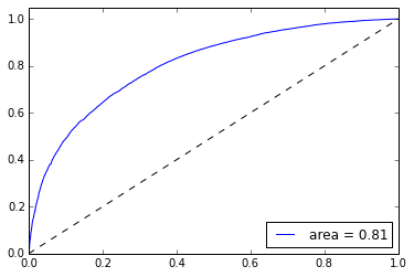
Figure 4: ROC Curve for a logistic classifier on our training data of tweets.
Without any type of feature creation and minimal text preprocessing we can achieve 73% test accuracy using a simple linear model provided by Scikit-Learn. Interestingly, removing punctuation actually causes the accuracy to suffer, suggesting Word2Vec can find interesting features when characters such as «?» and «!» are present. Treating these as individual words, training for longer, doing more preprocessing, and adjusting parameters in both Word2Vec and the classifier could all help in improving accuracy. I have found that using Artificial Neural Networks (ANNs) can improve the accuracy by about 5% when using word vectors. Note that Scikit-Learn does not provide an implementation of ANN classifiers so I used a custom library I created:
from NNet import NeuralNet

nnet = NeuralNet(100, learn_rate=1e-1, penalty=1e-8)
maxiter = 1000
batch = 150
_ = nnet.fit(train_vecs, y_train, fine_tune=False, maxiter=maxiter, SGD=True, batch=batch, rho=0.9)

print 'Test Accuracy: %.2f'%nnet.score(test_vecs, y_test)
The resulting accuracy is 77%. As with any machine learning task, picking the right model is usually more a matter of art than science. If you’d like to use my custom library you can find it on my github. Be warned, it is likely very messy and not regularly maintained! If you would like to contribute please feel free to fork the repository. It could definitely use some TLC!
Using Doc2Vec to Analyze Movie Reviews
Using the averages of word vectors worked fine in the case of tweets. This is because tweets are typically only a few to tens of words in length, which allows us to preserve the relevant features even when averaging. Once we go to the paragraph scale, however, we risk throwing away rich features when we ignore word order and context. In this case it is better to use Doc2Vec to create our input features. As an example we will use the IMDB movie review dataset to test the usefulness of Doc2Vec in sentiment analysis. The data consists of 25,000 positive movie reviews, 25,000 negative, and 50,000 unlabeled reviews. We first train Doc2Vec over the unlabeled reviews. The methodology then identically follows that of the Word2Vec example above, except now we will use both DM and DBOW vectors as inputs by concatenating them.
import gensim

LabeledSentence = gensim.models.doc2vec.LabeledSentence

from sklearn.cross_validation import train_test_split
import numpy as np

with open('IMDB_data/pos.txt','r') as infile:
    pos_reviews = infile.readlines()

with open('IMDB_data/neg.txt','r') as infile:
    neg_reviews = infile.readlines()

with open('IMDB_data/unsup.txt','r') as infile:
    unsup_reviews = infile.readlines()

#use 1 for positive sentiment, 0 for negative
y = np.concatenate((np.ones(len(pos_reviews)), np.zeros(len(neg_reviews))))

x_train, x_test, y_train, y_test = train_test_split(np.concatenate((pos_reviews, neg_reviews)), y, test_size=0.2)

#Do some very minor text preprocessing
def cleanText(corpus):
    punctuation = """.,?!:;(){}[]"""
    corpus = [z.lower().replace('n','') for z in corpus]
    corpus = [z.replace('<br />', ' ') for z in corpus]

    #treat punctuation as individual words
    for c in punctuation:
        corpus = [z.replace(c, ' %s '%c) for z in corpus]
    corpus = [z.split() for z in corpus]
    return corpus

x_train = cleanText(x_train)
x_test = cleanText(x_test)
unsup_reviews = cleanText(unsup_reviews)

#Gensim's Doc2Vec implementation requires each document/paragraph to have a label associated with it.
#We do this by using the LabeledSentence method. The format will be "TRAIN_i" or "TEST_i" where "i" is
#a dummy index of the review.
def labelizeReviews(reviews, label_type):
    labelized = []
    for i,v in enumerate(reviews):
        label = '%s_%s'%(label_type,i)
        labelized.append(LabeledSentence(v, [label]))
    return labelized

x_train = labelizeReviews(x_train, 'TRAIN')
x_test = labelizeReviews(x_test, 'TEST')
unsup_reviews = labelizeReviews(unsup_reviews, 'UNSUP')
These create LabeledSentence type objects:
<gensim.models.doc2vec.LabeledSentence at 0xedd70b70>
Next we instantiate our two Doc2Vec models, DM and DBOW. The gensim documentation suggests training over the data multiple times and either adjusting the learning rate or randomizing the order of input at each pass. We then collect the movie review vectors learned by the models.
import random

size = 400

#instantiate our DM and DBOW models
model_dm = gensim.models.Doc2Vec(min_count=1, window=10, size=size, sample=1e-3, negative=5, workers=3)
model_dbow = gensim.models.Doc2Vec(min_count=1, window=10, size=size, sample=1e-3, negative=5, dm=0, workers=3)

#build vocab over all reviews
model_dm.build_vocab(np.concatenate((x_train, x_test, unsup_reviews)))
model_dbow.build_vocab(np.concatenate((x_train, x_test, unsup_reviews)))

#We pass through the data set multiple times, shuffling the training reviews each time to improve accuracy.
all_train_reviews = np.concatenate((x_train, unsup_reviews))
for epoch in range(10):
    perm = np.random.permutation(all_train_reviews.shape[0])
    model_dm.train(all_train_reviews[perm])
    model_dbow.train(all_train_reviews[perm])

#Get training set vectors from our models
def getVecs(model, corpus, size):
    vecs = [np.array(model[z.labels[0]]).reshape((1, size)) for z in corpus]
    return np.concatenate(vecs)

train_vecs_dm = getVecs(model_dm, x_train, size)
train_vecs_dbow = getVecs(model_dbow, x_train, size)

train_vecs = np.hstack((train_vecs_dm, train_vecs_dbow))

#train over test set
x_test = np.array(x_test)

for epoch in range(10):
    perm = np.random.permutation(x_test.shape[0])
    model_dm.train(x_test[perm])
    model_dbow.train(x_test[perm])

#Construct vectors for test reviews
test_vecs_dm = getVecs(model_dm, x_test, size)
test_vecs_dbow = getVecs(model_dbow, x_test, size)

test_vecs = np.hstack((test_vecs_dm, test_vecs_dbow))
Now we are ready to train a classifier over our review vectors. We will again use sklearn’s SGDClassifier.
from sklearn.linear_model import SGDClassifier

lr = SGDClassifier(loss='log', penalty='l1')
lr.fit(train_vecs, y_train)

print 'Test Accuracy: %.2f'%lr.score(test_vecs, y_test)
This model gives us a test accuracy of 0.86. We can also build a ROC curve for this classifier as follows:
#Create ROC curve
from sklearn.metrics import roc_curve, auc
%matplotlib inline
import matplotlib.pyplot as plt

pred_probas = lr.predict_proba(test_vecs)[:,1]

fpr,tpr,_ = roc_curve(y_test, pred_probas)
roc_auc = auc(fpr,tpr)
plt.plot(fpr,tpr,label='area = %.2f' %roc_auc)
plt.plot([0, 1], [0, 1], 'k--')
plt.xlim([0.0, 1.0])
plt.ylim([0.0, 1.05])
plt.legend(loc='lower right')

plt.show()
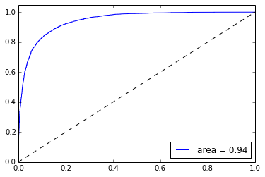
Figure 5: ROC Curve for a logistic classifier on our training data of IMDB movie reviews.
The original paper claimed they saw an improvement when using a 50 node neural network over a simple logistic regression classifier:
from NNet import NeuralNet

nnet = NeuralNet(50, learn_rate=1e-2)
maxiter = 500
batch = 150
_ = nnet.fit(train_vecs, y_train, fine_tune=False, maxiter=maxiter, SGD=True, batch=batch, rho=0.9)

print 'Test Accuracy: %.2f'%nnet.score(test_vecs, y_test)
Interestingly, here we see no such improvement. The test accuracy is 0.85, and we do not approach their claimed test error of 7.42%. This could be for many reasons: we did not train for enough epochs over the training/test data, their implementation of Doc2Vec/ANN is different, their hyperparameters are different, etc. It’s hard to know exactly which since the paper does not go into great detail. In any case, we were able to obtain an 86% test accuracy with very little pre-processing and no feature creation/selection. No fancy convolutions or treebanks necessary!
Conclusion
I hope you have seen not only the utility but ease of use for Word2Vec and Doc2Vec using standard tools like Python and gensim. With a very simple algorithm we can gain rich word and paragraph vectors that can be used in all kinds of NLP applications. What’s even better is Google’s release of their own pre-trained word vectors trained on a much larger data set than anyone else can hope to obtain. If you want to train your own vectors over large data sets there is already an implementation of Word2Vec in Apache Spark’s MLlib. Happy NLP’ing!
Additional Readings
- A Word is Worth a Thousand Vectors
- Word2Vec Tutorial
- Gensim
- Scikit-Learn: Working with Text Data
- Natural Language Processing with Python
If you enjoyed this post and don’t want to miss others like it, click the Subscribe button below.
District Data Labs provides data science consulting and corporate training services. We work with companies and teams of all sizes, helping them make their operations more data-driven and enhancing the analytical abilities of their employees. Interested in working with us? Let us know!
In this article I will describe what is the word2vec algorithm and how one can
use it to implement a sentiment classification system. I will focus essentially on the Skip-Gram model. I won’t explain how to use advanced techniques such as negative sampling. Yet I implemented my sentiment analysis system using negative sampling. My code is available here and it corresponds to the first assignment of the CS224n class from Stanford University about Natural Language Processing with Deep Learning.
The idea behind Word2Vec
There are 2 main categories of Word2Vec methods:
- Continuous Bag of Words Model (or CBOW)
- Skip-Gram Model
While CBOW is a method that tries to “guess” the center word of a sentence knowing its surrounding words, Skip-Gram model tries to determine which words are the most likely to appear next to a center word. In a sense it can be said that these two methods are complementary. For the rest of the article, I will only focus on the Skip-Gram Model.
1. Skip-Gram Model: Intuition
1.1 Training task
Let’s say we want to train our model on one simple sentence like:
«The museums in Paris are amazing»
To do so we will iterate over our sentence and feed our model with a center word and its context words. See
Figure 1.1 for a better understanding.

Figure 1.1: Train a Skip-Gram model using one sentence. The word highlighted in blue is the input word. The word highlighted in red are the context words. Here the window is set to 2, that is to say that we will train our model using 2 words to the left and 2 words to the right of the center word.
1.2 One-Hot representation
Well as we know, we cannot feed a Neural network with words as words have no meaning for a Neural Network (what is the meaning of adding 2 words for example?). We will then transform our words into numbers. One simple idea would be to assign 1 to the first word of our dictionnary, 2 to the next and so on. So for example, assuming we have 40 000 words in our dictionnary:
[a rightarrow 1 \
aardvark rightarrow 2 \
vdots \
zebra rightarrow 40000]
This is a bad idea. Indeed it projects our space of words (40 000 dimensions here) on a line (1 dimension) and loses a lot of information. To better understand why it is not a good idea, imagine dog is the 5641th word of my dictionnary and cat is the 4325th. If we substract cat from dog we have:
5641 (dog) — 4325 (cat) = 1316 (abricot)
We can wonder why substracting cat from dog give us an abricot…
Hence, the naive simplest idea is to assign a vector to each word having a 1 in the position of the word in the vocabulary (dictionnary) and a 0 everywhere else. We call those vectors one-hot vectors.
[a = begin{bmatrix} 1\ 0\ vdots\ 0\ end{bmatrix}
aardvark = begin{bmatrix} 0\ 1\ vdots\ 0\ end{bmatrix}
ldots
zebra = begin{bmatrix} 0\ 0\ vdots\ 1\ end{bmatrix}]
To give you an intuition of why this representation is better, we can use the same example as before. Now, if I substract cat from dog I have a vector with 1 in the 5641th row, -1 in the 4325th row and 0 everywhere else. Therefore we see that this vector could have been obtain using only cat and dog words and not other words. The vector still have information about the word cat and the word dog. Of course this representation isn’t perfect either. These vectors are sparse and they don’t encode any semantic information. That is why we need to transform them into word vectors using a Neural Network.
1.3 Feeding the Neural Network
Now that we have a one-hot vector representing our input word, We will train a 1-hidden layer neural network using these input vectors. The hidden layer has no activation function and we will use a softmax classifier to return the normalized probability of a nearby word appearing next to the center word (input word). The architecture of this Neural network is represented in Figure 1.2:

Figure 1.2: Neural Network Architecture. We usually use between 100 and 1000 hidden features represented by the number of hidden neurons, with 300 being a good default choice.
Note: During the training task, the ouput vector will be one-hot vectors representing the nearby words. On the contray, when we evalute the model the ouput will be a probability distribution (a vector of length 40 000 and whose sum is 1 in our example).
1.4 The Hidden Layer
The idea is to represent a word using another representation then a one-hot vector as one-hot vector prevent us to capture relationship between words (synonyms, belonging, word to adjective,…). So we will represent a word with another vector. To do so we need to represent a word with n number of features (we usually choose n to be between 100 and 1000). The experiments show that 300 features is a good default choice. To have a 300 features word vector we will just need to have 300 neurons in the hidden layer. Hence our weight matrix has shape (300, 40000) and each column of our weight matrix represent a word using 300 features.

Figure 1.3: Weight Matrix. Each column represents a word vector
The idea is to train our model on the task describe in part 1.1. The Neural network will then update our weights and once the task is finished we will only be interested in the weight matrix as it represents each words with features that can capture relationship between words.
What is the effect of the hidden layer? As there is no activation function on the hidden layer when we feed a one-hot vector to the neural network we will multiply the weight matrix by the one hot vector. This will give us the word vector (with 300 features here) corresponding to the input word. See illustration in Figure 1.4 below.

Figure 1.4: Multiplying the weight matrix (in grey) by the one-hot representation of a word will give us the corresponding word vector representation.
1.5 The Ouput Layer
During the ouput layer we multiple a word vector of size (1,300) representing a word in our vocabulary (dictionnary) with the output matrix of size (300,40000). We will then have a (1,40000) ouput vector that we normalize using a softmax classifier to get a probability distribution. For example, with the word aardvark:
[text{input word (40000,1): } aardvark^{intercal} = [0 1 0 ldots 0] \
text{word vector (1,300): } aardvark = [1.2 -3.8 0.17 ldots 0.06] \
text{ouput vector (40000,1): } ouput^{intercal}_{aardvark} = [0.001 0 0.00017 ldots 0.00007]]
This process is also described in Figure 1.5 below:

Figure 1.5: multiplying the output matrix (in grey) by the word vector (in blue) and using softmax classifier we get a (40000,1) vector of probability distribution
1.6 Putting all together
To sum up we use one-hot vector to represent each word of our dictionnary (vocabulary), we then train a simple 1-hidden layer neural network using a center word and its context words. The neural network will update its weight using backpropagation and we will finally retrieve a 300 features vector for each word of our dictionnary. Those 300 features word will be able to encode semantic information.
Actually, if we are feeding two different words that should have a similar context (hot and warm for example), the probability distribution outputed by the neural network for those 2 different words should be quite similar. One way the neural network to ouput similar context predictions is if the word vectors are similar. Hence, if two different words have similar context they are more likely to have a similar word vector representation. This reasoning still apply for words that have similar context but that are not necessary synonyms. For example ski and snowboard should have similar context words and hence similar word vector representation.
2. Skip-Gram Model: Implementation
Now that we gain an intuition on how Skip-Gram model works we will dive into the real subject:
How to implement a Word2Vec model (here Skip-Gram model)?
We saw in part 1 that, for our method to work we need to construct 2 matrices: The weight matrix and the ouput matrix that our neural network will update using backpropagation. As in any Neural Network we can initialize those matrices with small random number. The difficult part resides in finding a good objective function to minimize and compute the gradients to be able to backpropagate the error through the network.
2.1 Notation
We use mathematical notations to encode what we previously saw in part 1:
- Let $m$ be the window size (number of words to the left and to the right of center word)
- Let $n$ be the number of features we choose to encode the word vector ($n = 300$ in part 1)
- Let $v_i$ be the $i^{th}$ word from vocabulary $V$
- Let $|V|$ be the size of the vocabulary $V$ (in our examples from part 1, $|V| = 40000$)
- $W in mathbb{R}^{n times |V|}$ is the input matrix or weight matrix
- $w_i: i^{th}$ column of $W$, the word vector representation of word $v_i$
- $U in mathbb{R}^{|V| times n}$: Ouput word matrix
- $u_i: i^{th}$ row of $U$, the ouput vector representation of word $w_i$
2.2 Steps
We simply rewrite the steps that we saw in part 1 using mathematical notations:
- let $x in mathbb{R}^{|V|}$ be our one-hot input vector of the center word.
- we get the word vector representation: $w_c = Wx in mathbb{R}^n$ (Figure 1.4 from part 1)
- We generate a score vector $z=U w_c$ that we turn into a probability distribution using a
softmax classifier: $widehat{y} = softmax(z)$ (Figure 1.5 from part 1) - We want our probability vector $widehat{y}$ to match the true probability vector which is the sum of
the one-hot representation of the context words that we average over the number of words in our vocabulary to get a probability vector.
2.3 Objective function
To be able to quantify the error between the probabilty vector generated and the true probabilities we need to generate an objective function. Here, we want to maximize the probability of seing the context words knowing the center word. Using math notations we want:
[max J = P(v_{c-m},ldots, v_{c-1}, v_{c+1},ldots, v_{c+m} | v_c)]
Maximizing $J$ is the same as minimizing $-log(J)$ we can rewrite:
[min J = -log[P(v_{c-m},ldots, v_{c-1}, v_{c+1},ldots, v_{c+m} | v_c)]tag{2.1}]
We then use a Naive Bayes assumption. The Naive Bayes assumption states that given the
center word, all context words are independents from each others. In practise this assumption is not true. For example if my center word is snow and my context words are ski and snowboard, it is natural to think that ski are not independant of snowboard given snow in the sense that if ski and snow appears in a text it is more likely that snow will appear than if John and snow appear in a text (John snow doesn’t snowboard…). In practise, using Bayes assumption still gives us good results. We can rewrite (2.1):
[minimize [ -log prodlimits_{j=0, j neq m}^{2m} P(v_{c-m+j} | v_c) ] \
= minimize [ -log prodlimits_{j=0, j neq m}^{2m} P(u_{c-m+j} | w_c) ] \
= minimize [ -log prodlimits_{j=0, j neq m}^{2m} frac{exp(u^{intercal}_{c-m+j} w_c)}{sumlimits_{k=1}^{|V|} exp(u^{intercal}_k w_c)} ] \
= minimize [ — sumlimits_{j=0, j neq m}^{2m} u^{intercal}_{c-m+j} w_c + 2m.log sumlimits_{k=1}^{|V|} exp(u^{intercal}_k w_c)tag{2.2}]
2.4 Implement the Skip-Gram model in Python
Assuming we have already implemented our neural network, we just need to compute the cost function and the gradients with respect to all the other word vectors. Finally we need to update the weights using Stochastic Gradient Descent.
Let:
- target be the index of the center word $v_o$. target (python) = o (in math)
- outputVector be the $U in mathbb{R}^{|V| times n}$: Ouput word matrix
- predicted be $w_c$, the word vector representation of word $v_c$
We implement the cost function using the second to last relation from (2.2) and the previous notations:
[probs = frac{exp(u^{intercal} w_c)}{sumlimits_{k=1}^{|V|} exp(u^{intercal}_k w_c)}]
and then we will retrieve the cost w.r.t to the target word with:
[cost = -log(probs_{o})]
In python we can simply write:
probs = softmax( predicted.dot(outputVectors.T) )
cost = -np.log(probs[target])
This is almost what we want, except that, according to (2.2) we want to compute the cost for $o in [c-m, c+m]${0}. We will do that later, it is quite straightforward. As $log(a times b) = log(a) + log(b)$, we will only need to add up all the costs with $o$ varying betwen $c-m$ and $c+m$.
Now, let’s compute the gradient of $J$ (cost in python) with respect to $w_c$ (predicted in python). We use the chain rule:
[frac{partial J}{partial w_c} = sumlimits_{k=1}^{|V|} frac{partial J}{partial f_k} frac{partial f_k}{partial w_c} \
text{where $f_k = u^{intercal}_k w_c$}]
We already know (see softmax article) that:
[frac{partial J}{partial f_k} = frac{partial }{partial f_k} left( frac{e^{f_o}}{sumlimits_{j=1}^{|V|} e^{f_j}} right) =frac{e^{f_k}}{sumlimits_{j=1}^{|V|} e^{f_j}} — delta_{ko}]
Furthermore:
[frac{partial f_k}{partial w_c} = frac{partial u^{intercal}_k w_c}{partial w_c} =
begin{bmatrix}
frac{d}{d w_{1c}}left(sumlimits_{i=1}^n u_{ki} w_{ic} right)\
frac{d}{d w_{2c}}left(sumlimits_{i=1}^n u_{ki} w_{ic} right)\
vdots \
frac{d}{d w_{nc}}left(sumlimits_{i=1}^n u_{ki} w_{ic} right)\
end{bmatrix}
= u_k]
Finally, using the third point from part 2.2 we can rewrite:
[frac{partial J}{partial w_c} = sumlimits_{k=1}^{|V|}left[frac{e^{f_k}}{sumlimits_{j=1}^{|V|} e^{f_j}} — delta_{ko}right]u_k
= sumlimits_{k=1}^{|V|}(widehat{y}_k — y_k)u_k
= sumlimits_{k=1}^{|V|}(widehat{y} — y)_k
begin{bmatrix}
u_{k1}\
u_{k2}\
vdots \
u_{kn}\
end{bmatrix}
= (widehat{y}-y)U]
To implement this in python, we can write:
# yhat - y
grad_pred = probs
grad_pred[target] -= 1

# dJ/dw_c
grad_pred.dot(outputVectors)
Using the chain rule we can also compute the gradient of $J$ w.r.t all the other word vectors $u$:
[frac{partial J}{partial u_k} = w_c left[frac{e^{f_k}}{sumlimits_{j=1}^{|V|} e^{f_j}} — delta_{ko}right]
= w_c (widehat{y}_k — delta_{ko})]
and in python we can write:
grad = grad_pred[:, np.newaxis] * predicted[np.newaxis, :]
Finally, now that we can compute the cost and the gradients for one nearby word of our input word, we can compute the cost and the gradients for $2m-1$ nearby words of our input word, where $m$ is the size of the window simply by adding up all the costs and all the gradients. Indeed, according to the second to last relation from (2.2), we have:
[log(prodlimits_{k=0, k neq m}^{2m} u_k) = sumlimits_{k=0, k neq m}^{2m} J_k \
text{where $J_k = log(u_k)$}]
As we already computed the gradient and the cost $J_k$ for one $k in [0, 2m]${m} we can retrieve the “final” cost and the “final” gradient simply by adding up all the costs and gradients when $k$ varies between $0$ and $2m$.
In python, supposing we have already implemented a function that computes the cost for one nearby word, we can write something like:
for context_w in contextWords:
    # index of target word
    target = tokens[context_w]

    cost_, gradPred_, gradOut_ = word2vecCostAndGradient(inputVectors[center_w], target, outputVectors, dataset)
    cost += cost_
    gradOut += gradOut_
    gradIn[center_w] += gradPred_

return cost, gradIn, gradOut
3. Sentiment Analysis sytem
3.1 A simple model
A very simple idea to create a sentiment analysis system is to use the average of all the word vectors in a sentence as its features and then try to predict the sentiment level of the said sentence. Here we will use 5 classes to distinguish between very negative sentence (0) and very positive sentence (4).
So we will represent a sentence by taking the average of the vectors of the words in the sentence. In python we can simply write:
# indices of each word of the sentence (indices in [0, |V|])
listOfInd = [tokens[w] for w in sentence]
for i in listOfInd:
    sentVector += wordVectors[i]
sentVector /= len(listOfInd)
We will then just train our neural network using the vector of each sentence as inputs and the classes as desired outputs. Here we use regularization when computing the forward and backward pass to prevent overfitting (generalized poorly on unseen data). Using our system and pretained GloVe vectors we are able to reach 36% accuracy on the dev and test sets (With Word2Vec vectors we are able to reach only 30% accuracy). See Figure 3.1 below.
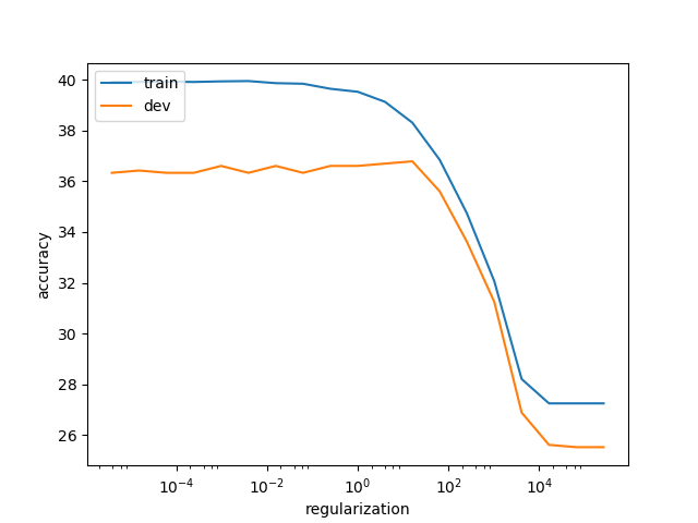
Figure 3.1: Train and dev accuracies for different regularization values using GloVe vectors
Our model clearly overfits when the regularization hyperparameter is less than 10 and we see that both the train and dev accuracies start to decrease when the regularization value is above 10. One good compromise is to choose a regularization parameter around 10 that ensures both a good accuracy and a good generalization on unseen examples.
3.2 Drawback of our model
One big problem of our model is that averaging word vectors to get a representations of our sentences destroys the word order. Hence I can have two sentences with the same words but having different classes (one positive the other negative) and our model will still classify both of them as being the same class. For example:
I like when you don’t know something
I don’t like when you know something
Both sentences have the same words yet the first one seems to be positive while the second one seems to be negative. Our model cannot differentiate between these two sentences and will classify both of them either as being negative or positive. This is a huge drawback.
The fact that we destroy the word order by averaging the word vectors lead to the fact that we cannot recognize the sentiment of complex sentences. For example:
«The best way to hope for any chance of enjoying this film is by lowering your expectation.»
is clearly a negative review. Yet our model will detect the positive words best, hope, enjoy and will say this review is positive. In order to build a better model we will need to keep the order of the words by using a different neural network architecture such as a Recurrent Neural Network.
4. Conclusion
In this article we saw how to train a neural network to transform one-hot vectors into word vectors that have a semantic representation of the words. We also saw how to compute the gradient of the softmax classifier with respect to the word vectors. Finally we implemented a really simple model that can perfom sentiment analysis.
The attentive reader will have noticed that if we have 40,000 words in our vocabulary and if each word is represented by a vector of size 300 then we will need to update 12 million weights at each epoch during training time. It is obviously not what we want to do in practice. It exists other methods like the negative sampling technique or the hierarchical softmax method that allow to reduce the computational cost of training such neural network. Also one thing we need to keep in mind is that if we have 12 million weights to tune we need to have a large dataset of text to prevent overfitting.
Sentiments of words differ from one corpus to another. Inducing general
sentiment lexicons for languages and using them cannot, in general, produce
meaningful results for different domains. In this paper, we combine contextual
and supervised information with the general semantic representations of words
occurring in the dictionary. Contexts of words help us capture the
domain-specific information and supervised scores of words are indicative of
the polarities of those words. When we combine supervised features of words
with the features extracted from their dictionary definitions, we observe an
increase in the success rates. We try out the combinations of contextual,
supervised, and dictionary-based approaches, and generate original vectors. We
also combine the word2vec approach with hand-crafted features. We induce
domain-specific sentimental vectors for two corpora, which are the movie domain
and the Twitter datasets in Turkish. When we thereafter generate document
vectors and employ the support vector machines method utilising those vectors,
our approaches perform better than the baseline studies for Turkish with a
significant margin. We evaluated our models on two English corpora as well and
these also outperformed the word2vec approach. It shows that our approaches are
cross-lingual and cross-domain.
READ FULL TEXT