
Skip to main content
Support
Support
Sign in
Sign in with Microsoft
Sign in or create an account.
Hello,
Select a different account.
You have multiple accounts
Choose the account you want to sign in with.
Quick start
Intro to Excel
Rows & columns
Cells
Formatting
Formulas & functions
Tables
Charts
PivotTables
Share & co-author
Linked data types
Get to know Power Query
 Take a tour
Download template >
 Formula tutorial
Download template >
 Make your first PivotTable
Download template >
 Get more out of PivotTables
Download template >
More resources

Other versions
Excel 2013 training
Other training
LinkedIn Learning Excel training
Templates
Excel templates
Office templates


Need more help?
Want more options?
Discover
Community
Contact Us
Explore subscription benefits, browse training courses, learn how to secure your device, and more.

Microsoft 365 subscription benefits

Microsoft 365 training

Microsoft security

Accessibility center
Communities help you ask and answer questions, give feedback, and hear from experts with rich knowledge.

Ask the Microsoft Community

Microsoft Tech Community

Windows Insiders
Microsoft 365 Insiders
Find solutions to common problems or get help from a support agent.

Online support
Was this information helpful?
(The more you tell us the more we can help.)
(The more you tell us the more we can help.)
What affected your experience?
Resolved my issue
Clear instructions
Easy to follow
No jargon
Pictures helped
Other
Didn’t match my screen
Incorrect instructions
Too technical
Not enough information
Not enough pictures
Other
Any additional feedback? (Optional)
Thank you for your feedback!
×

Learn from live instructors
Microsoft offers live coaching to help your learn excel formulas, tip and more to save you time and to take your skills to the next level.
Get started now
Explore Excel
Find Excel templates
Bring your ideas to life and streamline your work by starting with professionally designed, fully customizable templates from Microsoft Create.
Browse templates

Analyze Data
Ask questions about your data without having to write complicated formulas. Not available in all locales.
Explore your data

Plan and track your health
Tackle your health and fitness goals, stay on track of your progress, and be your best self with help from Excel.
Get healthy

Support for Excel 2013 has ended
Learn what end of Excel 2013 support means for you and find out how you can upgrade to Microsoft 365.
Get the details
Trending topics

In this Microsoft Excel tutorial, we will learn the Microsoft Exel basics. These Microsoft Excel notes will help you learn every MS Excel concepts. Let’s start with the introduction:
What is Microsoft Excel?
Microsoft Excel is a spreadsheet program used to record and analyze numerical and statistical data. Microsoft Excel provides multiple features to perform various operations like calculations, pivot tables, graph tools, macro programming, etc. It is compatible with multiple OS like Windows, macOS, Android and iOS.
A Excel spreadsheet can be understood as a collection of columns and rows that form a table. Alphabetical letters are usually assigned to columns, and numbers are usually assigned to rows. The point where a column and a row meet is called a cell. The address of a cell is given by the letter representing the column and the number representing a row.
Why Should I Learn Microsoft Excel?
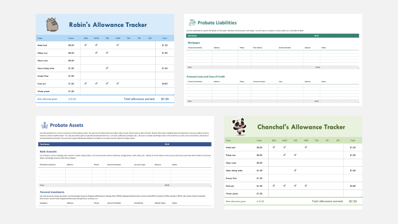
We all deal with numbers in one way or the other. We all have daily expenses which we pay for from the monthly income that we earn. For one to spend wisely, they will need to know their income vs. expenditure. Microsoft Excel comes in handy when we want to record, analyze and store such numeric data. Let’s illustrate this using the following image.

Where can I get Microsoft Excel?
There are number of ways in which you can get Microsoft Excel. You can buy it from a hardware computer shop that also sells software. Microsoft Excel is part of the Microsoft Office suite of programs. Alternatively, you can download it from the Microsoft website but you will have to buy the license key.
In this Microsoft Excel tutorial, we are going to cover the following topics about MS Excel.
- How to Open Microsoft Excel?
- Understanding the Ribbon
- Understanding the worksheet
- Customization Microsoft Excel Environment
- Important Excel shortcuts
How to Open Microsoft Excel?
Running Excel is not different from running any other Windows program. If you are running Windows with a GUI like (Windows XP, Vista, and 7) follow the following steps.
- Click on start menu
- Point to all programs
- Point to Microsoft Excel
- Click on Microsoft Excel
Alternatively, you can also open it from the start menu if it has been added there. You can also open it from the desktop shortcut if you have created one.
For this tutorial, we will be working with Windows 8.1 and Microsoft Excel 2013. Follow the following steps to run Excel on Windows 8.1
- Click on start menu
- Search for Excel N.B. even before you even typing, all programs starting with what you have typed will be listed.
- Click on Microsoft Excel
The following image shows you how to do this

Understanding the Ribbon
The ribbon provides shortcuts to commands in Excel. A command is an action that the user performs. An example of a command is creating a new document, printing a documenting, etc. The image below shows the ribbon used in Excel 2013.

Ribbon components explained
Ribbon start button – it is used to access commands i.e. creating new documents, saving existing work, printing, accessing the options for customizing Excel, etc.
Ribbon tabs – the tabs are used to group similar commands together. The home tab is used for basic commands such as formatting the data to make it more presentable, sorting and finding specific data within the spreadsheet.
Ribbon bar – the bars are used to group similar commands together. As an example, the Alignment ribbon bar is used to group all the commands that are used to align data together.
Understanding the worksheet (Rows and Columns, Sheets, Workbooks)
A worksheet is a collection of rows and columns. When a row and a column meet, they form a cell. Cells are used to record data. Each cell is uniquely identified using a cell address. Columns are usually labelled with letters while rows are usually numbers.
A workbook is a collection of worksheets. By default, a workbook has three cells in Excel. You can delete or add more sheets to suit your requirements. By default, the sheets are named Sheet1, Sheet2 and so on and so forth. You can rename the sheet names to more meaningful names i.e. Daily Expenses, Monthly Budget, etc.

Customization Microsoft Excel Environment
Personally I like the black colour, so my excel theme looks blackish. Your favourite colour could be blue, and you too can make your theme colour look blue-like. If you are not a programmer, you may not want to include ribbon tabs i.e. developer. All this is made possible via customizations. In this sub-section, we are going to look at;
- Customization the ribbon
- Setting the colour theme
- Settings for formulas
- Proofing settings
- Save settings
Customization of ribbon

The above image shows the default ribbon in Excel 2013. Let’s start with customization the ribbon, suppose you do not wish to see some of the tabs on the ribbon, or you would like to add some tabs that are missing such as the developer tab. You can use the options window to achieve this.
- Click on the ribbon start button
- Select options from the drop down menu. You should be able to see an Excel Options dialog window
- Select the customize ribbon option from the left-hand side panel as shown below

- On your right-hand side, remove the check marks from the tabs that you do not wish to see on the ribbon. For this example, we have removed Page Layout, Review, and View tab.
- Click on the “OK” button when you are done.
Your ribbon will look as follows

Adding custom tabs to the ribbon
You can also add your own tab, give it a custom name and assign commands to it. Let’s add a tab to the ribbon with the text Guru99

- Right click on the ribbon and select Customize the Ribbon. The dialogue window shown above will appear
- Click on new tab button as illustrated in the animated image below
- Select the newly created tab
- Click on Rename button
- Give it a name of Guru99
- Select the New Group (Custom) under Guru99 tab as shown in the image below
- Click on Rename button and give it a name of My Commands
- Let’s now add commands to my ribbon bar
- The commands are listed on the middle panel
- Select All chart types command and click on Add button
- Click on OK
Your ribbon will look as follows

Setting the colour theme
To set the color-theme for your Excel sheet you have to go to Excel ribbon, and click on à File àOption command. It will open a window where you have to follow the following steps.

- The general tab on the left-hand panel will be selected by default.
- Look for colour scheme under General options for working with Excel
- Click on the colour scheme drop-down list and select the desired colour
- Click on OK button
Settings for formulas
This option allows you to define how Excel behaves when you are working with formulas. You can use it to set options i.e. autocomplete when entering formulas, change the cell referencing style and use numbers for both columns and rows and other options.

If you want to activate an option, click on its check box. If you want to deactivate an option, remove the mark from the checkbox. You can this option from the Options dialogue window under formulas tab from the left-hand side panel
Proofing settings

This option manipulates the entered text entered into excel. It allows setting options such as the dictionary language that should be used when checking for wrong spellings, suggestions from the dictionary, etc. You can this option from the options dialogue window under the proofing tab from the left-hand side panel
Save settings

This option allows you to define the default file format when saving files, enable auto recovery in case your computer goes off before you could save your work, etc. You can use this option from the Options dialogue window under save tab from the left-hand side panel
Important Excel shortcuts
| Ctrl + P | used to open the print dialogue window |
| Ctrl + N | creates a new workbook |
| Ctrl + S | saves the current workbook |
| Ctrl + C | copy contents of current select |
| Ctrl + V | paste data from the clipboard |
| SHIFT + F3 | displays the function insert dialog window |
| SHIFT + F11 | Creates a new worksheet |
| F2 | Check formula and cell range covered |
Best Practices when working with Microsoft Excel
- Save workbooks with backward compatibility in mind. If you are not using the latest features in higher versions of Excel, you should save your files in 2003 *.xls format for backwards compatibility
- Use description names for columns and worksheets in a workbook
- Avoid working with complex formulas with many variables. Try to break them down into small managed results that you can use to build on
- Use built-in functions whenever you can instead of writing your own formulas
Summary
- Introduction of MS Excel : Microsoft Excel is a powerful spreadsheet program used to record, manipulate, store numeric data and it can be customized to match your preferences
- The ribbon is used to access various commands in Excel
- The options dialogue window allows you to customize a number of items i.e. the ribbon, formulas, proofing, save, etc.
Examples in Each Chapter
We use practical examples to give the user a better understanding of the concepts.
Copy Values Tool
Example values can be copied from the tutorial and into your spreadsheet, making it easy for you to tag along
step-by-step:
Case Based Learning
We have created active learning activities, so you can test and build your knowledge. Making the learning experience more fun and engaging.
Solve Case »
Why Study Excel?
Excel is the world’s most used spreadsheet program.
Example use areas:
- Data analytics
- Project management
- Finance and accounting
Test Yourself With Exercises
My Learning
Track your progress with the free «My Learning» program here at W3Schools.
Log in to your account, and start earning points!
This is an optional feature. You can study W3Schools without using My Learning.

![]()
Download Article
![]()
Download Article
Are you new to Microsoft Excel and need to work on a spreadsheet? Excel is so overrun with useful and complicated features that it might seem impossible for a beginner to learn. But don’t worry—once you learn a few basic tricks, you’ll be entering, manipulating, calculating, and graphing data in no time! This wikiHow tutorial will introduce you to the most important features and functions you’ll need to know when starting out with Excel, from entering and sorting basic data to writing your first formulas.
Things You Should Know
- Use Quick Analysis in Excel to perform quick calculations and create helpful graphs without any prior Excel knowledge.
- Adding your data to a table makes it easy to sort and filter data by your preferred criteria.
- Even if you’re not a math person, you can use basic Excel math functions to add, subtract, find averages and more in seconds.
-

1
Create or open a workbook. When people refer to «Excel files,» they are referring to workbooks, which are files that contain one or more sheets of data on individual tabs. Each tab is called a worksheet or spreadsheet, both of which are used interchangeably. When you open Excel, you’ll be prompted to open or create a workbook.
- To start from scratch, click Blank workbook. Otherwise, you can open an existing workbook or create a new one from one of Excel’s helpful templates, such as those designed for budgeting.
-
2
Explore the worksheet. When you create a new blank workbook, you’ll have a single worksheet called Sheet1 (you’ll see that on the tab at the bottom) that contains a grid for your data. Worksheets are made of individual cells that are organized into columns and rows.
- Columns are vertical and labeled with letters, which appear above each column.
- Rows are horizontal and are labeled by numbers, which you’ll see running along the left side of the worksheet.
- Every cell has an address which contains its column letter and row number. For example, the top-left cell in your worksheet’s address is A1 because it’s in column A, row 1.
- A workbook can have multiple worksheets, all containing different sets of data. Each worksheet in your workbook has a name—you can rename a worksheet by right-clicking its tab and selecting Rename.
- To add another worksheet, just click the + next to the worksheet tab(s).
Advertisement
-
3
Save your workbook. Once you save your workbook once, Excel will automatically save any changes you make by default.[1]
This prevents you from accidentally losing data.- Click the File menu and select Save As.
- Choose a location to save the file, such as on your computer or in OneDrive.
- Type a name for your workbook. All workbooks will automatically inherit the the .XLSX file extension.
- Click Save.


Advertisement
-
1
Click a cell to select it. When you click a cell, it will highlight to indicate that it’s selected.
- When you type something into a cell, the input text is called a value. Entering data into Excel is as simple as typing values into each cell.
- When entering data, the first row of your worksheet (e.g., A1, B1, C1) is typically used as headers for each column. This is helpful when creating graphs or tables which require labels.
- For example, if you’re adding a list of dates in column A, you might click cell A1 and type Date into the cell as the column header.
-
2
Type a word or number into the cell. As you’re typing, you’ll see the letters and/or numbers appear in the cell, as well as in the formula bar at the top of the worksheet.
- When you start practicing more advanced Excel features like creating formulas, this bar will come in handy.
- You can also copy and paste text from other applications into your worksheet, tables from PDFs and the web.
-
3
Press ↵ Enter or ⏎ Return. This enters the data into the cell and moves to the next cell in the column.
-
4
Automatically fill columns based on existing data. Let’s say you want to make a list of consecutive dates or numbers. Or what if you want to fill a column with many of the same values that follow a pattern? As long as Excel can recognize some sort of pattern in your data, such as a particular order, you can use Autofill to automatically populate data into the rest of your column. Here’s a trick to see it in action.
- In a blank column, type 1 into the first cell, 2 into the second cell, and then 3 into the third cell.
- Hover your mouse cursor over the bottom-right corner of the last cell in your series—it will turn to a crosshair.
- Click and drag the crosshair down the column, then release the mouse button once you’ve gone down as far as you like. By default, this will fill the remaining cells with the value of the selected cell—at this point, you’ll probably have something like 1, 2, 3, 3, 3, 3, 3, 3.
- Click the small icon at the bottom-right corner of the filled data to open AutoFill options, and select Fill Series to automatically detect the series or pattern. Now you’ll have a list of consecutive numbers. Try this cool feature out with different patterns!
- Once you get the hang of AutoFill, you’ll have to try flash fill, which you can use to join two columns of data into a single merged column.
-
5
Adjust the column sizes so you can see all of the values. Sometimes typing long values into a cell hides the value and displays hash symbols ### instead of what you’ve typed. If you want to be able to see everything, you can snap the cell contents to the width of the widest cell. For example, let’s say we have some long values in column B:
- To expand the contents of column B, hover the cursor over the dividing line between the B and C at the top of the worksheet—once your cursor is right on the line, it will turn to two arrows pointing in either direction.[2]
- Click and drag the separator until the column is wide enough to accommodate your data, or just double-click the separator to instantly snap the column to the size of the widest value.
- To expand the contents of column B, hover the cursor over the dividing line between the B and C at the top of the worksheet—once your cursor is right on the line, it will turn to two arrows pointing in either direction.[2]
-
6
Wrap text in a cell. If your longer values are now awkwardly long, you can enable text wrapping in one or more cells. Just click a cell (or drag the mouse to select multiple cells), click the Home tab, and then click Wrap Text on the toolbar.
-
7
Edit a cell value. If you need to make a change to a cell, you can double-click the cell to activate the cursor, and then make any changes you need. When you’re finished, just press Enter or Return again.
- To delete the contents of a cell, click the cell once and press delete on your keyboard.
-
8
Apply styles to your data. Whether you want to highlight certain values with color so they stand out or just want to make your data look pretty, changing the colors of cells and their containing values is easy—especially if you’re used to Microsoft Word:
- Select a cell, column, row, or multiple cells at once.
- On the Home tab, click Cell Styles if you’d like to quickly apply quick color styles.
- If you’d rather use more custom options, right-click the selected cell(s) and select Format Cells. Then, use the colors on the Fill tab to customize the cell’s background, or the colors on the Font tab for value colors.
-
9
Apply number formatting to cells containing numbers. If you have data that contains numbers such as prices, measurements, dates, or times, you can apply number formatting to the data so it will display consistently.[3]
By default, the number format is General, which means numbers display exactly as you type them.- Select the cell you want to format. If you’re working with an entire column or row, you can just click the column letter or row number to select the whole thing.
- On the Home tab, click the drop-down menu at the top-center—it’ll say General by default, unless you selected cells that Excel recognizes as a different type of number like Currency or Time.
- Choose one of the formatting options in the list, such as Short Date or Percentage, or click More Number Formats at the bottom to expand all options (we recommend this!).
- If you selected More Number Formats, the Format Cells dialog will expand to the Number tab, where you’ll see several categories for number types.
- Select a category, such as Currency if working with money, or Date if working with dates. Then, choose your preferences, such as a currency symbol and/or decimal places.
- Click OK to apply your formatting.


Advertisement
-
1
Select all of the data you’ve entered so far. Adding your data to a table is the easiest way to work with and analyze data.[4]
Start by highlighting the values you’ve entered so far, including your column headers. Tables also make it easy to sort and filter your data based on values.- Tables traditionally apply different or alternating colors to every other row for easy viewing. Many table options also add borders between cells and/or columns and rows.
-
2
Click Format as Table. You’ll see this at the top-center part of the Home tab.[5]
-
3
Select a table style. Choose any of Excel’s default table styles to get started. You’ll see a small window titled «Create Table» once selected.
- Once you get the hang of tables, you can return here to customize your table further by selecting New Table Style.
-
4
Make sure «My table has headers» is selected and click OK. This tells Excel to turn your column headers into drop-down menus that you can easily sort and filter. Once you click OK, you’ll see that your data now has a color scheme and drop-down menus.
-
5
Click the drop-down menu at the top of a column. Now you’ll see options for sorting that column, as well as several options for filtering all of your data based on its values.
-
6
Choose which data to display based on values in this column. The simplest way to do this is to uncheck the values you don’t want to display—if you uncheck a particular date, for example, you’ll prevent rows that contain the selected date in from appearing in your data. You can also use Text Filters or Number Filters, depending on the type of data in the column:
- If you chose a numerical column, select Number Filters, then choose an option like Greater Than… or Does Not Equal to be extra specific about which values to hide.
- For text columns, you can choose Text Filters, where you can specify things like Begins with or Contains.
- You can also filter by cell color.
-
7
Click OK. Your data is now filtered based on your selections. You’ll also see a small funnel icon in the drop-down menu, which indicates that the data is filtering out certain values.
- To unfilter your data, click the funnel icon, click Clear filter from (column name), and then click OK.
- You can also filter columns that aren’t in tables. Just select a column and click Filter on the Data tab to add a drop-down to that column.
-
8
Sort your data in ascending or descending order. Click the drop-down arrow at the top of a column to view sorting options—these allow you to sort all of your data in order based on the current column.
- If you’re working with numbers, click Smallest to Largest to sort in ascending order, or Largest to Smallest for descending order.[6]
- If you’re working with text values, Sort A to Z will sort in ascending order, while Sort Z to A will sort in reverse.
- When it comes to sorting dates and times, Sort Oldest to Newest will sort with the earliest date at the top and the oldest date at the bottom, and Newest to Oldest displays the dates in descending order.
- When you sort a column, all other columns in the table adjust based on the sort.
- If you’re working with numbers, click Smallest to Largest to sort in ascending order, or Largest to Smallest for descending order.[6]


Advertisement
-
1
Select the data in your worksheet. Excel’s Quick Analysis feature is the easiest way to perform basic calculations (including totals, averages, and counts) and create meaningful tables or graphs without the need for advanced Excel knowledge.[7]
Use your mouse to select your data (including your column headers) to get started. -
2
Click the Quick Analysis icon. This is the small icon that pops up at the bottom-right corner of your selection. It looks like a window with some colored lines.
-
3
Select an analysis type. You’ll see several tabs running along the top of the window, each of which gives you different option for visualizing your data:
- For math calculations, click the Totals tab, where you can select Sum, Average, Count, %Total, or Running Total. You’ll be able to choose whether to display the results at the bottom of each column or to the right.
- To create a chart, click the Charts tab, then select a chart to visualize your data. Before you settle on a chart, just hover the cursor over each option to see a preview.
- To add quick chart data to individual cells, click the Sparklines tab and choose a format. Again, you can hover the cursor over each option to see a preview.
- To instantly apply conditional formatting (which is usually a little more complex in Excel) based on your data, use the Formatting tab. Here you can choose an option like Color or Data Bars, which apply colors to your data based on trends.


Advertisement
-
1
Quickly add data with AutoSum. AutoSum is a built-in Excel function that makes it easy to find the total of one or more columns in a few clicks. Functions or formulas that perform calculations and other tasks based on the values of cells. When you use a function to get something done, you’re creating a formula, which is like a math equation. If you have a column or row of numbers you want to add:
- Click the cell below the numbers you want to add (if a column) or to the right (if a row).[8]
- On the Home tab, click AutoSum toward the upper-right corner of the app. A formula beginning with =SUM(cell+cell) will appear in the field, and a dotted line will surround the numbers you’re adding.
- Press Enter or Return. You should now see the total of the numbers in the selected field. This is here because you created your first formula—which you didn’t have to write by hand!
- If you change any numbers in your data after using AutoSum, the AutoSum value will update automatically.
- Click the cell below the numbers you want to add (if a column) or to the right (if a row).[8]
-
2
Write a simple math formula. AutoSum is just the beginning—Excel is famous for its ability to do all sorts of simple and complex math calculations on data. Fortunately, you don’t have to be a math whiz to create simple formulas to create everyday math formulas, like adding, subtracting, and multiplying. Here’s some basic formulas to get you started:
-
Add: — Type =SUM(cell+cell) (e.g.,
=SUM(A3+B3)) to add two cells’ values together, or type =SUM(cell,cell,cell) (e.g.,=SUM(A2,B2,C2)) to add a series of cell values together.- If you want to add all of the numbers in a whole column (or in a section of a column), type =SUM(cell:cell) (e.g.,
=SUM(A1:A12)) into the cell you want to use to display the result.
- If you want to add all of the numbers in a whole column (or in a section of a column), type =SUM(cell:cell) (e.g.,
-
Subtract: Type =SUM(cell-cell) (e.g.,
=SUM(A3-B3)) to subtract one cell value from another cell’s value. -
Divide: Type =SUM(cell/cell) (e.g.,
=SUM(A6/C5)) to divide one cell’s value by another cell’s value. -
Multiply: Type =SUM(cell*cell) (e.g.,
=SUM(A2*A7)) to multiply two cell values together.
-
Add: — Type =SUM(cell+cell) (e.g.,


Advertisement
-
1
Select a cell for an advanced formula. What if you need to do something more complicated than just adding numbers? Even if you don’t know how to write formulas by hand, you can still create useful formulas that work with your data in various ways. Start by clicking the cell in which you want to display your formula.
-
2
Click the Formulas tab. It’s a tab at the top of the Excel window.
-
3
Explore the Function Library. Several function categories appear in the toolbar, such as Financial, Text, and Math & Trig. Click the options to check out the types of functions available, though they might not make a whole lot of sense just yet.
-
4
Click Insert Function. This option is in the far-left side of the Formulas toolbar. This opens the Insert Function window, which gives you a more detailed breakdown of each function.
-
5
Click a function to learn about it. You can type what you want to do (such as round), or choose a category to filter the list of functions. Then, click any function to read a description of how it works and view its syntax.
- For example, to select the formula for finding the tangent of an angle, you would scroll down and click the TAN option.
-
6
Select a function and click OK. This creates a formula based on the selected function.
-
7
Fill out the function’s formula. When prompted, type in the number or select a cell for which you want to use the formula.
- For example, if you select the TAN function, you’ll type in the number for which you want to find the tangent, or select the cell that contains that number.
- Depending on your selected function, you may need to click through a couple of on-screen prompts.
-
8
Press ↵ Enter or ⏎ Return to run the formula. Doing so applies your function and displays it in your selected cell.


Advertisement
-
1
Set up the chart’s data. If you’re creating a line graph or a bar graph, for example, you’ll want to use one column of cells for the horizontal axis and one column of cells for the vertical axis. The best way to do this is to place your data in a table.
- Typically speaking, the left column is used for the horizontal axis and the column immediately to the right of it represents the vertical axis.
-
2
Select the data in your table. Click and drag your mouse from the top-left cell of the data down to the bottom-right cell of the data.
-
3
Click the Insert tab. It’s a tab at the top of the Excel window.
-
4
Click Recommended Charts. You’ll find this option in the «Charts» section of the Insert toolbar. A window with different chart templates will appear.
-
5
Select a chart template. Click the chart template you want to use based on the type of data you’re working with. If you don’t see a chart type you like, click the All Charts tab to explore by category, such as Pie, Bar, and X Y Scatter.
-
6
Click OK. It’s at the bottom of the window. This creates your chart.
-
7
Use the Chart Design tab to customize your chart. Any time you click your chart, the Chart Design tab will appear at the top of Excel. You can adjust the chart style here, change colors, and add additional elements.
-
8
Double-click a chart element to manage it in the Format panel. When you double-click something on your chart, such as a value, line, or bar, you’ll see options you can edit in the panel on the right side of excel. Here you can change the axis labels, alignment, and legend data.


Advertisement
Add New Question
-
Question
How do you add a check mark or an X mark to a cell?

You can go into Insert, then Symbol, and choose the symbol you want. After that, you can just copy and paste the symbol from one cell to another.
-
Question
Can I add work sheets on Excel?
Yes. At the bottom left of the Excel you will see the list of sheets. To the left of those sheets you will find a «+» sign. Click on it.
-
Question
How do I move cell contents to another cell?
Highlight the cell, right-click, and click Copy. Click destination cell, right-click and Paste.
See more answers
Ask a Question
200 characters left
Include your email address to get a message when this question is answered.
Submit
Advertisement
Video
Thanks for submitting a tip for review!
References
About This Article
Article SummaryX
1. Purchase and install Microsoft Office.
2. Enter data into individual cells.
3. Format cells based on certain criteria.
4. Organize data into rows and columns.
5. Perform math operations using formulas.
6. Use the Formulas tab to find additional formulas.
7. Use data to create charts.
8. Import data from other sources.
Did this summary help you?
Thanks to all authors for creating a page that has been read 646,263 times.
Reader Success Stories
-

«I am applying for a job that requires comprehensive knowledge of Excel. Well, I don’t have it, but this article…» more