Last name from excel

When working with the names dataset in Excel, often there is a need to slice and dice the dataset and extract a part of it.

One common task many Excel users have to do is to extract the last name from the full name.

While it may seem like an easy task, it can get complicated (especially when you’re dealing with data that is not consistent).

In this tutorial, I will show you five different ways to extract the last name from the full name in Excel. I will cover different scenarios, where you only have the first and the last name in the dataset, or the first, middle, and last name.

So let’s get started!

Extract Last Name Using Find and Replace

Extracting the last name from a full name essentially means you’re replacing everything before the last name with a blank.

And this can easily be done using Find and Replace in Excel (and it takes less than 3 seconds).

Below I have a names data set from which I want to extract only the last name.

Below are the steps to use Find and Replace to remove everything before the last name:

1. Copy the name data from Column A and paste it in Column B. I am doing this to keep the original data intact. If you only need the last name, you can skip this step.

1. Select all the names in column B

1. Hold the Control key and press the H key (Command + H if using Mac). This will open the Find and Replace dialog box.

1. In the Find and Replace dialog box, enter the following in the Find what field: * (an asterisk symbol followed by a space character)

1. Leave the Replace with field empty/blank
2. Click on Replace All

The above steps food remove anything before the last space character, which would leave us with the last names only.

The above method would also work in case you have an inconsistent names dataset. For example, if you have names that may or may not have a middle name/initial, or may have a prefix such as Mr or Ms. The only condition is that the last name should be at the end of the name

How does this work?

In the ‘Find what’ field in the Find and Replace dialog box, I have used an asterisk sign (*) followed by a space character.

Asterisk is a wild card character that represents any number of characters in Excel.

So when I ask it to find an asterisk followed by the space character, it will find the last space character in the cell and everything before that space character would be considered a part of the asterisk.

And when I replace it with a blank, everything before the last space character is removed.

Note: For this method to work you need to make sure that there are no trailing spaces in your data. In case there is a space character after the last name, doing the above Find and Replace operation would remove everything from the cell. To make sure there are no trailing spaces, you can use the TRIM formula (read – how to remove trailing spaces in Excel)

Extract Last Name Using Formulas (When you Have Only First and Last name)

Suppose you have a data set as shown below where you have the first name and the last name in column A, and you only want to extract the last name from it.

Below is the formula that will do that:

=RIGHT(A2,LEN(TRIM(A2))-FIND(" ",TRIM(A2)))

Let me quickly explain how this formula works.

The above formula uses the FIND function to get the position of the space character in the name.

Since the position of the space character would be between the first and the last name, once we have the position of the space character, we can use that to extract everything to the right of it (which would be the last name)

But how many characters from the right should it extract?

Since we have the position of the space character, we can subtract that value from the length of the name (which is given by the LEN function). This tells us how many characters are there after the space character in the name.

And this value is then used in the RIGHT formula to extract the last name from the full name.

Note that I have used TRIM(A2) instead of A2 in this formula. This is because there is a possibility that the cells containing the names may have leading, trailing, or double spaces in them. Using the TRIM function makes sure that all these extra spaces are ignored and only one space character between the first name and the last name is considered.

Extract Last Name Using Formulas (When you Have First, Middle, and Last name)

In case you have the first, middle, and last name, the formula becomes a little bit longer.

Below I have a data set where I have the first, middle, last name in column A, and I want to extract the last name from it.

Here is a formula that can do that:

=RIGHT(TRIM(A2),LEN(TRIM(A2))-SEARCH(" ",TRIM(A2),SEARCH(" ",TRIM(A2))+1))

The above function uses the same concept where we have to find out the position of the last space character, and then extract everything to the right of that space character.

But since there are two space characters, in this case, the challenge is to find out the position of this second space character.

To do this, I have used the below-nested SEARCH function (i.e., Search function within a search function)

=SEARCH(" ",TRIM(A2),SEARCH(" ",TRIM(A2))+1)

This part of the formula gives us the position of the second space character, which is then used within the RIGHT formula to extract the last name.

Note that this formula would only work when you have a consistent names dataset – i.e., all the names have the first, middle, and last names.

In case you have a mix of names where some may have middle names but some may not, this formula is not going to work.

If that is the case, use the formula in the next section.

When You Have Incosistent Data (Names with and Without Middle Name)

Below I have a named data set where the format is not consistent – in some cells, we only have the first and last name, and in some cells, there are a middle name and/or prefixes as well.

While you can still use excel formulas to extract the last name in this case, the formula we’ll get a little bit complicated.

Below is the formula that will extract the last name in this inconsistent data set:

=RIGHT(SUBSTITUTE(A2," ","|",LEN(A2)-LEN(SUBSTITUTE(A2," ",""))),LEN(SUBSTITUTE(A2," ","|",LEN(A2)-LEN(SUBSTITUTE(A2," ",""))))-FIND("|",SUBSTITUTE(A2," ","|",LEN(A2)-LEN(SUBSTITUTE(A2," ","")))))

Also read: How to Switch First and Last Name in Excel with Comma?

Extract Last Name using Flash Fill

Another really fast way to extract the last name from full names is by using the Flash Fill feature in Excel.

Introduced in Excel 2013, Flash Fill works by identifying patterns based on user input and giving you the same results for all the cells in the column.

Below I have a data set where I have the names in column A and I want to extract the last name in column B.

Here are the steps to do this Flash Fill:

1. In cell B2, manually enter the last name from the name in cell A2

1. Select the range in column B where you want the last names (B2:B10 in this example)

1. Hold the Control key and press the E key (or Command + E if using Mac)

Note: You can also get the same option when you go to the Home tab, click on the Fill icon, and then click on Flash Fill

The above steps would fill the selected range with the last names from names in Column A.

As I mentioned, Flash Fill works by identifying the pattern in one or two cells where you have manually entered the data and then replicates it for all the other select cells.

In this example, when I entered “Hans” in cell B2, and then used Flash Fill, it recognized that I’m trying to extract the last word from the text string in column A. So we did the same for all the cells I selected.

In case you have a dataset where you have a mix of names with and without a middle name, you can still use Flash Fill to extract the last name.

This is because the pattern that the flash fill has identified is to extract the last word from the text string, so it doesn’t matter how many words are there, it will give you the last name in any case.

Caution: While the flash fill method has worked perfectly in our case, its accuracy is dependent on how well it can identify the pattern. In some cases, it may not be able to identify the right pattern, so it’s important that you double-check the data to make sure it’s correct. In some cases, you may need to enter the data in two or three cells for flash fill to identify the pattern correctly

Compared with the formula method covered above, the flash fill method is a lot faster and more convenient.

One big difference however is that the result of the formula method is dynamic, which means that in case you change the original name, the result in the cell that has the formula would also update.

In the case of Flash Fill, you will have to repeat the same process again to get the updated data

Extract Last Name Using Power Query

If you want to automate the process of extracting the last names from full names, Power Query is the way to go.

For example, if you often have a need to separate names in Excel or to extract the first or last name, you can do that once using Power Query, and the next time you need to do it again, you can simply refresh the query with a single click.

Below I have a data set of names and I want to extract the last name from these. Note that I have a mix of names where there are middle names and prefixes in some of the cells.

Note: When using Power Query, it is best to convert your data into an Excel Table. Doing this would make it a lot easier to work with Power Query, and also allow you to perform the same steps with a single click the next time you add new data set.

To convert your data into an Excel Table, select the data and use the keyboard shortcut Control + T (or Command + T if using Mac)

Below are the steps to use Power Query to get the last name from this dataset:

1. Select any cell in the dataset
2. Click the Data tab in the ribbon

1. In the ‘Get and Transform Data’ group, click on ‘From Selection’. This will open the Power Query editor

1. In the PQ Editor, right-click on the column header

1. Go to the ‘Split Column’ option
2. Click on By Delimiter option.

1. In the ‘Split Column by Delimiter’ dilaog box, select Space as the delimiter (if not selected already)

1. In the Split at options, select ‘Right-most delimiter’

1. Click OK. This will close the dialog box and you will see the result in the PQ Editor

1. Rename the columns the way you want (I am going with ‘Full Name’ and ‘Last Name’)

1. Click on Close and Load option in the ribbon

The above steps would insert a new worksheet in your workbook that would have the resulting table.

Note that in the above example, the first name column has the first name as well as the middle name in some cases. In case you only want the last names, you can delete the first column in Power Query, so it will only give you the last name column as the result in the worksheet.

Now if you’re thinking that this is a long method and you’re better off using Flash Fill or formula method instead, you’re probably right.

The scenario where Power Query really shines is when you get a file that has the data and you need to do multiple modifications to it (say delete some columns, delete blank rows, extract the last name, etc).

The next time you get a new file, you won’t have to repeat all these steps again. simply connect your query to the new file and refresh the query.

In such scenarios, Power Query is a far better solution than using flash fill or formulas or even VBA.

So these are three different methods that you can use to extract the last name from full name in Excel. Personally, I prefer using the Flash Fill method in most cases, as it’s fast and quite reliable.

I hope you found this tutorial useful!

Other Excel tutorials you may also like:

• How to Shuffle a List of Items/Names in Excel?
• How to Combine First and Last Name in Excel)
• How to Sort by the Last Name in Excel
• Extract Usernames from Email Ids in Excel
• Separate First and Last Name in Excel (Split Names Using Formulas)
• How to Extract the First Word from a Text String in Excel

We often need to work with names in Excel. A lot of times we might need to work with a certain part of names in a list.

For example, we might have a list of full names and need to extract the last names to include in a report.

In this tutorial we show you four ways to extract the last name in Excel:

• Using the Text-to-columns feature
• Using the Flash fill feature
• Using a formula
• Using Power Query

Using the Text-to-Columns Feature to Extract the Last Name in Excel

The Text-to-columns feature in Excel lets you separate text in a column into different columns based on a delimiter.

A delimiter is a character or symbol separating text in a cell. For example, in a person’s full name, the delimiter is the space character.

This means you can easily use the Text-to-columns tool to separate names into two different columns – one for the first name and another for the last name.

Once you have the first and last names in separate columns, you can go ahead and delete the column containing the first names, so that you are left with just the last names!

Here’s how you can get this done step-by-step:

Let’s say you have the following list of full names:

To extract the last names for every name in the above list, follow the steps below:

1. Select the list of full names that you want to work with (cell range A2:A7 in our case).
2. Navigate to Data->Data Tools group->Text to Columns.

1. This opens the Convert text to Columns Wizard.
2. At Step 1, check the radio button next to ‘Delimited’.

1. Click Next.
2. At Step 2, uncheck the box next to ‘Tab’ and check the box next to ‘Space’ (since you want to split the names based on the space character).

1. On the right side, there’s a checkbox that says ‘Treat consecutive delimiters as one’. Keep this box checked if there’s a chance your names could have more than one consecutive spaces between them. Checking this option will ensure that Excel trims all the extra space characters.

1. In the preview box at the bottom, you can see how your selected data is going to get split.
2. Click Next.
3. At Step 3, you can specify what format you want your extracted columns to have. Simply leave the default General option selected.

1. In the input field next to ‘Destination’, you need to specify the reference of the cell where you want your separated columns to begin. Since we want to display the separated columns starting from cell B2, we can specify $B$2 in this field.
2. Click Finish.
3. You will now find your names separated into columns B (for first name) and C (for last name).

1. Since you only need the last name, you can go ahead and remove column B. Simply click on the column header, right-click and select ‘Delete’.

You are now left with the last names extracted from your list of names.

Note: This method works if all names contain only first and last names. If any of the names include a middle name, then the method will not work. However, if all the names in the list contained a first, middle, and last name, then you need to follow the same steps. The only difference is that you would then get the list separated into three columns (one for each name) and would need to delete both the first and middle names.

Also read: Remove Middle Name from Full Name in Excel

The Flash fill feature is available in Excel 2013 and later versions.

It’s an intelligent feature that recognizes patterns in your data and automatically fills in columns based on these patterns. 

Here’s how you can use Flash fill to extract the last names from a column of full names:

1. Click on the first cell of your Last Name column (cell B2 in our case).
2. Enter the last name for the first row manually.

1. Click on the Flash fill button from the Data tab. You will find it under the ‘Data Tools’ group. Alternatively you could press the shortcut CTRL+E from your keyboard (Cmd+E if you’re on a Mac).

You should now find the rest of the cells of the Last Name column filled automatically with the last names.

Note: This method also works quite well in recognizing patterns when you have middle names in certain cells. Moreover, it works great in copying patterns, including capitalization and punctuation. So, even if you have your first and last names separated by commas, the flash fill tool does a great job in detecting the pattern and extracting the last names.

Using a Formula to Extract the Last Name in Excel (When you have only First and Last Names)

Now let us look at another way to extract the last name. This time we are going to use a formula.

The formula involves the RIGHT, LEN, and SEARCH functions.

Before looking at the formula, let us first look at what each of these functions does.

The RIGHT Function

The RIGHT function returns a given number of characters from the right side of a given string.

The syntax for this function is as follows:

=RIGHT(text, num_of_characters)

Here,

• text is the input string that you want to work on
• num_of_characters is the number of characters you want to extract from the right side of text.

The LEN Function

This function’s job is simple. It returns the number of characters in a given string.

The syntax for this function is as follows:

=LEN(text)

The function accepts a single parameter, which is the string for which you want to find the number of characters.

The SEARCH Function

The SEARCH function is used to find the location of a given string inside another.

As such, you can use this function to get the location of a space character in a given string too.

The syntax for the SEARCH function is as follows:

=SEARCH (find_text, within_text, [start_num])

Here,

• find_text is the search string that we want to find.
• within_text  is the text that we want search in
• start_num is the position in the text that we want to start searching from. This parameter is optional. If ignored, then it is assumed to be the first position of the text.

Putting Together the RIGHT, LEN and SEARCH Functions to Extract the Last Name

Let us now combine the above three functions into the following formula:

 =RIGHT(A2,LEN(A2)-SEARCH(" ",A2))

Enter the above formula in cell B2 and then copy it down to the rest of the cells. Here’s what we get:

As you can see from the above screenshot, the formula simply extracted the text after the space character in each cell, which is nothing but the last name!

Note: Alternatively, you could use the FIND function instead of the SEARCH function and you would still get the same result.

Explanation of the Formula

Let us break down the above formula to understand how it works.

We are going to go layer by layer, starting from the innermost function:

• SEARCH(“ “,A2)

This finds and returns the position of the space character in the string “Ted Johnson”. It returns the number 4, since the space character is at the 4^th position in the string.

• LEN(A2)-SEARCH(“ “,A2)

This takes the position returned by the SEARCH function and subtracts this from the length of the whole string “Ted Johnson”. This is basically the number of characters in the string after the space character. In other words, it returns the value 11 – 4 = 7.

• RIGHT(A2, LEN(A2)-SEARCH(“ “,A2))

Finally, the RIGHT function extracts LEN(A2)-SEARCH(“ “,A2) characters from the right side of the string.

In this case, it returns the last 7 characters from the string “Ted Johnson”, which simply comprises the last name “Johnson”!

Note: If there’s a chance your names could have more than one consecutive space between them, you can wrap a TRIM function around this formula to trim out the extra spaces: =TRIM(RIGHT(A2, LEN(A2)-SEARCH(“ “,A2)))

Also read: Switch First and Last Name with Comma in Excel (Flip Names)

Formula to Extract the Last Name (When you Have First, Middle and Last Names)

The above formula will only work when you have first and last names on your list.

However, if your list consists of first, middle, and last names, then your formula will be different.

You will then need to slightly tweak the formula to:

=RIGHT(A2,LEN(A2)-SEARCH(" ",A2,SEARCH(" ",A2)+1))

Take a look at a screenshot of how this works with a sample dataset consisting of first, middle, and last names:

Explanation of the Formula

In this case, we used a nested search function to find the location of the last space in the name.

This is because the SEARCH function only returns the location of the first occurrence of the search string.

The inner SEARCH function in our formula returns the location of the first space.

We then used the outer SEARCH function to start looking for the space character, starting its search after the position returned by the inner SEARCH function.

In other words,

• SEARCH(“ “,A2)+1 returns 4, the position of the first space.
• SEARCH(” “,A2,SEARCH(” “,A2)+1) starts searching from the 5th position (4+1) and returns the position of the next space (position 12).
• LEN(A2)-SEARCH(” “,A2,SEARCH(” “,A2)+1) then calculates the number of characters in the last name, which 19 – 12=7.
• And the formula RIGHT(A2,LEN(A2)-SEARCH(” “,A2,SEARCH(” “,A2)+1)) returns the last 7 characters, which is “Johnson”.

In some places, names are specified in reverse, separated by a comma, as follows:

Here, the last name comes before the first name. Moreover, you have a comma separating the names, followed by space.

To extract the last name in such cases, we need to extract the name from the left. So, we need to use the LEFT function.

The LEFT Function

The LEFT function returns a given number of characters from the left side of the string. Syntax of the function is:

LEFT(text, num_of_characters)

Here,

• text is the input string that you want to work on
• num_of_characters is the number of characters you want to extract from the left side of text.

To extract the last name when the names are separated by commas, we use the following formula:

=LEFT(A2,SEARCH(", ",A2)-1)

Let us apply this to our sample list of names:

As you can see from the above screenshot, the formula extracted the text before the comma in each cell, which is basically the last name.

Explanation of the Formula

In the above formula, we simply searched for the comma character in the name, found out its position, and extracted all the characters from the start of the name up to the comma.

Let us break down the formula to understand how it works:

• SEARCH(“, “,A2)

This finds and returns the position of the comma character in the string “Johnson, Ted”. It returns the number 8, since the comma character is at the 8^th position in the string (right after the last name).

• =LEFT(A2,SEARCH(“, “,A2)-1)

This extracts all the characters starting from the left of the string up to one less than the position returned by the SEARCH function. In other words, it returns the first 8 – 1 = 7 characters. This is basically the number of characters in the last name of the string. So the formula returns the last name “Johnson”.

Power Query is a great tool that helps extract and transform data in Excel.

In newer Excel versions, it is available in your Data tab. However, in older versions, you will need to install it as an add-in.

Power Query has a number of amazing data transformation features, which include quickly splitting and/or merging columns. 

Let us see how we can use Power Query to extract the Last Name from a column full names in Excel:

1. Before applying Power Query to your data, you need to convert it to an Excel table. For this, simply select your data and press the shortcut CTRL+T. Alternatively, you could navigate to Insert->Table.

1. This opens the Create Table dialog box. Make sure it shows the correct data range (A1:A7 in our case) and click OK.

1. This will convert your data to an Excel Table.

1. Now you can apply Power Query to your data. Select any cell in the table.
2. From the Data tab, click on the ‘From Table’ button (you will find it under the ‘Get and Transform Data’ group).

1. This opens the Power Query Editor.

1. Right-click on the column header of the Names column and select Split Column->By Delimiter. Alternatively, you could simply click on Split Column->By Delimiter from the Home tab at the top of the Query Editor window.

1. This opens the Split Column by Delimiter dialog box. 

1. Make sure the Space option is selected as the delimiter and the radio button next to ‘Each occurrence of the delimiter’ is checked.
2. Click OK. 
3. Your column should now be split into two parts – one containing the first name and another containing the last name.

1. Double click on the column header for the last name and change the column header name to ‘Last Name’.

1. You can also remove the first column by right-clicking on the column header and selecting ‘Remove’.

1. From the File tab, click on Close & Load.

You should now find a new sheet in your workbook with a table containing your Last Name column. 

Note: If you want to retain the original column containing the full names, then before step 7, select the Add Column tab in the Power Query Editor and select ‘Duplicate Column’. This will create a duplicate of your original column so that you still have the original names in one column while the other one is split into two.

If you’re thinking ‘why bother going through so many steps with the Power Query method, when the other methods are so much simpler’, you have a point.

However, this method is beneficial in the long run, as you can do this once and add it to your power query data cleaning process, so that you don’t have to keep repeating the action for every new worksheet or workbook.

In this tutorial, we showed you four ways to extract the last name in Excel.

We also showed you how to extend these methods to apply them to cases where you have a first, middle, and last name.

We tried to make the tutorial as detailed as we could. So, we hope you found it helpful.

Other articles you may also like:

• How to Extract Text After Space Character in Excel?
• How to Separate Address in Excel?
• How to Add Text to the Beginning or End of all Cells in Excel
• How to Merge First and Last Name in Excel
• How to Remove Commas in Excel (from Numbers or Text String)
• Remove Parentheses (Brackets) in Excel
• How to Remove Dashes (-) in Excel?
• How to Remove a Specific Character from a String in Excel
• How to Find the Last Space in Text String in Excel?
• How to Separate Names in Excel

To extract the first, middle and last name we use the formulas «LEFT», «RIGHT», «MID», «LEN», and «SEARCH» in Excel.

LEFT: Returns the first character(s) in a text string based on the number of characters specified.

Syntax of «LEFT» function: =LEFT (text,[num_chars])

Example:Cell A2 contains the text «Mahesh Kumar Gupta»
=LEFT (A2, 6), function will return «Mahesh»

RIGHT:Return the last character(s) in a text string based on the number of characters specified.

Syntax of «RIGHT» function: =RIGHT (text, [num_chars])

Example:Cell A2 contains the text «Mahesh Kumar Gupta»
=RIGHT (A2, 5), function will return «GUPTA»

MID:Return a specific number of character(s) from a text string, starting at the position specified based on the number of characters specified.

Syntax of «MID» function: =MID (text,start_num,num_chars)

Example:Cell A2 contains the text «Mahesh Kumar Gupta»
=MID (A2, 8, 5), function will return «KUMAR»

LEN:Returns the number of characters in a text string.

Syntax of «LEN» function: =LEN (text)

Example:Cell A2 contains the text «Mahesh Kumar Gupta»
=LEN (A2), function will return 18

SEARCH:The SEARCH function returns the starting position of a text string which it locates from within the text string.

Syntax of «SEARCH» function: =SEARCH (find_text,within_text,[start_num])

Example:Cell A2 contains the text «Mahesh Kumar Gupta»
=SEARCH («Kumar», A2, 1), function will return 8

How to separating the names in Excel through formula? 

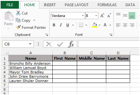
To understand how you can extract the first, middle and last name from the text follow the below mentioned steps:

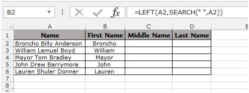
Example 1: We have a list of Names in Column “A” and we need to pick the First name from the list. We will write the «LEFT» function along with the «SEARCH» function.

• Select the Cell B2, write the formula =LEFT (A2, SEARCH (» «, A2)), function will return the first name from the cell A2.
• To Copy the formula in all cells press the key “CTRL + C” and select the cell B3 to B6 and press the key “CTRL + V” on your keyboard.

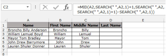
To pick the Middle name from the list. We write the “MID” function along with the “SEARCH” function.

• Select the Cell C2, write the formula =MID(A2,SEARCH(» «,A2,1)+1,SEARCH(» «,A2,SEARCH(» «,A2,1)+1)-SEARCH(» «,A2,1)) it will return the middle name from the cell A2.
• To Copy the formula in all cells press key “CTRL + C” and select the cell C3 to C6 and press key “CTRL + V”on your keyboard.

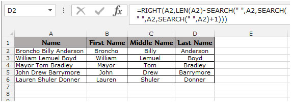
To pick the Last name from the list. We we will use the “RIGHT” function along with the “SEARCH” and “LEN” function.

• Select the Cell D2, write the formula =RIGHT(A2,LEN(A2)-SEARCH(» «,A2,SEARCH(» «,A2,SEARCH(» «,A2)+1))) It will return the last name from the cell A2.
• To Copy the formula in all cells press key “CTRL + C” and select the cell D3 to D6 and press key “CTRL + V” on your keyboard.

This is the way we can split names through formula in Microsoft Excel.

To know more find the below examples:-

Extract file name from a path

How to split a full address into 3 or more separate columns

Learn how to extract last name in Excel in multiple ways with a few simple steps. Note these methods work for extracting other types of data as well (such as first names), but these examples will demonstrate the methods using last names.

Many times data in Excel is not in the necessary format and it takes some cleanup. Fortunately there are a multiple easy ways to clean up data with very little effort.

Extract last name from concatenated first and last name

There are two simple ways to extract the last name from concatenated data within an Excel cell. The first is using a formula to parse the text data and extract the last name. The second is using a build in Excel command called text to columns.

Extract last name using formula

To extract a last name from text data in Excel, a formula using the functions RIGHT, LEN, and SEARCH can be used.

Formula

=RIGHT(text, LEN(text) – SEARCH(” “, text))

Arguments (inputs)

text = the text is the cell containing the concatenated text data of the first and last name

Example

In the example above the RIGHT function selects a defined number of characters from the right hand side of the text in cell B6.

=RIGHT(B6, LEN(B6) – SEARCH(” “, B6))

The number of characters is defined by LEN(B6) – SEARCH(” “, B6). LEN returns the number of characters in the full text, in this case 11 total characters. SEARCH finds the position of the space character (” “), in this case the space is the 7th character. Subtracting the result of SEARCH from the result of LEN provides us with the number of characters in the last name, in this case 4 characters. That value is provided to the RIGHT function, which returns the 4 characters beginning from the right hand side of the text, in this case returning “Gute”.

Extract last name using text to columns

To extract last names from text data using the text to columns command in Excel, follow the steps below:

1. Select the cells you want to extract the last names from
2. Click the Data ribbon –> Text to Columns

1. Leave the Delimited option selected and click Next

1. Check the Space delimiter checkbox and uncheck any other delimiter checkboxes. Click Next.

1. [Optional] Set the destination for the separated data. Click Finish.

In the example above you can see that the last names were extracted from the customer names in column B, and first names placed in column D and last names in column E. We also see that this method had trouble handling a name with multiple spaces (“Darrin Van Huff” in row 8). In this row, the text to column command split the name into three columns with “Huff” in Column F.

Extract last name using Flash Fill

Flash Fill is an a fantastic time saving command that was added in Excel version 2013. Note, it is only available in Excel 2013 and later versions (Excel 2016, 2019, and Excel 365).

1. Type the last name in the cell directly to the right of the first row of the data
2. On the Data tab, click the Flash Fill command (or shortcut Ctrl + E).

The last names will be automatically populated down the column.

Extract name from email address

Names can also be easily extracted from email addresses in Excel. These methods work best when email addresses are formatted in commonly used structures, such as using a period between first and last names or using first initial and last name. For example, john.doe@gmail.com or jdoe@gmail.com.

Extract first and last name using formula

To extract a first and name from an firstname.lastname email address in Excel, a formula using the functions LEFT, MID, and SEARCH can be used.

Formula for extracting first name from email

=LEFT(email, SEARCH(“.”, email) – 1)

Arguments (inputs)

email = the email address, either a cell reference or text string

Example

In the example above the LEFT function selects a defined number of characters from the left hand side of the email in cell B6.

=LEFT(B6, SEARCH(“.”, B6) – 1)

The number of characters is defined by SEARCH(“.”, B6) – 1, which finds the position of the period (.) is with the email address, and subtracts 1. In this case SEARCH(“.”, B6) returns 7. Subtracting 1 returns 6. That value is provided to the LEFT function, which returns the 6 characters beginning from the from the left side of the text, in this case returning the first name “claire”.

Formula for extracting last name from email

=MID(email, SEARCH(“.”, email) + 1, SEARCH(“@”, email) – (SEARCH(“.”, email) + 1))

Arguments (inputs)

email = the email address, either a cell reference or text string

Example

In the example above the MID function selects a defined number of characters from the middle of the email in cell B6.

=MID(B6, SEARCH(“.”, B6) + 1, SEARCH(“@”, B6) – (SEARCH(“.”, B6) + 1))

The position which the MID function begins it’s text extraction is defined by second argument, SEARCH(“.”, B6) + 1, which finds the position of the period (.) is with the email address, and adds 1 because the last name begins after the period. In this case SEARCH(“.”, B6) returns 7, and adding 1 returns 8.

The number of characters returned after that position is defined by the third argument, in this case SEARCH(“@”, B6) – (SEARCH(“.”, B6) + 1). The first SEARCH finds the position of the “@” symbol within the email and subtracts the number of characters from the position of the period (.) + 1. In this case the “@” symbol is character 12, and the period is 7, so the formula returns 12 – (7 +1) = 4.

Those values are provided to the MID function, which returns the 4 characters beginning at character 8, in this case returning the last name “gute”.

Extract name from email using Flash Fill

Flash Fill is an a fantastic time saving command that was added in Excel version 2013. Note, it is only available in Excel 2013 and later versions (Excel 2016, 2019, and Excel 365).

1. Type the names in the cells directly to the right of the first row of the email address data.
2. On the Data tab, click the Flash Fill command (or shortcut Ctrl + E).

The names will be automatically populated down the column, next to the email addresses. If you want first and last names in different columns, you can type the first name and last name in separate cells next to each other and then execute the command and Flash Fill will populate the first and last names in different columns.

EXPLANATION

This tutorial explains how to return only the First name from a name using an Excel formula and VBA.

The Excel method uses a combination of the Excel TRIM, RIGHT, SUBSTITUTE and REPT functions to return the last name from a name.

Both of the VBA methods make use of the Right, Len and InStrRev functions, with the (» «) criteria to return the Last name from a name. The first method shows how the VBA code can be applied if you are only looking to return the Last name from a single cell that captures one name. The second VBA method can be applied if you want to return the Last name from multiple cells that capture one name in each cell, where the VBA code will loop through each cell in the specified range and return the last word from each cell.

FORMULA
=TRIM(RIGHT(SUBSTITUTE(name,» «,REPT(» «,1000)),1000))

ARGUMENTS
name: The name from which you want to retrieve the Last name (Surname).