
Содержание
- LARGE IF & SMALL IF Formulas in Excel & Google Sheets
- LARGE & SMALL Functions
- LARGE IF
- How does the formula work?
- SMALL IF
- LARGE IF with multiple criteria
- IF function – nested formulas and avoiding pitfalls
- Remarks
- Examples
- Additional examples
- Did you know?
- Need more help?
- nth largest value with criteria
- Related functions
- Summary
- Generic formula
- Explanation
- Excel Table
- LARGE function
- LARGE with FILTER
- LARGE with IF
- Multiple criteria
LARGE IF & SMALL IF Formulas in Excel & Google Sheets
Download the example workbook
This tutorial will demonstrate how to calculate “large if” or “small if”, retrieving the nth largest (or smallest) value based on criteria.
LARGE & SMALL Functions
The LARGE Function is used to calculate the nth largest value (k) in an array, while the SMALL Function returns the smallest nth value.
To create a “Large If”, we will use the LARGE Function along with the IF Function in an array formula.
LARGE IF
By combining LARGE (or SMALL) and IF in an array formula, we can essentially create a “LARGE IF” function that works similar to how the built-in SUMIF Function works. Let’s walk through an example.
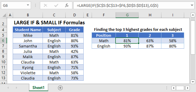
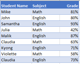
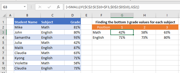
We have a list of grades achieved by students in two different subjects:
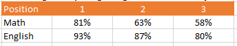
Supposed we are asked to find the top three grades achieved for each subject like so:
To accomplish this, we can nest an IF function with the subject as our criteria inside of the LARGE function like so:
When using Excel 2019 and earlier, you must enter the formula by pressing CTRL + SHIFT + ENTER to get the curly brackets around the formula.
How does the formula work?
The formula works by evaluating each cell in our criteria range as TRUE or FALSE.
Finding the top grade value (k=1) in Math:
Next, the IF Function replaces each value with FALSE if its condition is not met.
Now the LARGE Function skips the FALSE values and calculates the largest (k=1) of the remaining values (0.81 is the largest values between 0.42 and 0.81).
SMALL IF
The same technique can also be applied with the SMALL Function instead.
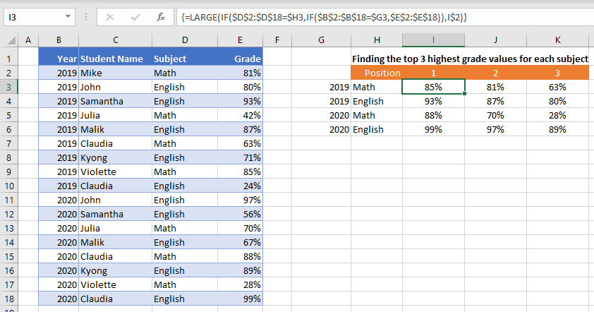
 LARGE IF with multiple criteria
 LARGE IF with multiple criteria
To use LARGE IF with multiple criteria (similar to how the built-in SUMIFS formula works), simply nest more IF functions into the LARGE function like so:
Another way to include multiple criteria is to multiply the criteria together as shown in this article on calculating the Median If.
Источник
IF function – nested formulas and avoiding pitfalls
The IF function allows you to make a logical comparison between a value and what you expect by testing for a condition and returning a result if True or False.
=IF(Something is True, then do something, otherwise do something else)
So an IF statement can have two results. The first result is if your comparison is True, the second if your comparison is False.
IF statements are incredibly robust, and form the basis of many spreadsheet models, but they are also the root cause of many spreadsheet issues. Ideally, an IF statement should apply to minimal conditions, such as Male/Female, Yes/No/Maybe, to name a few, but sometimes you might need to evaluate more complex scenarios that require nesting* more than 3 IF functions together.
* “Nesting” refers to the practice of joining multiple functions together in one formula.
Use the IF function, one of the logical functions, to return one value if a condition is true and another value if it’s false.
IF(logical_test, value_if_true, [value_if_false])
The condition you want to test.
The value that you want returned if the result of logical_test is TRUE.
The value that you want returned if the result of logical_test is FALSE.
While Excel will allow you to nest up to 64 different IF functions, it’s not at all advisable to do so. Why?
Multiple IF statements require a great deal of thought to build correctly and make sure that their logic can calculate correctly through each condition all the way to the end. If you don’t nest your formula 100% accurately, then it might work 75% of the time, but return unexpected results 25% of the time. Unfortunately, the odds of you catching the 25% are slim.
Multiple IF statements can become incredibly difficult to maintain, especially when you come back some time later and try to figure out what you, or worse someone else, was trying to do.
If you find yourself with an IF statement that just seems to keep growing with no end in sight, it’s time to put down the mouse and rethink your strategy.
Let’s look at how to properly create a complex nested IF statement using multiple IFs, and when to recognize that it’s time to use another tool in your Excel arsenal.
Examples
Following is an example of a relatively standard nested IF statement to convert student test scores to their letter grade equivalent.
 97,»A+»,IF(B2>93,»A»,IF(B2>89,»A-«,IF(B2>87,»B+»,IF(B2>83,»B»,IF(B2>79,»B-«,IF(B2>77,»C+»,IF(B2>73,»C»,IF(B2>69,»C-«,IF(B2>57,»D+»,IF(B2>53,»D»,IF(B2>49,»D-«,»F»))))))))))))» loading=»lazy»>
This complex nested IF statement follows a straightforward logic:
If the Test Score (in cell D2) is greater than 89, then the student gets an A
If the Test Score is greater than 79, then the student gets a B
If the Test Score is greater than 69, then the student gets a C
If the Test Score is greater than 59, then the student gets a D
Otherwise the student gets an F
This particular example is relatively safe because it’s not likely that the correlation between test scores and letter grades will change, so it won’t require much maintenance. But here’s a thought – what if you need to segment the grades between A+, A and A- (and so on)? Now your four condition IF statement needs to be rewritten to have 12 conditions! Here’s what your formula would look like now:
It’s still functionally accurate and will work as expected, but it takes a long time to write and longer to test to make sure it does what you want. Another glaring issue is that you’ve had to enter the scores and equivalent letter grades by hand. What are the odds that you’ll accidentally have a typo? Now imagine trying to do this 64 times with more complex conditions! Sure, it’s possible, but do you really want to subject yourself to this kind of effort and probable errors that will be really hard to spot?
Tip: Every function in Excel requires an opening and closing parenthesis (). Excel will try to help you figure out what goes where by coloring different parts of your formula when you’re editing it. For instance, if you were to edit the above formula, as you move the cursor past each of the ending parentheses “)”, its corresponding opening parenthesis will turn the same color. This can be especially useful in complex nested formulas when you’re trying to figure out if you have enough matching parentheses.
Additional examples
Following is a very common example of calculating Sales Commission based on levels of Revenue achievement.
 15000,20%,IF(C9>12500,17.5%,IF(C9>10000,15%,IF(C9>7500,12.5%,IF(C9>5000,10%,0)))))» loading=»lazy»>
This formula says IF(C9 is Greater Than 15,000 then return 20%, IF(C9 is Greater Than 12,500 then return 17.5%, and so on.
While it’s remarkably similar to the earlier Grades example, this formula is a great example of how difficult it can be to maintain large IF statements – what would you need to do if your organization decided to add new compensation levels and possibly even change the existing dollar or percentage values? You’d have a lot of work on your hands!
Tip: You can insert line breaks in the formula bar to make long formulas easier to read. Just press ALT+ENTER before the text you want to wrap to a new line.
Here is an example of the commission scenario with the logic out of order:
 5000,10%,IF(C9>7500,12.5%,IF(C9>10000,15%,IF(C9>12500,17.5%,IF(C9>15000,20%,0)))))» loading=»lazy»>
Can you see what’s wrong? Compare the order of the Revenue comparisons to the previous example. Which way is this one going? That’s right, it’s going from bottom up ($5,000 to $15,000), not the other way around. But why should that be such a big deal? It’s a big deal because the formula can’t pass the first evaluation for any value over $5,000. Let’s say you’ve got $12,500 in revenue – the IF statement will return 10% because it is greater than $5,000, and it will stop there. This can be incredibly problematic because in a lot of situations these types of errors go unnoticed until they’ve had a negative impact. So knowing that there are some serious pitfalls with complex nested IF statements, what can you do? In most cases, you can use the VLOOKUP function instead of building a complex formula with the IF function. Using VLOOKUP, you first need to create a reference table:

This formula says to look for the value in C2 in the range C5:C17. If the value is found, then return the corresponding value from the same row in column D.

Similarly, this formula looks for the value in cell B9 in the range B2:B22. If the value is found, then return the corresponding value from the same row in column C.
Note: Both of these VLOOKUPs use the TRUE argument at the end of the formulas, meaning we want them to look for an approxiate match. In other words, it will match the exact values in the lookup table, as well as any values that fall between them. In this case the lookup tables need to be sorted in Ascending order, from smallest to largest.
VLOOKUP is covered in much more detail here, but this is sure a lot simpler than a 12-level, complex nested IF statement! There are other less obvious benefits as well:
VLOOKUP reference tables are right out in the open and easy to see.
Table values can be easily updated and you never have to touch the formula if your conditions change.
If you don’t want people to see or interfere with your reference table, just put it on another worksheet.
Did you know?
There is now an IFS function that can replace multiple, nested IF statements with a single function. So instead of our initial grades example, which has 4 nested IF functions:
It can be made much simpler with a single IFS function:
The IFS function is great because you don’t need to worry about all of those IF statements and parentheses.
Note: This feature is only available if you have a Microsoft 365 subscription. If you are a Microsoft 365subscriber, make sure you have the latest version of Office.
Need more help?
You can always ask an expert in the Excel Tech Community or get support in the Answers community.
Источник
nth largest value with criteria
Summary
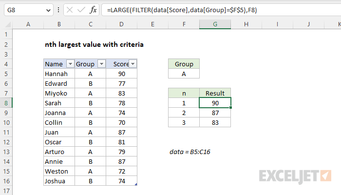
To return the nth largest value that meet specific conditions you can use a formula based on the LARGE function with the FILTER function. In the example shown, the formula in G8 is:
where all data is in an Excel Table called data in the range B5:D16. As the formula is copied down, it returns the top 3 scores in group A, using the value in F5 («A») for group and the value in column F for n.
Note: FILTER is a newer function in Excel. See below for a formula that will work in older versions.
Generic formula
Explanation
In this example, the goal is to retrieve the top 3 scores in column D that appear in a given group, entered as a variable in cell F5. If the group is changed, the formulas should calculate new results. The core of the solution is the LARGE function, which can be used to retrieve the «nth» largest value in a set of data. The challenge is that the LARGE function does not offer any built-in way to apply criteria before calculating a result. This means we need to create our own logic to apply criteria.
There are two basic ways to approach this problem. In the current version of Excel, you can use the FILTER function to apply conditions to data before it is delivered to LARGE. In older versions of Excel, you can use the IF function in an array formula. Both approaches are explained below.
Excel Table
For convenience, all data is in an Excel Table named data in the range B5:D16. Excel Tables are a convenient way to work with data in Excel because they (1) automatically expand to include new data and (2) offer structured references, which let you refer to data by name instead of by address. If you are new to Excel Tables, this article provides an overview. Also see this short video:
LARGE function
The LARGE function is used to return the nth largest value in a set of data like this:
where n is a number like 1, 2, 3, etc. For example, you can retrieve the first, second, and third largest values like this:
The challenge in this problem is that LARGE has no built-in way to apply criteria. One way to apply criteria is with the FILTER function, as described in the next section.
LARGE with FILTER
In the current version of Excel, the FILTER function can be used to apply criteria inside of LARGE. This is the approach used in the worksheet shown, where the formula in G8 is:
Working from the inside out, the FILTER function is configured to extract scores for the group in F5 like this:
Inside FILTER, array is given as the Score column, and the include argument is provided as an expression that compares each value in the Group column to the value in F5 («A»). Note that $F$5 is an absolute reference, because we don’t want this reference to change when the formula is copied down column G. Since there are 12 values in C5:C16, the expression returns an array with 12 TRUE and FALSE values like this:
The TRUE values indicate rows where the group equals «A». This array is used by FILTER to retrieve matching data. The result from FILTER is an array that contains the 6 values in group «A»:
These values are provided to the LARGE function as the array argument. The second argument, k, comes from cell F8:
In cell G8, the result is 90, the (first) largest score in group A. As the formula is copied down, the value for k changes and LARGE returns the second and third best scores in group A.
LARGE with IF
In Legacy Excel, the FILTER function does not exist so we do not have a dedicated function to filter values by group. Instead, we can use a traditional array formula based on the IF function:
Note: this is an array formula and must be entered with control + shift + enter in Legacy Excel.
In this formula, the IF function serves the same purpose as the FILTER function above: it «filters» the values by group. Since we are running a logical test on 12 separate values in the Group column (C5:C16), we get an array that contains 12 results like this:
Notice that only values in group A make it into the array. The values in group B become FALSE when they fail the logical test. This array is returned directly to the LARGE function as the array argument. The value for k comes from cell F8:
LARGE automatically ignores the FALSE values and returns the largest number in the remaining values, which is 90. As the formula is copied down, the value for k changes and LARGE returns the second and third largest values in group A.
Multiple criteria
To apply multiple criteria, you can extend the formula with boolean logic. With FILTER, the generic formula looks like this:
Where criteria1 and criteria2 are expressions to test specific conditions.
In older versions of Excel, you can use the same idea with the IF function like this:
For more information on using Boolean logic in array formulas, see the video below.
Источник
In this example, the goal is to display the top 3 values in C5:C16 that match a specific group, entered as a variable in cell F4. If the group is changed, the formulas should calculate new results. For convenience, group (B5:B16) and value (C5:C16) are named ranges. The core of the solution is the LARGE function, which can be used to retrieve the «nth» largest value in a set of data. The challenge is that the LARGE function does not offer any direct way to apply criteria to the values being processed. This means we need to create our own logic to apply conditions in a separate step.
There are two basic ways to approach this problem. In the current version of Excel, you can use the FILTER function to apply conditions to data before it is delivered to LARGE. In older versions of Excel, you can use the IF function in an array formula. Both approaches are explained below.
LARGE function
The LARGE function can be used to return the nth largest value in a set of data. The generic syntax for LARGE looks like this:
=LARGE(range,n)
where n is a number like 1, 2, 3, etc. For example, you can retrieve the first, second, and third largest values like this:
=LARGE(range,1) // first largest
=LARGE(range,2) // second largest
=LARGE(range,3) // third largest
The challenge in this problem is that LARGE has no built-in way to apply criteria. One way to apply criteria is with the FILTER function, as described in the next section below.
LARGE with FILTER
In the current version of Excel, the FILTER function can be used to apply criteria inside of LARGE. This is the approach used in the worksheet shown, where the formula in F7 is:
=LARGE(FILTER(value,group=$F$4),E7)Working from the inside out, the FILTER function is configured to extract values for the group entered in F4 like this:
=FILTER(value,group=$F$4)Inside FILTER, array is given as value (C5:C16), and the include argument is provided as an expression that compares each value in group (B5:B16) to the value in F4 («A»). Note that $F$4 is an absolute reference, because we don’t want this reference to change when the formula is copied down column F. Since there are 12 values in B5:B16, the expression returns an array that contains 12 TRUE and FALSE values like this:
{TRUE;FALSE;TRUE;FALSE;TRUE;FALSE;TRUE;FALSE;TRUE;FALSE;TRUE;FALSE}The TRUE values indicate rows where the group equals «A». This array is used by FILTER to extract matching values. The result from FILTER is an array that contains the 6 values in the data in group «A»:
{100;70;50;85;91;96}These values are provided to the LARGE function as the array argument. The second argument, k, comes from cell E7:
=LARGE({100;70;50;85;91;96},E7)
=LARGE({100;70;50;85;91;96},1)
=100
As the formula is copied down, the value for k changes and LARGE returns the 1st, 2nd, and 3rd largest numbers in group A.
LARGE with IF
In Legacy Excel, the FILTER function does not exist so we do not have a dedicated function to filter values by group. Instead, we can use a traditional array formula based on the IF function like this:
{=LARGE(IF(group=$F$4,value),E7)}Note: this is an array formula and must be entered with control + shift + enter in Legacy Excel.
In this formula, the IF function provides the same purpose as the FILTER function above: it «filters» the values by group. Since we are running a logical test on a range of cells (B5:B16), we get an array of results. The array returned by IF looks like this:
{100;FALSE;70;FALSE;50;FALSE;85;FALSE;91;FALSE;96;FALSE}Note that only values in group A make it into the array. Group B values become FALSE since they fail the logical test. This array is returned directly to the LARGE function as the array argument. The value for k comes from cell E7:
=LARGE({100;FALSE;70;FALSE;50;FALSE;85;FALSE;91;FALSE;96;FALSE},E7)
=LARGE({100;FALSE;70;FALSE;50;FALSE;85;FALSE;91;FALSE;96;FALSE},1)
=100
LARGE automatically ignores the FALSE values and returns the largest number in the remaining values, which is 100.
Multiple criteria
To take into account multiple criteria, you can extend the formula with boolean logic. With FILTER, the generic formula looks like this:
=LARGE(FILTER(data,(criteria1)*(criteria2),n)
Where criteria1 and criteria2 represent expressions to test specific conditions. In older versions of Excel, you can use the same approach like this:
=LARGE(IF((criteria1)*(criteria2),values),n)
For more information on using Boolean logic in array formulas, see the video below.
You can use the following formulas to perform a LARGE IF function in Excel:
Formula 1: LARGE IF with One Criteria
=LARGE(IF(A2:A16="A",C2:C16),2)
This formula finds the 2nd largest value in C2:C16 where the value in A2:A16 is equal to “A”.
Formula 2: LARGE IF with Multiple Criteria
=LARGE(IF((A2:A16="A")*(B2:B16="Guard"),C2:C16),2)
This formula finds the 2nd largest value in C2:C16 where the value in A2:A16 is equal to “A” and the value in B2:B16 is equal to “Guard”.
The following examples show how to use each formula in practice with the following dataset in Excel:

Example 1: LARGE IF with One Criteria
We can use the following formula to find the 2nd largest value in C2:C16 where the value in A2:A16 is equal to “A”:
=LARGE(IF(A2:A16="A",C2:C16),2)
The following screenshot shows how to use this formula:

This tells us that the 2nd largest points value among all players on team A is 14.
Example 2: LARGE IF with Multiple Criteria
We can use the following formula to find the 2nd largest value in C2:C16 where the value in A2:A16 is equal to “A” and the value in B2:B16 is equal to “Guard”:
=LARGE(IF((A2:A16="A")*(B2:B16="Guard"),C2:C16),2)
The following screenshot shows how to use this formula:

This tells us that the 2nd largest points value among all Guards on team A is 7.
Additional Resources
The following tutorials explain how to perform other common tasks in Excel:
How to Use a Median IF Function in Excel
How to Calculate the Mean and Standard Deviation in Excel
How to Calculate the Interquartile Range (IQR) in Excel
Return to Excel Formulas List
Download Example Workbook
Download the example workbook
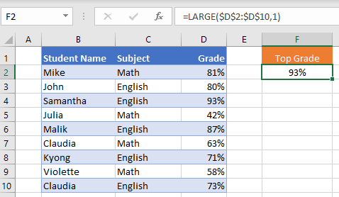
This tutorial will demonstrate how to calculate “large if” or “small if”, retrieving the nth largest (or smallest) value based on criteria.
LARGE & SMALL Functions
The LARGE Function is used to calculate the nth largest value (k) in an array, while the SMALL Function returns the smallest nth value.
=LARGE($D$2:$D$10,1)
To create a “Large If”, we will use the LARGE Function along with the IF Function in an array formula.
LARGE IF
By combining LARGE (or SMALL) and IF in an array formula, we can essentially create a “LARGE IF” function that works similar to how the built-in SUMIF Function works. Let’s walk through an example.
We have a list of grades achieved by students in two different subjects:
Supposed we are asked to find the top three grades achieved for each subject like so:
To accomplish this, we can nest an IF function with the subject as our criteria inside of the LARGE function like so:
=LARGE(IF(<criteria range>=<criteria>, <values range>),<position>)=LARGE(IF($C$2:$C$10=$F3,$D$2:$D$10),G$2)When using Excel 2019 and earlier, you must enter the formula by pressing CTRL + SHIFT + ENTER to get the curly brackets around the formula.
How does the formula work?
The formula works by evaluating each cell in our criteria range as TRUE or FALSE.
Finding the top grade value (k=1) in Math:
=LARGE(IF($C$2:$C$10=$F3,$D$2:$D$10),G$2)=LARGE(IF({TRUE; FALSE;FALSE; TRUE; FALSE; TRUE; FALSE; TRUE; FALSE}, {0.81; 0.8; 0.93; 0.42; 0.87; 0.63; 0.71; 0.58; 0.73}), 1)Next, the IF Function replaces each value with FALSE if its condition is not met.
=LARGE({0.81;FALSE;FALSE;0.42;FALSE;0.63;FALSE;0.58;FALSE},1)Now the LARGE Function skips the FALSE values and calculates the largest (k=1) of the remaining values (0.81 is the largest values between 0.42 and 0.81).
SMALL IF
The same technique can also be applied with the SMALL Function instead.
=SMALL(IF($C$2:$C$10=$F3,$D$2:$D$10),G$2) LARGE IF with multiple criteria
To use LARGE IF with multiple criteria (similar to how the built-in SUMIFS formula works), simply nest more IF functions into the LARGE function like so:
=LARGE(IF(<criteria1 range>=<criteria1>, IF(<criteria2 range>=<criteria2>, <values range>)),<position>)=LARGE(IF($D$2:$D$18=$H3,IF($B$2:$B$18=$G3,$E$2:$E$18)),I$2)
Another way to include multiple criteria is to multiply the criteria together as shown in this article on calculating the Median If.
Tips and tricks:
- Where possible, always reference the position (k) from a helper cell and lock reference (F4) as this will make auto-filling formulas easier.
- If you are using Excel 2019 or newer, you may enter the formula without CTRL + SHIFT + ENTER.
- To retrieve the names of students that achieved the top marks, combine with this with INDEX / MATCH.
Excel for Microsoft 365 Excel for Microsoft 365 for Mac Excel for the web Excel 2021 Excel 2021 for Mac Excel 2019 Excel 2019 for Mac Excel 2016 Excel 2016 for Mac Excel 2013 Excel 2010 Excel 2007 Excel for Mac 2011 Excel Starter 2010 More…Less
This article describes the formula syntax and usage of the LARGE function in Microsoft Excel.
Description
Returns the k-th largest value in a data set. You can use this function to select a value based on its relative standing. For example, you can use LARGE to return the highest, runner-up, or third-place score.
Syntax
LARGE(array, k)
The LARGE function syntax has the following arguments:
-
Array Required. The array or range of data for which you want to determine the k-th largest value.
-
K Required. The position (from the largest) in the array or cell range of data to return.
Remarks
-
If array is empty, LARGE returns the #NUM! error value.
-
If k ≤ 0 or if k is greater than the number of data points, LARGE returns the #NUM! error value.
If n is the number of data points in a range, then LARGE(array,1) returns the largest value, and LARGE(array,n) returns the smallest value.
Example
Copy the example data in the following table, and paste it in cell A1 of a new Excel worksheet. For formulas to show results, select them, press F2, and then press Enter. If you need to, you can adjust the column widths to see all the data.
|
Data |
Data |
|
|---|---|---|
|
3 |
4 |
|
|
5 |
2 |
|
|
3 |
4 |
|
|
5 |
6 |
|
|
4 |
7 |
|
|
Formula |
Description |
Result |
|
=LARGE(A2:B6,3) |
3rd largest number in the numbers above |
5 |
|
=LARGE(A2:B6,7) |
7th largest number in the numbers above |
4 |
Need more help?
Функция НАИБОЛЬШИЙ (LARGE) в Excel используется для получения максимального значения из заданного диапазона ячеек.
Более того, с помощью функции НАИБОЛЬШИЙ в Excel вы сможете задать очередность наибольшего числа по величине. Например из диапазона (1,3,5) вы сможете получить с помощью функции второе по величине число (3).
Содержание
- Что возвращает функция
- Синтаксис
- Аргументы функции
- Дополнительная информация
- Примеры использования функции НАИБОЛЬШИЙ в Excel
- Пример 1. Вычисляем наибольшее число из списка
- Пример 2. Вычисляем второе по величине число из списка
- Пример 3. Использование функции LARGE (НАИБОЛЬШИЙ) с пустыми ячейками
- Пример 4. Использование функции НАИБОЛЬШИЙ с текстовыми значениями
- Пример 5. Использование функции LARGE (НАИБОЛЬШИЙ) в Excel с дублированными данными
- Пример 6. Использование функции НАИБОЛЬШИЙ в Excel с ошибками
Что возвращает функция
Возвращает максимальное значение из заданного диапазона (включая заданную очередность числа по величине).
Синтаксис
=LARGE(array, k) — английская версия
=НАИБОЛЬШИЙ(массив;k) — русская версия
Аргументы функции
- array (массив) — массив или диапазон ячеек из которого вы хотите вычислить максимальное значение;
- k — ранг (очередность числа по величине), которую вам нужно вычислить из диапазона данных.
Дополнительная информация
- если аргумент функции array (массив) пустой, то функция выдаст ошибку;
- если аргумент K ≤ 0 или его значение больше чем количество чисел в диапазоне, то формула выдаст ошибку;
- вы можете указать значение «n» в аргументе k если вы хотите получить последнее (наименьшее) число в диапазоне. Если вы укажете значение «1» в качестве аргумента k то по умолчанию получите максимальное значение из заданного диапазона;
Примеры использования функции НАИБОЛЬШИЙ в Excel
Пример 1. Вычисляем наибольшее число из списка

На примере выше в диапазоне данных A2:A4 у нас есть числа «1»,»8″,»9″. Для того чтобы вычислить наибольшее число из этого диапазона нам поможет формула:
=LARGE(A2:A4,1) — английская версия
=НАИБОЛЬШИЙ(A2:A4;1) — русская версия
Так как аргумент «k» равен «1», функция вернет наибольшее число «9».
Пример 2. Вычисляем второе по величине число из списка
Для того чтобы вычислить второе по величине число из диапазона A2:A4, нам поможет следующая формула:
Больше лайфхаков в нашем Telegram Подписаться
=LARGE(A2:A4,2) — английская версия
=НАИБОЛЬШИЙ(A2:A4;2) — русская версия
Так как значение аргумента «k» мы указали «2», то функция вернет второе по величине значение из диапазона — «8».
Пример 3. Использование функции LARGE (НАИБОЛЬШИЙ) с пустыми ячейками
Если в указанном вами диапазоне данных есть пустые ячейки — функция игнорирует их.
Как показано на примере выше, указав диапазон данных для вычисления «A2:A5″, функция без проблем выдает наибольшее значение «9».
Пример 4. Использование функции НАИБОЛЬШИЙ с текстовыми значениями
Так же как в случае с пустыми ячейками, функция игнорирует текстовые значения, специальные символы, логические выражения.
Пример 5. Использование функции LARGE (НАИБОЛЬШИЙ) в Excel с дублированными данными
В тех случаях, когда в диапазоне данных встречаются два одинаковых значения, функция определит их как последовательные значения. При выводе наибольшего и второго по величине значений, функция выдаст одно и то же значение.
Пример 6. Использование функции НАИБОЛЬШИЙ в Excel с ошибками
В тех случаях, когда в указанном диапазоне есть ячейки с ошибками, функция также выдаст ошибку.
Analyzing data often requires to find the largest value. Sometimes we need to extract the largest value based on a criteria. Excel offers a great solution to find the largest value with criteria. The LARGE and IF functions help us to find the largest value with criteria. In this tutorial, we will learn how to find the largest value with criteria in Excel.
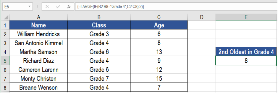 Figure 1. Example of How to Use Large with Criteria in Excel
Generic Formula
{=LARGE(IF(criteria,values),n)}
Here, we use the functions LARGE and IF. LARGE retrieves the “nth” largest value from a numeric data. The IF function here performs a logical test on the range to see if they fulfil the criteria. The values that satisfy the criteria returns those values. The ones that does not satisfy the condition returns FALSE. This array is returned inside the LARGE function. We hardcode the number k for the kth value. This returns the kth largest number.
Setting up Data
The following example uses a student information database. Column A, B and C has the names, ids and ages
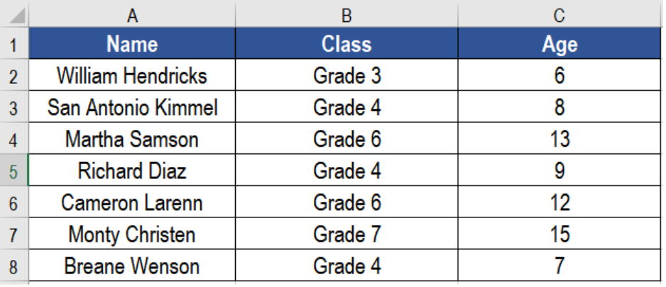 Figure 2. The Sample Data
To find out the second highest age in grade 4, we need to
- Go to cell E5.
- Assign the formula
=LARGE(IF(B2:B8=”Grade 4”,C2:C8),2)to E5. - Press Ctrl + Shift + Enter to apply it as an array formula.
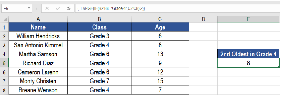 Figure 3. Applying the Formula
This will show the second highest age, which is 8.
Notes
We can find the largest value based on multiple criteria as well. To do that we need to extend the formula based on boolean logic. The formula would have the syntax {=LARGE(IF((criteria 1)*(criteria 2),value),n)}. This will find the nth largest value based on multiple criteria.
Most of the time, the problem you will need to solve will be more complex than a simple application of a formula or function. If you want to save hours of research and frustration, try our live Excelchat service! Our Excel Experts are available 24/7 to answer any Excel question you may have. We guarantee a connection within 30 seconds and a customized solution within 20 minutes.
-
#1
I want to pull the top list on the basis of certain conditions
I am trying to return the top values on the basis of condition, In this case, «I2» should match with Column B
For E.g. if I select, Manufacturing, then it should return the top 20 values from column C wherever in Column B, its Manufacturing
Similarly if I change the filter in cell I2, it should return the top value of that selection only
-
17.4 KB
Views: 5
-
#2
Try…………..
1] Criteria in I1, add heading in I2 and J2
2] In I3 formula, copied across to J3 and all down for 20 rows :
=IFERROR(INDEX($A$1:$C$155,AGGREGATE(15,6,ROW($C$1:$C$155)/($B$1:$B$155=$I$1),ROWS($1:1)),MATCH(I$2,$A$1:$C$1,0)),»»)
Regards
Bosco
-
18.6 KB
Views: 11
-
#3
Perfect Bosco, it was very helpful, it really helped me a lot and made my work a lot easier.
Thank you Once Again
-
#4
B
Try…………..
1] Criteria in I1, add heading in I2 and J2
2] In I3 formula, copied across to J3 and all down for 20 rows :
=IFERROR(INDEX($A$1:$C$155,AGGREGATE(15,6,ROW($C$1:$C$155)/($B$1:$B$155=$I$1),ROWS($1:1)),MATCH(I$2,$A$1:$C$1,0)),»»)
Regards
Bosco
Bosco, Thank you very much for all your help on this.
I was hoping you could also help me in adding more criteria to the list to pull top data
I have added the details in spreadsheet.
-
23.3 KB
Views: 5
-
#5
Hi ,
See if this is OK.
Narayan
-
24.3 KB
Views: 6
-
#6
Thank You Very Narayan, You really are a saviour.
There are couple of more things I was looking at
Is it possible to add a text as «All» in I2 to K2,
The reason I am looking for is:
Score type will be consistent for all:
For e.g: I have selected filer as «Preserving», then it should automatically bring the top score from the entire list of C3 to E156, then as and when I select any other drop down from the list it applies the conditions accordingly.
In other words, If I apply filters on Score Type and Sector as Preserving and Manufacturing respectively, then it should bring the top preserving scores of all the manufacturing accounts, now if select any other drop down either from channel or segment, it should apply consitions accordingly.
-
#7
Hi ,
It can be done , but the formulae will become quite lengthy.
Give me some time.
Narayan
-
#8
Great Narayan,
You can take your time, there is no hurry
-
#9
The attached uses named formulae to break the nested calculation into comprehensible parts. Thus ‘filtered_scores’
= IF(
(Table1[Sector]=Sector) *
(Table1[Channel]=Channel) *
(Table1[Segment]=Segment),
CHOOSE( MATCH( Score_Type, ScoreTypeHeading, 0 ),
Table1[Score1], Table1[Score2], Table1[Score3]) )
and, based upon that, the ‘top_scores’ are
= LARGE(filtered_score,{1;2;3;4;5;6;7;8;9;10})
From there, the companies with the top scores are simply
= INDEX( Table1[Company Name], MATCH( top_scores, filtered_score, 0 ) )
-
29.8 KB
Views: 2
-
#10
As for the rider to you OP, the condition for a match becomes
IF( Sector=»ALL», 1, IF(Table1[Sector]=Sector) )
or, less disruptive in terms of validation, go for blank
IF( Sector=»», 1, IF(Table1[Sector]=Sector) )
-
#11
Thank You Very much Peter for you tremendous help!
The formula to pull the desired list is really very complicated, however I still tried my hand to pull the desired result, but there seems to be some issue with that,
In many cases, it is pulling duplicate values too, my primary moto here is to pull the scores only, because if i have the scores, then i can just use the look up to pull the names.
There are a few things I am not able to understand:
1> Its only pulling 10 scores, however I have tried changing the large function in named range, and tried adding more numbers to it, but its only pulling duplicate names. To look make the list more comprehensive, lets assume that i want to pull all the scores which matches the desired conditions, not just top 10 or top 20 or so.
2> I am not able to understand how to apply the «All» to the drop down, which allows me to pull all the data set
Please provide your thoughts on the same.
-
#12
I have tried changing the large function in named range, and tried adding more numbers to it
This should work provided the punctuation is correct.
In the attached I have replaced the hard-wired sequence with a sequence ‘k’ of length ‘n’ set by the user. This is based upon a helper field containing the record number.
What I implemented was ‘blank’ (simply clear the filter field using Delete)
Because the formula ‘filtered_score’ started to get uncomfortably long, I introduced further Boolean arrays
Sector?: = N( IF(Sector=»», TRUE, Table1[Sector]=Sector) )
Segment?: = N( IF( Segment=»», TRUE, Table1[Segment]=Segment ) )
Channel?: = N( IF( Channel=»», TRUE, Table1[Channel]=Channel ) )
to shorten the final formula. I hope this helps.
-
33.1 KB
Views: 4
-
#13
Thank You Very Narayan, You really are a saviour.
There are couple of more things I was looking at
Is it possible to add a text as «All» in I2 to K2,
The reason I am looking for is:
Score type will be consistent for all:
For e.g: I have selected filer as «Preserving», then it should automatically bring the top score from the entire list of C3 to E156, then as and when I select any other drop down from the list it applies the conditions accordingly.In other words, If I apply filters on Score Type and Sector as Preserving and Manufacturing respectively, then it should bring the top preserving scores of all the manufacturing accounts, now if select any other drop down either from channel or segment, it should apply consitions accordingly.
1] Added «All» to dropdown list of I2,J2 and K2
2] In I4, array formula (Ctrl+Shift+Enter) copied down :
=IFERROR(AGGREGATE(14,6,INDEX($C$3:$E$156,,MATCH($L$2,$C$1:$E$1,0))/IF($I$2=»All»,ISTEXT($B$3:$B$156),$B$3:$B$156=$I$2)/IF($J$2=»All»,ISNUMBER($F$3:$F$156),$F$3:$F$156=$J$2)/IF($K$2=»All»,ISTEXT($G$3:$G$156),$G$3:$G$156=$K$2),ROWS($1:1)),»»)
3] J4, copied down :
=IF(I4=»»,»»,INDEX($A$3:$A$156,MATCH(I4,INDEX($C$3:$E$156,,MATCH($L$2,$C$1:$E$1,0)),0)))
Regards
Bosco
-
23.9 KB
Views: 4
-
#14
Tha
This should work provided the punctuation is correct.
In the attached I have replaced the hard-wired sequence with a sequence ‘k’ of length ‘n’ set by the user. This is based upon a helper field containing the record number.What I implemented was ‘blank’ (simply clear the filter field using Delete)
Because the formula ‘filtered_score’ started to get uncomfortably long, I introduced further Boolean arrays
Sector?: = N( IF(Sector=»», TRUE, Table1[Sector]=Sector) )
Segment?: = N( IF( Segment=»», TRUE, Table1[Segment]=Segment ) )
Channel?: = N( IF( Channel=»», TRUE, Table1[Channel]=Channel ) )to shorten the final formula. I hope this helps.
Thank You Very much Peter, your formula is really amazing, and it is certainly helping me a lot.
However in output column its still only taking 36 entries (column N)
If I enter 154 in cell N8, it should return all of the entries in column N if I have not selected any other drop down.
-
#15
T
1] Added «All» to dropdown list of I2,J2 and K2
2] In I4, array formula (Ctrl+Shift+Enter) copied down :
=IFERROR(AGGREGATE(14,6,INDEX($C$3:$E$156,,MATCH($L$2,$C$1:$E$1,0))/IF($I$2=»All»,ISTEXT($B$3:$B$156),$B$3:$B$156=$I$2)/IF($J$2=»All»,ISNUMBER($F$3:$F$156),$F$3:$F$156=$J$2)/IF($K$2=»All»,ISTEXT($G$3:$G$156),$G$3:$G$156=$K$2),ROWS($1:1)),»»)
3] J4, copied down :
=IF(I4=»»,»»,INDEX($A$3:$A$156,MATCH(I4,INDEX($C$3:$E$156,,MATCH($L$2,$C$1:$E$1,0)),0)))
Regards
Bosco
Thank You very much Bosco, Your formula is great, thank you very very being a saviour.
-
#16
The formula only gave 36 values because it is a multi-cell array formula and had been entered to output the first 36 values from the calculation (This is changed by selecting the entire range you wish to populate and committing the formula using Ctrl+Shift+Enter. Once that has been done the first time it is only necessary to edit the lead cell to change the formula and CSE will populate the entire range)
Note: I would dearly like to reverse the defaults and make the destruction of meaningful arrays involve additional steps
[I looked for the smiley with the horns and evil grin but he seems to have gone missing]
-
36.8 KB
Views: 3
-
#17
1] Added «All» to dropdown list of I2,J2 and K2
2] In I4, array formula (Ctrl+Shift+Enter) copied down :
=IFERROR(AGGREGATE(14,6,INDEX($C$3:$E$156,,MATCH($L$2,$C$1:$E$1,0))/IF($I$2=»All»,ISTEXT($B$3:$B$156),$B$3:$B$156=$I$2)/IF($J$2=»All»,ISNUMBER($F$3:$F$156),$F$3:$F$156=$J$2)/IF($K$2=»All»,ISTEXT($G$3:$G$156),$G$3:$G$156=$K$2),ROWS($1:1)),»»)
3] J4, copied down :
=IF(I4=»»,»»,INDEX($A$3:$A$156,MATCH(I4,INDEX($C$3:$E$156,,MATCH($L$2,$C$1:$E$1,0)),0)))
Regards
Bosco
A bit modified and shorter,
1] I4, array formula copied down :
=IFERROR(AGGREGATE(14,6,INDEX($C$3:$E$156,,MATCH($L$2,$C$1:$E$1,0))/IF($I$2=»All»,1,$B$3:$B$156=$I$2)/IF($J$2=»All»,1,$F$3:$F$156=$J$2)/IF($K$2=»All»,1,$G$3:$G$156=$K$2),ROWS($1:1)),»»)
2] J4, formula copied down :
=IF(I4=»»,»»,INDEX($A$3:$A$156,MATCH(I4,INDEX($C$3:$E$156,,MATCH($L$2,$C$1:$E$1,0)),0)))
Regards
Bosco
-
23.8 KB
Views: 7
-
#18
The formula only gave 36 values because it is a multi-cell array formula and had been entered to output the first 36 values from the calculation (This is changed by selecting the entire range you wish to populate and committing the formula using Ctrl+Shift+Enter. Once that has been done the first time it is only necessary to edit the lead cell to change the formula and CSE will populate the entire range)
Note: I would dearly like to reverse the defaults and make the destruction of meaningful arrays involve additional steps
[I looked for the smiley with the horns and evil grin but he seems to have gone missing]
Thank You Very much Peter, It was great, and it really shows your high spirit towards helping others.
I just wanted to ask one more thing, as you can see that there are only 154 entries in the Table1. so the output are to the maximum limit of 154 only.
I have tried adding more entries to the table, but the same is not reflecting in the output column, I have even tried to reenter the lead formula to reflect the output.
If I am able to solve this one, all of my misery will certainly come to an end.
But all our help is commendable, and I really dont have any more words to thank you enough
-
#19
A bit modified and shorter,
1] I4, array formula copied down :
=IFERROR(AGGREGATE(14,6,INDEX($C$3:$E$156,,MATCH($L$2,$C$1:$E$1,0))/IF($I$2=»All»,1,$B$3:$B$156=$I$2)/IF($J$2=»All»,1,$F$3:$F$156=$J$2)/IF($K$2=»All»,1,$G$3:$G$156=$K$2),ROWS($1:1)),»»)
2] J4, formula copied down :
=IF(I4=»»,»»,INDEX($A$3:$A$156,MATCH(I4,INDEX($C$3:$E$156,,MATCH($L$2,$C$1:$E$1,0)),0)))
Regards
Bosco
Thats great Bosco, thank you very much
-
#20
Thank You Very much Peter, It was great, and it really shows your high spirit towards helping others.
I just wanted to ask one more thing, as you can see that there are only 154 entries in the Table1. so the output are to the maximum limit of 154 only.
I have tried adding more entries to the table, but the same is not reflecting in the output column, I have even tried to reenter the lead formula to reflect the output.
Hi ,
Did you increase the value in Sheet1!$L$8 , from its present value of 154 ?
The output formulae in columns N and O will also need to be edited to include additional rows ; select the entire range N4:N157 , and then extend it to include as many rows as you want , say till row 200 , so that the range N4:N200 is selected ; press F2 and then press CTRL SHIFT ENTER , so that the formula is now entered over the entire range N4:N200.
Do the same for the formula in column O.
The value entered in Sheet1!$L$8 should be less than the number of data rows in the table.
Narayan
-
#21
Hi ,
Did you increase the value in Sheet1!$L$8 , from its present value of 154 ?
The output formulae in columns N and O will also need to be edited to include additional rows ; select the entire range N4:N157 , and then extend it to include as many rows as you want , say till row 200 , so that the range N4:N200 is selected ; press F2 and then press CTRL SHIFT ENTER , so that the formula is now entered over the entire range N4:N200.
Do the same for the formula in column O.
The value entered in Sheet1!$L$8 should be less than the number of data rows in the table.
Narayan
Thank You Narayan, It worked
Thank u very much for all the help
-
#22
@Narayan
Thank you for you support which appears to have established the successful communication of ideas between @msharma864512 and me! I have been out for the day but your intervention probably provided the best solution.
@MSHarma
I hope my way of working was not too unsettling (or even downright baffling) for you. There are other techniques which may be available to you that are more mainstream. For example, if you are going to sort and filter large datasets Power Query might offer an alternative approach. That too, could be something of a culture shock though!
-
#23
@Narayan
Thank you for you support which appears to have established the successful communication of ideas between @msharma864512 and me! I have been out for the day but your intervention probably provided the best solution.@MSHarma
I hope my way of working was not too unsettling (or even downright baffling) for you. There are other techniques which may be available to you that are more mainstream. For example, if you are going to sort and filter large datasets Power Query might offer an alternative approach. That too, could be something of a culture shock though!
Ofcourse not Peter,
I was overwhelmed with seeing so responses from more people like you and it certainly gave me more perspective of solving the complicated things.
-
#24
Thats great Bosco, thank you very much
Hi Bosco,
The formula you created for me was really great,
I am looking for some change in formula.
Is it possible to select multiple entries from a single dropdown to pull the scores. For e.g. in cell I2, I should have the flexibility to select more than one entries at a time, and same is the case with other drop down.
I am looking for something like check box to select multiple entries.
-
23.3 KB
Views: 0