
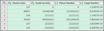
Do you ever import or enter data in Excel that contains leading zeros, like 00123, or large numbers like 1234 5678 9087 6543? Examples of these are social security numbers, phone numbers, credit card numbers, product codes, account numbers, or postal codes. Excel automatically removes leading zeros, and converts large numbers to scientific notation, like 1.23E+15, in order to allow formulas and math operations to work on them. This article deals with how to keep your data in its original format, which Excel treats as text.
Convert numbers to text when you import text data
Use Excel’s Get & Transform (Power Query) experience to format individual columns as text when you import data. In this case, we’re importing a text file, but the data transformation steps are the same for data imported from other sources, such as XML, Web, JSON, etc.
-
Click the Data tab, then From Text/CSV next to the Get Data button. If you don’t see the Get Data button, go to New Query > From File > From Text and browse to your text file, then press Import.
-
Excel will load your data into a preview pane. Press Edit in the preview pane to load the Query Editor.
-
If any columns need to be converted to text, select the column to convert by clicking on the column header, then go to Home > Transform > Data Type > select Text.

Tip: You can select multiple columns with Ctrl+Left-Click.
-
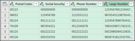
Next, click Replace Current in the Change Column Type dialog, and Excel will convert the selected columns to text.
-
When you’re done, Click Close & Load, and Excel will return the query data to your worksheet.
If your data changes in the future, you can go to Data > Refresh, and Excel will automatically update your data, and apply your transformations for you.
In Excel 2010 and 2013, there are two methods of importing text files and converting numbers to text. The recommended method is to use Power Query, which is available if you download the Power Query add-in. If you can’t download the Power Query add-in, you can use the Text Import Wizard. In this case, we’re importing a text file, but the data transformation steps are the same for data imported from other sources, such as XML, Web, JSON, etc.
-
Click the Power Query tab in the Ribbon, then select Get External Data > From Text.
-
Excel will load your data into a preview pane. Press Edit in the preview pane to load the Query Editor.
-
If any columns need to be converted to text, select the column to convert by clicking on the column header, then go to Home > Transform > Data Type > select Text.
Tip: You can select multiple columns with Ctrl+Left-Click.
-
Next, click Replace Current in the Change Column Type dialog, and Excel will convert the selected columns to text.
-
When you’re done, Click Close & Load, and Excel will return the query data to your worksheet.
If your data changes in the future, you can go to Data > Refresh, and Excel will automatically update your data, and apply your transformations for you.
Use a custom format to keep the leading zeros
If you want to resolve the issue just within the workbook because it’s not used by other programs as a data source, you can use a custom or a special format to keep the leading zeros. This works for number codes that contain fewer than 16 digits. In addition, you can format your number codes with dashes or other punctuation marks. For example, to make a phone number more readable, you can add a dash between the international code, the country/region code, the area code, the prefix, and the last few numbers.
|
Number code |
Example |
Custom number format |
|---|---|---|
|
Social |
012345678 |
000-00-0000 |
|
Phone |
0012345556789 |
00-0-000-000-0000 |
|
Postal |
00123 |
00000 |
Steps
-
Select the cell or range of cells that you want to format.
-
Press Ctrl+1 to load the Format Cells dialog.
-
Select the Number tab, then in the Category list, click Custom and then, in the Type box, type the number format, such as 000-00-0000 for a social security number code, or 00000 for a five-digit postal code.
Tip: You can also click Special, and then select Zip Code, Zip Code + 4, Phone number, or Social Security Number.
Find more information about custom codes, see Create or delete a custom number format.
Note: This will not restore leading zeros that were removed prior to formatting. It will only affect numbers that are entered after the format is applied.
Use the TEXT function to apply a format
You can use an empty column next to your data and use the TEXT function to convert it to the format you want.
|
Number code |
Example (In cell A1) |
TEXT function and new format |
|---|---|---|
|
Social |
012345678 |
=TEXT(A1,»000-00-0000″) |
|
Phone |
0012345556789 |
=TEXT(A1,»00-0-000-000-0000″) |
|
Postal |
00123 |
=TEXT(A1,»00000″) |
Credit card numbers are rounded down
Excel has a maximum precision of 15 significant digits, which means that for any number containing 16 or more digits, such as a credit card number, any numbers past the 15th digit are rounded down to zero. In the case of number codes that are 16 digits or larger, you must use a text format. To do this, you can do one of two things:
-
Format the column as Text
Select your data range and press Ctrl+1 to launch the Format > Cells dialog. On the Number tab, click Text.
Note: This will not change numbers that have already been entered. It will only affect numbers that are entered after the format is applied.
-
Use the apostrophe character
You can type an apostrophe (‘) in front of the number, and Excel will treat it as text.
Top of Page
Need more help?
You can always ask an expert in the Excel Tech Community or get support in the Answers community.
Excel custom number format Millions and Thousands
Many times, you might have large numbers in an Excel report and it is hard to decipher and read the number at one glace.
The best way is to show the numbers in Thousands (K) or Millions (M).
Say, a number 45,200,000 will be displayed as 45.2 Million.

In this article, you will learn about how to do Excel format millions & thousands using:
- Custom Formatting
- With Placeholder Pound Sign (#)
- With Placeholder Zero (0) & Decimal Point
- Round Function
- Conclusion
Let’s get to each point one-by-one.
Custom Formatting
Fortunately, large numbers in Excel can be formatted so they can be shown in “Thousands” or “Millions”.
By using the Format Cells dialogue box shortcuts CTRL+1, you will need to select CUSTOM and then enter one comma to show Thousands or two commas to show Millions. You can even add some text in your cells by entering any word within the quotation marks ” your word “.
But before we move forward, it is important to know that certain characters in custom formatting have specific meaning.
- Zero (0) – Display insignificant zeros
- Pound Sign (#) – Display significant zeros
- Comma (,) – Thousand separator
- Quote (” “) – Add text present within the quotes
You can create Excel Custom Number Format Millions and Thousands using either placeholder zero or pound sign. Let’s look at both of them one-by-one.
With Placeholder Pound Sign (#)
#,##0, “ths”
#,##0,, “mills”
In the example below, you have sales data with the sales amount mentioned in columns D & E. Using the Excel number formatting, you need to convert excel format number in millions & thousands.

Follow the step-by-step tutorial to understand how to add Excel custom number format millions and thousands and make sure to download this workbook to follow along:
DOWNLOAD WORKBOOK
STEP 1: Select Column D in the data below.

STEP 2: Press Ctrl + 1 to open the Format Cells dialog box.

STEP 3: In the Format Cells dialog box, Under Number Tab select Custom.

STEP 4: Type #,##0, “ths” and Click OK.

STEP 5: This is how the Column D after number formatting will look –

STEP 6: Follow the same steps for Column E as well and type #,##0,, “mills” under the custom section.

The only difference between the two customer format (Thousands & Millions) is that you have to put 1 comma for Thousands and two commas for Millions.
Using Placeholder Zero (0) & Decimal Point
0.0, “K”
0.0,, “M”
Zero is used to display insignificant zeros when the number has fewer digits than the format represented using zero. For example, a custom format 0.00 will display number 5, 8.5, and 10.99 as 5.00, 8.50, and 10.99 respectively.
Also, you can round off the number using decimal points symbol.
To get this formatting done, follow the steps below:
STEP 1: Select Column D in the data below.
STEP 2: Right-Click and then Select Format Cells.

STEP 3: In the Format Cells dialog box, Under Number Tab select Custom.
STEP 4: In the Type section, type format – 0.0, “K” and click OK.

Follow the same process for formatting Numbers in Millions.
STEP 4: In the type section, Enter 0.0,, “M” and Click OK.

Excel number format millions & thousands is now ready!

One thing to note is that this will just format the way the number looks like on the Sheet. The number stored in the cell remains the same!
You can use the ROUND function to not just change the formatting but the change the number as well.
ROUND Function
In this method, you have to do three things :
- Divide the number by 1000,000.
- Round off the decimal places.
- Use & sign to add text “M”.
In this example, you have the sales amount mentioned in Column D. Let’s use the combination of division, round, and & sign to get the formatting done.

STEP 1: Select cell E7.

STEP 2: Start with the division. Type =D7/1000000.

STEP 3: Add Round Function to this. Type =ROUND(D7/1000000,1).

STEP 4: Add Text to this formula using & sign. Type =ROUND(D7/1000000,1)&” M”.

STEP 5: Copy the formula down.

STEP 6: Copy the Column and the Press Alt + E + S to open the Paste Special Box and Select Value. Click OK.

The only difference between using Custom Format & Round Function is that :
- In Custom Format, only the formatting changes but the number stored remains the same.

- In Round Function, both the formatting and number changes.

Conclusion
In this article, you have been taught how to do Excel custom number format millions and thousands. There are two ways to do so. You can either use custom format options available in Excel or use a combination of division, round, and & sign.
There are various analytical tools inside Excel, like Conditional Formatting, Data Validation, Tables, Sort & Filter plus MORE! Click here to learn more!
This post is going to show you all the ways you can use to format your large numbers as thousands, millions, or billions.
Large numbers are often used in an Excel spreadsheet, and this can make them difficult to read if they are not formatted properly.
A number in millions or even billions can be difficult to assess and could easily be misread by a factor of 10.
Fortunately, Excel provides several easy ways to format numbers with comma separators to help the user with readability.
If you have ever viewed financial spreadsheets, the numbers are frequently rounded to the nearest thousand because the numbers are often so large. They may even be shown in rounded to the nearest million if the numbers are extremely large.
Not only can displaying numbers as thousands or millions help with readability, but it can also help to fit everything onto a single page.
In this post, I’ll show you 5 easy ways to show your large numbers as thousands or millions. Download the example workbook to follow along!
Use a Simple Formula to Format Numbers as Thousands, Millions, or Billions
An easy way to show numbers in thousands or millions is to use a simple formula to divide the number by a thousand or million.
= B3 / 1000To get a number in the thousand units you can use the above formula.
Cell B3 contains the original number and this formula will calculate the number of thousands, showing the remainder as a decimal number.
= B2 / 1000000To get a number in the million units you can use the above formula. Again this will show anything less than a million as a decimal place.
= B2 / 10 ^ 6One of the problems here might be making sure that you entered the correct number of zeros. This is easy to make a mistake with. A way to get around this is to use the above formula.
The carat character (^) raises the value of 10 to the power of 6, which is 1 million. You can use this same trick when wanting to show values in the billions since 10^9 is equal to 1 billion.
= ROUND ( B3 / 10 ^ 6, 1 )You could also use the ROUND function to remove any excess decimal points from the result. The above formula will result in only one digit after the decimal place.
Note: You will lose the precision in the numbers by using the ROUND function.
Instead, if you want to keep the precision but only show one decimal place you can change the format.
- Select the cells which you want to format.
- Go to the Home tab in the ribbon.
- Click on the decimal format command to decrease the number of decimal places. You may need to click on this a few times depending on how many decimal places you want to show.
Use Paste Special to Format Numbers as Thousands, Millions, or Billions
This is another way to divide your numbers by a thousand or a million, but without using a formula.
You can use a paste special option to divide a number by a thousand or million.
The disadvantage is that it will overwrite the original number, and the process is a bit more complicated. You might want to store the numbers elsewhere in your spreadsheet before using this technique!
- Enter the divisor number such as 1000 into another cell.
- Copy the divisor number (cell D2 in this example) cell by using Ctrl + C or right-clicking on the cell and selecting Copy from the pop-up menu. The cell will have a green dash line around it once it has been copied to the clipboard.
- Select the cells which you want to divide.
- Right-click on the large number to be divided, and select Paste Special from the pop-up menu or press Ctrl + Alt + V on your keyboard.
This will open up the Paste Special menu.
- Select the Divide option found in the Operation section of the Paste Special menu. You may also want to select the Values option under the Paste section so you don’t end up overwriting any formatting you have.
- Press the OK button.
This will overwrite your large numbers with values that have been divided by 1000.
You can use the exact same process to divide your values by a million, a billion, or whatever value is needed.
Use the TEXT Function to Format Numbers as Thousands, Millions, or Billions
The TEXT function in Excel is extremely useful for formatting both numbers and dates to particular formats.
In this case, you can use it to format your numbers as thousands, millions, or billions. The result will be converted to a text value, so this is not an option you’ll want to use if you need to perform any further calculations with the numbers.
Syntax for the TEXT Function
TEXT ( value, format )- value is the numerical value you want to format.
- format is a text string that represents the format rule for the output.
The TEXT function takes a number and will return a text value that’s been formatted.
Example with the TEXT Function
In this post, the TEXT function will be used to add comma separators, hide any thousand digits, and add a k to the end to signify the result is in thousands.
In this example, the large number is in cell B3, and the TEXT formula is used in cell C3.
= TEXT ( B3, "#,##0, " ) & "k"The above formula will show the number from cell B3 as a text value in thousands along with a k to indicate the number is in thousands.
Notice the results are left-aligned? This indicates the results are text values and not numbers.
The hash symbol (#) is used to provide placeholders for the digits of the numbers in the formatting string. The comma symbol (,) is used to provide a divider symbol between the groups of 3 digits.
The zero is included so that should the number be less than 1000, this will show a 0 instead of nothing. If this was just a placeholder (#), then the cell would show nothing instead of a 0 when the number in B3 is less than 1000.
The last comma (,) is needed to indicate that numbers below 1000 will remain hidden as there are no placeholders after this comma.
Note that even when the number in cell B3 is over a million, the placeholders and commas only need to be provided for one group of 3 digits.
The number in cell C3 is far easier to read than the raw number in cell B3.
= TEXT ( B3, "#,##0,, " ) & "M"Use the above formula if you want to display the numbers in millions.
= TEXT ( B3, "#,##0,,, " ) & "B"Use the above formula if you want to display the numbers in billions. An extra comma is all that is needed to hide each set of 3 digits in the results and any character(s) can be added to the end as needed.
Use a Custom Format to Show Numbers as Thousands, Millions, or Billions
It is also possible to format your numbers as thousands or millions using a custom number format.
This way you don’t need to alter the original number or use a formula to show the numbers in your desired format.
You also don’t lose any precision in your numbers as they remain intact and only appear differently.
To add a custom format follow these steps.
- Select the cells for which you want to add custom formatting.
- Press Ctrl + 1 or right click and choose Format Cells to open the Format Cells dialog box.
- Go to the Number tab in the Format Cells menu.
- Select Custom from the Category options.
#,##0, "k"- Add the above format string into the Type field.
- Press the OK button.
#,##0,, "M"If need to show your numbers in millions, use the above format string in step 5 instead.
#,##0,,, "B"If you need to show your numbers in billions, you can use the above format string.
As with the TEXT function, the hash (#) symbols act as placeholders for numbers, and the zero ensures that if the number is zero, a zero will still be displayed rather than a blank.
To display any characters at the end of your numbers, you will need to insert them between two double-quote characters.
Below the Type field, you will notice there is a large set of predefined custom formats. You can select any of these and modify them in the same way as the above thousand or millions formats.
This can be an easy way to create a thousand or million format that also allows for negative numbers.
#,##0,, "M";[Red](#,##0,,) "M"For example, the above will format numbers in millions but also show negative numbers in red with surrounding parentheses.
Any new formats you create will be listed along with all the other predefined custom formats and you can use the Delete button to remove any of the custom formats you have created.
The best thing about using a custom format is you can still do further calculations on the formatted numbers. The original numbers remain unchanged. It’s only the appearance of the numbers that have changed.
Use Conditional Formatting to Format Numbers as Thousands, Millions, or Billions
Can also format numbers according to their value. This can be done by creating a conditional formatting rule for a cell or a range of cells such that the following happens.
- Shows the number as normal if less than 1k
- Shows the number as thousands when between 1k and 1M
- Shows the number as millions when over 1M
Follow these steps to create this conditional format.
- Select the cell or range of cells that you wish to format.
- Go to the Home tab in the ribbon.
- Click on the Conditional Formatting command found in the Styles group.
- Select New Rule from the options.
- Select the Format only cells that contain option found under the Select a Rule Type list.
- Under the Format only cells with settings, select Cell Value and greater than or equal to in the dropdown menus then enter 1000 into the input box.
- Click on the Format button to choose what formatting will show when the conditions are met.
This will open a lighter version of the Format Cells menu with only a Number, Font, Border, and Fill tab.
- Go to the Number tab.
- Select Custom from the Category options available.
#,##0, "k"- Enter the above string into the Type section. If you’ve already used this custom formatting elsewhere, you’ll also be able to select it from the predefined options below the Type field.
- Press the Ok button.
This will close the Format Cells menu and the New Formatting Rule menu will be back in focus. Now you should see a preview of the formatting which will be applied when the formula is true.
- Press the OK button to close the New Formatting Rule menu and save your new conditional formatting rule.
Now you will see any numbers in your selection appear normal when they are less than 1000 and appear in thousands when they are above 1000.
Now you repeat the above steps to add another conditional formatting rule to take care of numbers that are over 1000000.
The process is the exact same as before with slight changes to the Format only cells with input and the Custom format used.
In step 6 enter the value 1000000 into the input box.
#,##0,, "M"In step 10 use the above custom format.
Now you will see your numbers appear with a mix of formatting depending on the value. Numbers under 1k appear normal, while numbers over 1k but under 1M are shown in thousands, and numbers over 1M are shown in millions.
For numbers less than 1k the default general format is adequate since there is no need for comma separators.
If you are expecting negative numbers, you will need to repeat the process to add rules for numbers less than or equal to -1000 and less than or equal to -1000000.
Conclusions
There are many ways in Excel to present large numbers to the user.
These all make the numbers easier to read and prevent mistakes from being made when someone is reading a number off of a report.
If the report is large in width, it may be very necessary to show the numbers in thousands, millions, or even billions so that they can fit on the page.
Using custom formatting of numbers and also conditional formatting, there are many ways to highlight specific values of numbers to draw them to the attention of the user.
Do you use any of these tips for showing large numbers in thousands, millions, or billions? Do you know any other methods? Let me know in the comments below!
About the Author
John is a Microsoft MVP and qualified actuary with over 15 years of experience. He has worked in a variety of industries, including insurance, ad tech, and most recently Power Platform consulting. He is a keen problem solver and has a passion for using technology to make businesses more efficient.
I will show you how to display large, even huge, numbers in Excel. In Excel, you can’t show numbers that are too big but, there is a way around this.
The reason Excel can’t store and display really large numbers is because it is not an inherently mathematical program; it’s not meant for really complex mathematical equations that require exceptionally accurate calculations.
The Problem
Display the following number in Excel:
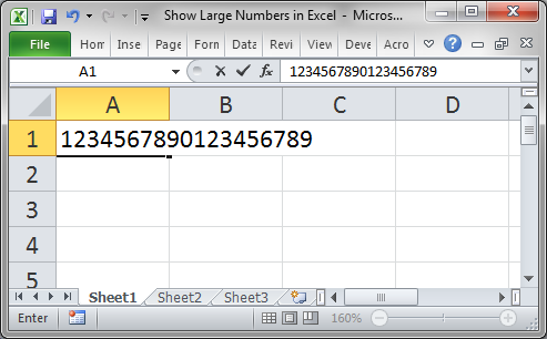
When we hit Enter, this is what we get:
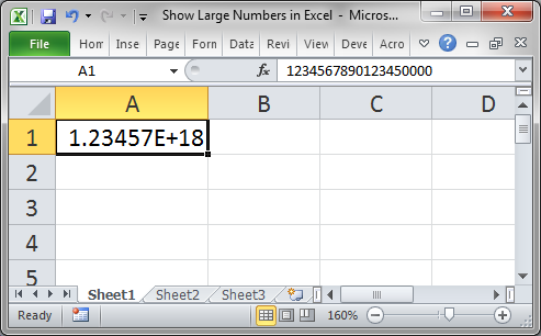
The number is represented in scientific notation but, look to the formula bar and you will see that the last 4 digits have been turned into zeros:
The Solution
Convert the number to text. You can do this by formatting a cell as Text before you put a number into it or by putting an apostrophe, same as a single quote, in front of the number.
Apostrophe Method
Input the number with a leading apostrophe like this:
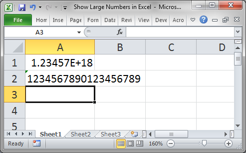
It’s as simple as that.
Format as Text Method
Select the cell where you want to input the number and then go to the Home tab and select Text from the Number drop down menu:
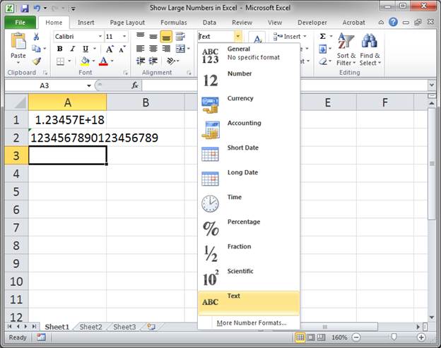
Input the number in that cell and that’s it:
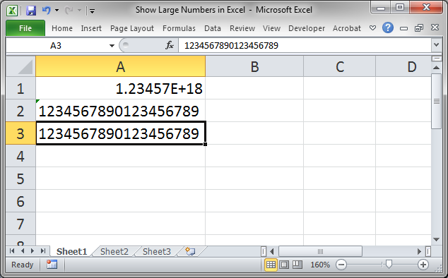
Important Note
When you store numbers as text, you cannot then perform the same types of calculations on it as you could if it was stored as a regular number. If you try to perform calculations on this number, you will notice that the results will not be as accurate as you predict because, no matter what, Excel will still cut-off the end of the number and replace it with zeros.
Displaying numbers like this is only good for displaying the numbers. Just because you can see the full number does not mean that you can perform accurate calculations with it.
Excel Number Limitations
Number Precision: 15 digits
Smallest Allowed Negative Number: -2.2251E-308
Smallest Allowed Positive Number: 2.2251E-308
Larges Allowed Negative Number: —9.99999999999999E+307
Larges Allowed Positive Number: 9.99999999999999E+307
Don’t forget to download the accompanying workbook so you can see the above examples in Excel.
Similar Content on TeachExcel
Convert Numbers Stored as Text to Numbers in Excel
Tutorial:
I’ll show you 4 ways to convert numbers stored as text to numbers in Excel. This situat…
Format Cells as a Scientific Number in Excel Number Formatting
Macro: This free Excel macro formats selected cells in the Scientific number format in Excel. Thi…
Keep Leading Zeros in Numbers in Excel — 2 Ways
Tutorial:
I’ll show you 2 ways to add and keep leading zeros in front of numbers in Excel.
These t…
Determine a Cell’s Color with this UDF — Outputs as Text or the Index Number in Excel
Macro: This free Excel UDF allows you to output the color of a cell in text format or as that col…
Quickly Create a Huge List of Numbers in Excel
Tutorial:
Quickly create a large list of numbers in Excel using the Fill Command. This will save …
Join a Date and Time into a Single Cell using VBA Macros in Excel
Tutorial: In order to combine a cell that has a date with a cell that has a time, using a Macro and …
Subscribe for Weekly Tutorials
BONUS: subscribe now to download our Top Tutorials Ebook!
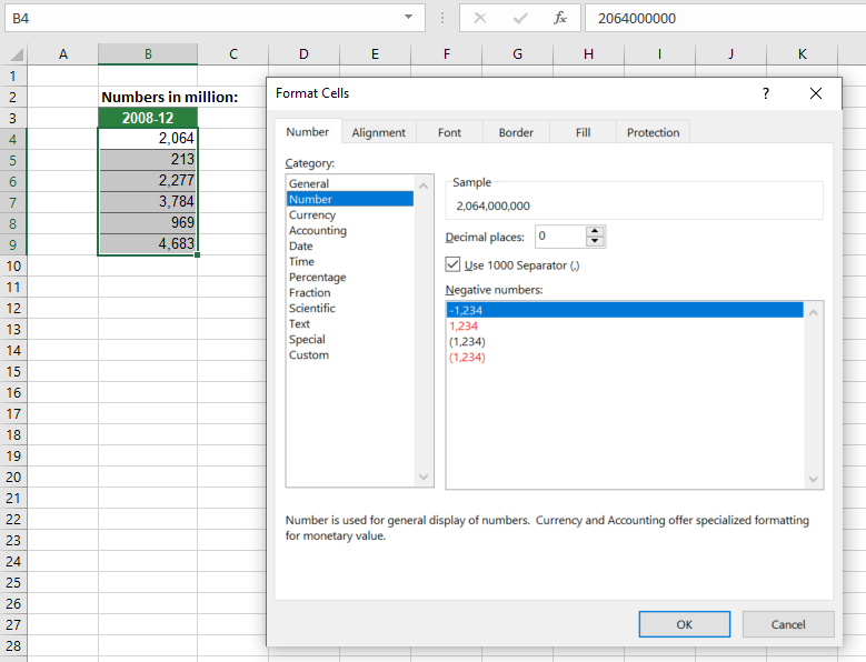
When you calculate with large numbers in Excel, you might want to only show the values as thousands or millions. 2,000 should be shown as 2. Unfortunately, Excel doesn’t offer such option with a single click. In this article you learn how to display numbers as thousands or millions by creating a custom number format.
In a hurry? Copy this for thousands #,##0,;-#,##0, and this for millions #,##0,,;-#,##0,, and paste it into the custom number format field.
Ways of displaying thousands and millions
There are different ways for achieving your desired number format
The first option would be dividing the results by thousands. This solution is easy to handle, but prone to errors. If you really want to use this method, please check out this article.
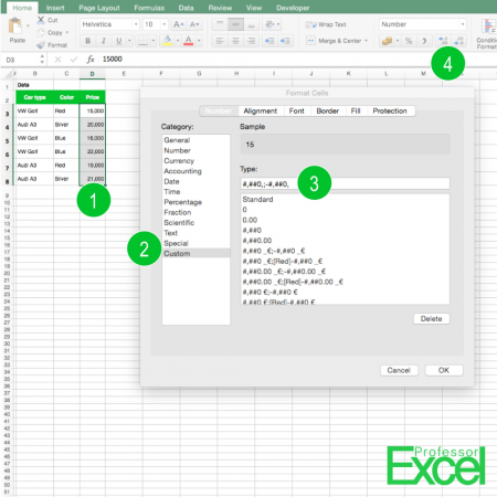
A better way is not changing the values, but only displaying them as thousands. Therefore, you have to define a custom number format (the numbers are corresponding with the picture):
- Select the cells which you want to display in thousands.
- Open the format cell dialogue by pressing Ctrl + 1 or right-click on the cell and select “Format Cells”. On the “Number” tab, click on “Custom” on the left hand side.
- For “Type” write: #,##0,;-#,##0, and confirm with OK.
# and 0 are placeholders for numbers (0 is always shown, no matter if there is a digit to display, whereas # is only shown when there is a number) and , (comma) stands for thousand separators. If you want to add a decimal separator, add a . (dot).
Once you’ve set up your format, you can also use the increase and decrease decimal buttons for displaying more or less digits (4). To display millions, use this code: #,##0,,;-#,##0,, (just one more comma).
You want to know more about custom format codes in Excel? Great – we have summarized everything you need to know here!
Do you want to boost your productivity in Excel?
Get the Professor Excel ribbon!

Add more than 120 great features to Excel!
Format codes for thousands and millions in Excel
- Thousands number format:
#,##0,;-#,##0,
- Millions number format:
#,##0,,;-#,##0,,
- Billions number format:
#,##0,,,;-#,##0,,,
If you work on a computer with a point as thousands separator: Replace the 3 commas of the billions number format with points.
Revert thousands and millions back to normal numbers
Because this was asked multiple times in the comments, let me quickly show how to revert thousands and millions back to normal numbers. It’s actually quite straight-forward:
- Select the cells you have formatted in thousands and millions and you want to get back to normal numbers.
- Press Ctrl + 1 on the keyboard. The Format Cells window opens.
- Go to the Number tab and select Number on the left-hand side. Define the desired number format.
If this doesn’t work it probably means that the underlying number is
- either not a number (text, e.g.)
- or not in thousands.
If it’s not a numeric value, you’ll probably need to work more on it (please see this article). If it’s just not in k, dividing or multiplying by 1000 might help.
Expert tip: Number formatting with Professor Excel Tools
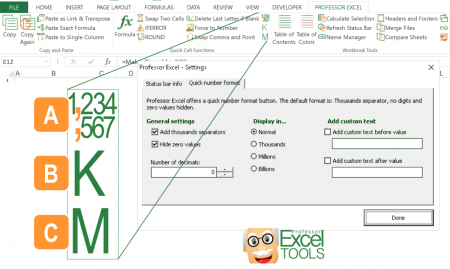
Another way of quickly formatting number is provided with ‘Professor Excel Tools‘. The Excel add-in offers three buttons for one-click-formatting options:
A: You can either define your favorite number preferences within the settings or use the two pre-formatted buttons. That way, you don’t have to remember any codes but just select your cell ranges and click the button for the desired cell format.
B: Format as thousands with just one click. Select the numbers to format and click this button.
C: Format as thousands with just one click. Select the numbers to format and click this button.
Try ‘Professor Excel Tools‘ for free and get to know all the amazing features. Download it by clicking the button below (no sign-up, no installation).

This function is included in our Excel Add-In ‘Professor Excel Tools’
(No sign-up, download starts directly)
Image by Eak K. from Pixabay
Numbers containing more than 15 digits in Excel are not often used, however some users might use them when recording credit card numbers, account numbers, stock codes, etc.
Applies To: Microsoft® Excel® for Windows 2013 and 2016.
Excel can’t handle more than 15 digits per cell, and so when these numbers are entered, Excel stores the first 15 digits and replaces all remaining digits with zeros.
For example; the number 1234567891234567 is stored as 1234567891234560


As these large numbers are NOT going to be used in a calculation, the issue is easily resolved, by simply formatting the cell to Text before entering the numbers.
Here’s how to do it:
- Select the cells of the columns where the numbers will be stored.
- On the Home tab, select the Number Format drop-down.

- Scroll all the way to the bottom of the list and select Text.

- Enter required numbers as usual.

A note to remember: if you copy and paste numbers from a different area to these formatted cells, you’ll need to use Paste Special Values or Paste as Text to retain the Text format in the cells. However, if used correctly, this will enable you to use more than 15 digits in Excel.
My clients keep asking me to display large numbers like in Thousands or Million to display in a shorter form. In the business world, K or M are used to represent Thousands or Millions.
For my own small Training business, I haven’t reached the revenue target of Million Dollar Sales…
But yes, I do achieve sales of several thousand from my blogs each month (PMChamp & ExcelChamp) and my Training company in Singapore & SkillsFuture Training Courses in Singapore.

However, my clients are usually small and medium enterprises as well as Multi-national companies, whose revenue is usually in Millions and sometimes in Billions too 🙂
Difficult to Read, Large Numbers look ugly in Excel
The problem is that for some people, it becomes difficult to read numbers and figures in Thousands, Millions and Billions, with so many zeroes to count.
And for our neighbouring country Indonesia, the currency denomination is so small, that a rent of a one-room apartment in Jakarta may be anywhere from 5 million to 10 million Indonesian Rupiah. So you can easily imagine how doing a simple budgeting exercise can take you into dizzying heights of billions and trillions.
How To Add a Thousand or Million Suffix to Numbers in Excel
For huge numbers, it is easier to read $23M or $25K rather than $23,000,000 or $23,000.
So let’s see how you can convert a large number in Thousands, Millions or Billions to be an easy to read number with Microsoft Excel.
- Simply select the number cell, or a range of numbers that you would like to convert into K or M.
- Right Click, and choose Custom Formatting.
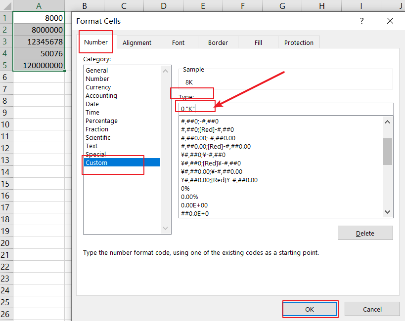
You can also choose Number Formatting from the Home Ribbon, or simply press the shortcut [Ctrl] + 1. - Go to Custom, and key in 0, “K” in the place where it says General. Now close the Format Cells popup window.
 Custom Number Format Popup in Microsoft Excel
 - Voila! Now your large number will be displayed in Thousands. So 23000 becomes 23K.
 Custom Number Format Popup in Microsoft Excel
How To Display Numbers in Millions in Excel
- Right-Click any number you want to convert. Go to Format Cells. In the pop-up window, move to Custom formatting.
- If you want to show the numbers in Millions, simply change the format from General to 0,,”M”. The figures will now be 23M. So essentially we are adding 2 commas instead of a single comma this time.
- If you would like to see the decimal point for the millions figure, like 23.6M, you can format it to 0.0,,”M”
- What’s great is that if you now create a chart on this data, the chart or Pivot Table will now show the figure in this custom format.
- Thus you will see the chart displaying numbers in Millions, or Thousands… saving space, and making the chart or pivot easier to read and analyze.
That’s it! Spend more time analyzing, not staring at the huge numbers 😉
You can check this out for yourself, by downloading the Sample Excel File. It has a few scenarios where you can try to convert large numbers into Millions or Thousands, whatever you prefer.
Sample Excel File Download: Number_formatting_in_K_or_M.xlsx
This technique applies to Excel 2003, Excel 2007, Excel 2010, Excel 2013, Excel 2016, Excel 2019 & Microsoft Office 365 editions.
It would work in all versions of Microsoft Excel in the past 20 years…
Hope it helps! Do share it with others on Facebook or LinkedIn.
And do comment or write to tell me of any issues you are facing in using Excel every day. There may be a simple solution that can save you a lot of time. At ExcelChamp, I solve many small problems each day to make Excel easy for everyone.
Cheers
Vinai Prakash
Need Tips on Pivot Tables, Data Analysis or Creating Better Charts?
Do checkout these resources
- How To Show Values and Percentages in Excel Pivot Tables
- 7 Habits of Highly Effective Data Analysts
- Creating Beautiful Excel Charts For Business Presentations
- Master Excel Lookup Functions like VLOOKUP, HLOOKUP, INDEX, MATCH, OFFSET
- FREE COURSE ON PIVOT TABLES TO ANALYZE DATA – No Signup is required. Click & Start watching Videos For Free and improve your Pivot Table Skills.
And if you want to learn Advanced Excel fast, then check out our detailed guide. Plus Master Lookup Functions like VLOOKUP, HLOOKUP, INDEX in Excel.
FREE COURSE ON PIVOT TABLES TO ANALYZE DATA – Click & Start watching Videos For Free and improve your Pivot Table Skills. No signup is required.
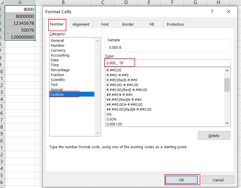
This post will guide you how to format numbers into thousands or millions or billions with Format Cells function in Excel 2013/2016. How do I format large numbers with Thousands or Millions separators in Excel.
For example, number 8000 should be shown as 8 or 8K, 8000000 should be shown as 8 or 8M. and Excel does not provide such option with a single click or way. And you can use number formatting feature to achieve the result.
Excel Number Formatting is a larger feature in Excel, and we have written lots of posts which includes all kinds of number formatting in Excel. Number Formatting allows you to modify the appearance of cell values without changing their real values. Also you can also add Thousands or Millions separators without changing the cell actual values.
In Microsoft Excel, if you want to improve the readability of your data by formatting numbers to show as thousands(k), Millions(M), or Billions(B). The below steps will show you how to format numbers with Thousands or Millions separators to show in a shorter format to read and understand very easily by creating a custom number format.
Table of Contents
- Format Numbers in Thousands
- Format Numbers in Thousands with Formula
- Format Numbers in Millions
- Format Numbers in Billions
- Format Numbers in Thousands, Millions, Billions Based on Numbers
Firstly, we will show you how to format numbers in thousands by create a custom format with the Format Cells function in your worksheet.
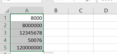
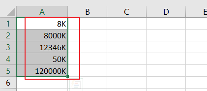
Assuming that you have a list of data with the below set of numbers in cell range A1:A5. And now we need to format these numbers in thousands.
Just do the following steps to change the formatting of the numbers:
Step1: select your numbers in range A1:A5.
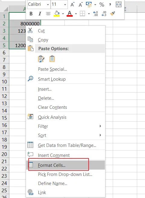
Step2: right click on the selected cells that you want to format. and select Format Cells menu from the pop-up menu list. And the Format Cell dialog box will appear. Or you can also press the shortcut key CTRL +1 to open the Format Cells dialog box.
Step3: click Number tab in the Format Cells dialog box, and click the Custom option from the left pane.
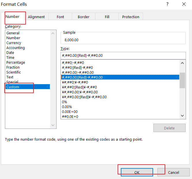
Step4: now go to Type: section in the Format Cells dialog box, add the following formatting code to change the formatting of the selected numbers. Click Ok button.
0, "K"
Or
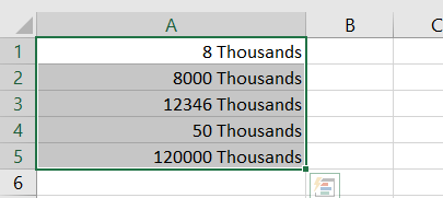
0, “ Thousands”
Step5: your selected numbers will appear in thousands automatically. And the formatting does not change the integrity or truncate your numeric values in any way. And it will apply a cosmetic effect to the number.
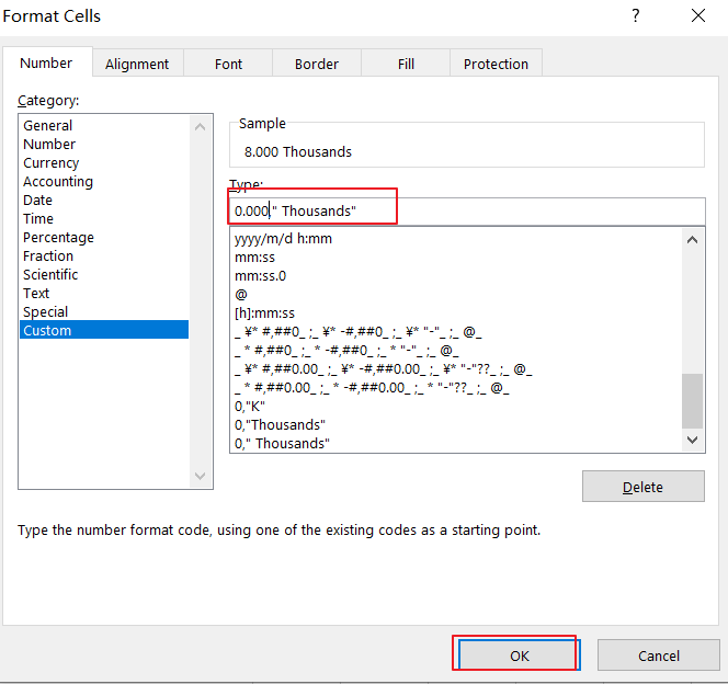
If you want to show the exact value, and you can change the formatting code as below:
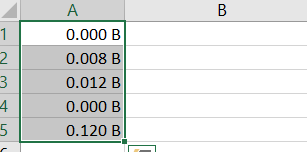
0.000,”K”
Or
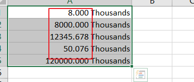
0.000,” Thousands”
Then you will see that the exact values with decimal points should be shown.
Format Numbers in Thousands with Formula
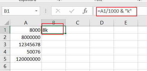
There is another method to format numbers in thousands separator in Excel. And you can create a formula based on concentrate character. You need to divide the number by 1000 and combine the word “Thousands” or character “K” by using concentrate character “&”. Type the following formula in a blank cell:
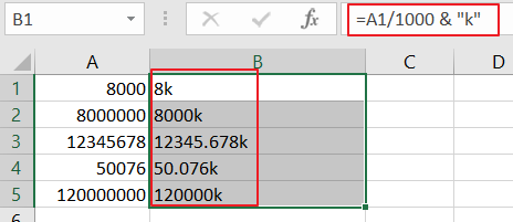
=A1/1000 & “K”
Or
=A1/1000 & “ Thousand”
Then you can drag the Fill Handle down to other cells to apply this formula.
Format Numbers in Millions
The above steps have shown you how to format numbers in thousands, and the below steps will show you how to format number in Millions. Just do the following steps:
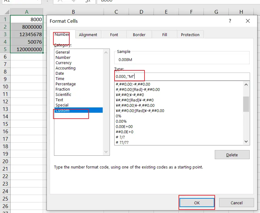
Step1: open the Format Cells dialog box, and click the Custom option.
Step2: add the following format code in the Type: section. The only difference between previous code and this format code is that you need to add one extra comma(,).
0.000,, “M”
Or
0.000,, “ Million”
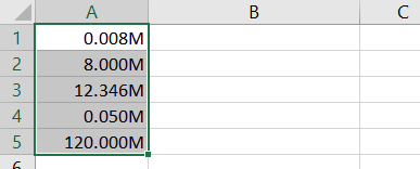
Step3: the result is as below:
Format Numbers in Billions
In the previous step we have talked that how to format numbers in thousands and millions. And now we will see that how to format numbers in Billions.
You just need to refer to the above steps, and then use another format code to change the formatting of the numbers in Billions.
0.000,,, “B”
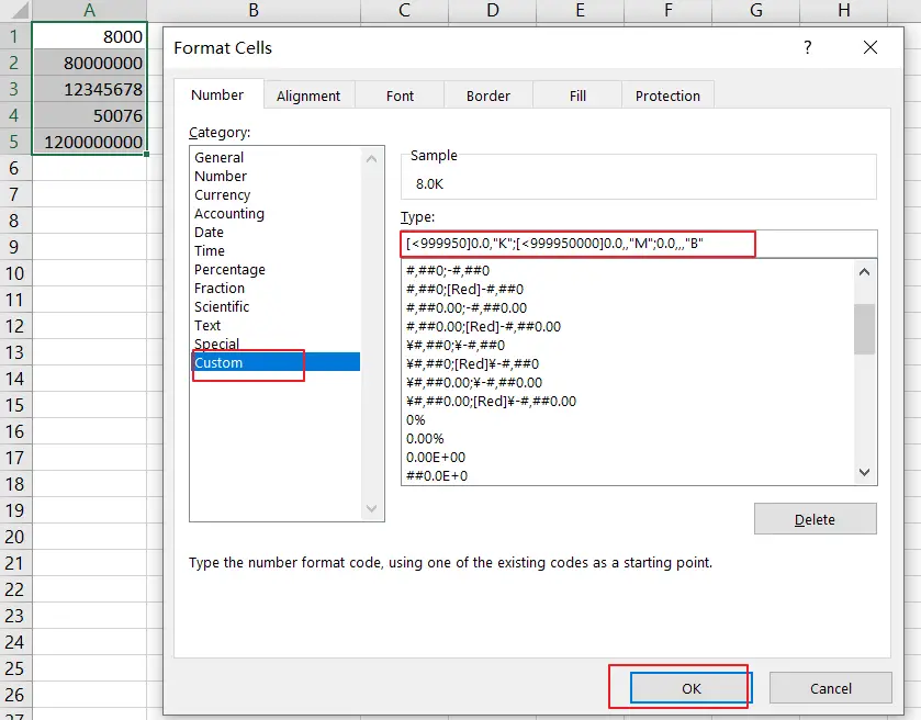
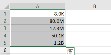
Format Numbers in Thousands, Millions, Billions Based on Numbers
If you want to format numbers to show the result based on the cell values. For example, if the cell value is less than 10000, and the result display as 10K, and if the cell value is greater than or equal to 1000000, then the result is displayed in Million. You can add the following format code into Type: section.
[<999950]0.0,"K";[<999950000]0.0,,"M";0.0,,,"B"
Improve Article
Save Article
Like Article
Improve Article
Save Article
Like Article
By default, in the cells of an Excel sheet, we canter 11 digits maximum. Once we enter a 12-digit number Excel changes it in terms of exponent and power notation.
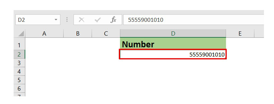
11 digit number
Now, if we enter a 12 digit number let’s see what happens.
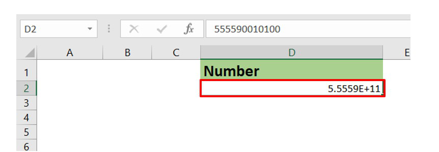
We can observe that the representation of the 12-digit number becomes in terms of the power of 10 by converting to a decimal form. This is not a good representation since we can’t get the accurate precision of the number from the above representation.
In real life many times we deal with numbers having more than 11 digits. A great example is our Credit Card number which consists of 16 digits. So, we need an alternate way in Excel to store our Credit Card number with all the digits visible instead of decimal representation.
In this article, we are going to see how to enter large numbers in Excel using a credit card number having 16 digits as an example.
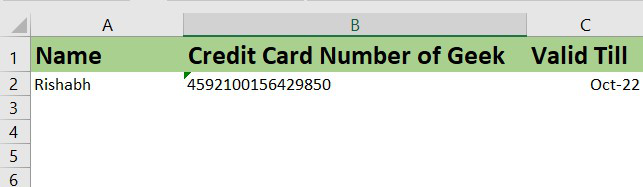
Example: Consider the dataset having the name, credit card number, expiry date of a geek.
Insert the data in the worksheet as shown below :
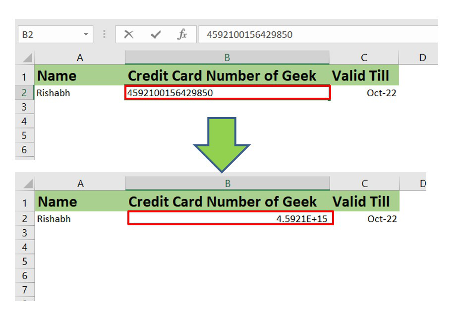
We can observe as we enter the 16-digit number in the worksheet Excel automatically converts it into a decimal form.
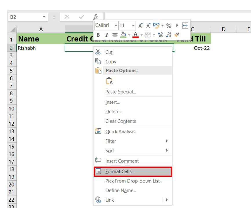
So, to avoid it an alternate technique is there. The steps are :
- Right-click on the cell where you want to add a large number.
- A menu appears. Click on the Format Cells option.
- The Format Cells dialog box opens. In this click on the Number tab.
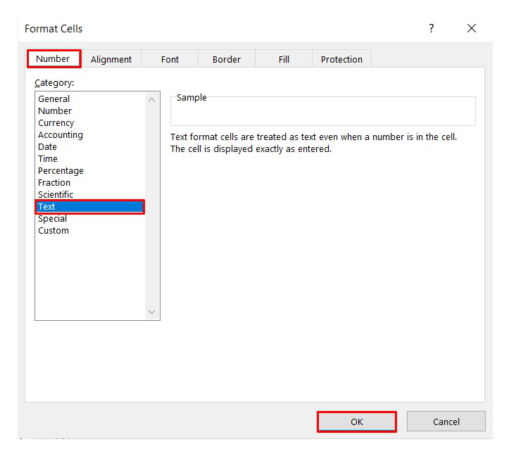
- Now in the Category options select the Text option. This will format the cell from a number to a text. And we know a single Excel cell can read up to 32,767 characters in maximum. This will now prohibit the conversion of the credit card number into decimal form. This formatting will now consider each digit as a character.
- Click OK.
- Now re-enter the credit card number again and this time we will observe that we get the exact number and every digit is visible (with 100% precision) in the 16-digit number.
In this way you can store a number in Excel containing more than 11 digits. It is a prediction that in upcoming updated versions of Excel, Microsoft will increase the limit up to 16 digits so that a credit card number can be stored easily without any formatting.
Like Article
Save Article