
Были ли сведения полезными?
(Чем больше вы сообщите нам, тем больше вероятность, что мы вам поможем.)
(Чем больше вы сообщите нам, тем больше вероятность, что мы вам поможем.)
Насколько вы удовлетворены качеством перевода?
Что повлияло на вашу оценку?
Моя проблема решена
Понятные инструкции
Понятные сведения
Без профессиональной лексики
Полезные изображения
Качество перевода
Не соответствует интерфейсу
Неверные инструкции
Слишком техническая информация
Недостаточно информации
Недостаточно изображений
Качество перевода
Добавите что-нибудь? Это необязательно
Спасибо за ваш отзыв!
×
![]()
Download Article
Display your Excel data in a colorful pie chart with this simple guide
![]()
Download Article
- Preparing the Data
- Creating a Chart
- Formatting Your Pie Chart
- Q&A
- Tips
|
|
|
|
Do you want to create a pie chart in Microsoft Excel? You can make 2-D and 3-D pie charts for your data and customize it using Excel’s Chart Elements. This is a great way to organize and display data as a percentage of a whole. This wikiHow will show you how to create a visual representation of your data in Microsoft Excel using a pie chart on your Windows or Mac computer.
Things You Should Know
- You need to prepare your chart data in Excel before creating a chart.
- To make a pie chart, select your data. Click Insert and click the Pie chart icon. Select 2-D or 3-D Pie Chart.
- Customize your pie chart’s colors by using the Chart Elements tab. Click the chart to customize displayed data.
-

1
-
2
Add a name to the chart. To do so, click the B1 cell and then type in the chart’s name.
- For example, if you’re making a chart about your budget, the B1 cell should say something like «2022 Budget».
- You can also type in a clarifying label—e.g., «Budget Allocation»—in the A1 cell.
Advertisement
-
3
Add your data to the chart. You’ll place prospective pie chart sections’ labels in the A column and those sections’ values in the B column.
- For the budget example above, you might write «Car Expenses» in A2 and then put «$1000» in B2.
- The pie chart template will automatically determine percentages for you.
-
4
Finish adding your data. Once you’ve completed this process, you’re ready to create a pie chart using your data.


Advertisement
-
1
Select all of your data. To do so, click the A1 cell, hold down the Shift key, and then click the bottom value in the B column. This will select all of your data.[1]
- If your chart uses different column letters, numbers, and so on, simply remember to click the top-left cell in your data group and then click the bottom-right while holding the Shift key.
-
2
Click the Insert tab. It’s at the top of the Excel window, to the right of the Home tab.[2]
-
3
Click the «Pie Chart» icon. This is a circular button in the «Charts» group of options, which is below and to the right of the Insert tab. You’ll see several options appear in a drop-down menu:
- 2-D Pie: Create a simple pie chart that displays color-coded sections of your data.
- 3-D Pie: Uses a three-dimensional pie chart that displays color-coded data.
- Donut: Displays color-coded data with a hole in the center for series of data.
- You can also click More Pie Charts… to view all available options.
-
4
Click a chart option. Doing so will create a pie chart with your data applied to it; you should see color-coded tabs at the bottom of the chart that correspond to the colored sections of the chart itself.
- You can preview options here by hovering your mouse over the different chart templates.


Advertisement
-
1
Click Chart Design. This is the tab on the top toolbar, next to Help and Format. You’ll be able to change the way your graph looks, including the color schemes used, the text allocation, and whether or not percentages are displayed.
- If you don’t see this tab, you’ll need to click on your chart first.
-
2
Change your chart style. Switch between styles by clicking the previews above Chart Styles.
- Only one style preset can be applied at a time.
- You can also click the paintbrush icon next to the chart to find Chart Styles in the Styles tab.
-
3
Change your chart color. Click the Change Colors icon. This looks like a color palette. A drop-down menu will appear with multiple color themes listed.
- Click the color scheme you want to apply.
- You can also click the paintbrush icon next to the chart and click the Color tab to change your chart colors.
-
4
Toggle chart labels. Click your chart, then click the + from the side icons.
- To remove data and percentage labels from your chart, uncheck Data Labels underneath Chart Elements.
- To remove category or percentage labels separately, click the arrow next to Data Labels, then More Options. Use the right panel to uncheck Percentage or Category name.
-
5
Customize the Chart Area. With the chart selected, the Format Chart Area will be visible in the right panel.
- Fill & Line: Customize Fill and Border options.
- Effects: Add effects such as Shadow, Glow, Soft Edges, and 3-D Format.
- Size & Properties: Customize the height, width, and scale of your chart.


Advertisement
Add New Question
-
Question
How do I create a pie chart without percentages?

You’ll have to make percentages. A pie chart by definition is 100%. If your data is not in percent, then Excel will create percentages for you.
-
Question
How do I change the color of the pie chart?
Once you have the pie chart on the board, there are different shades next to it that says «change color»; click on that.
-
Question
What am I doing wrong if I tried this method and the pie chart didn’t show up?
You might have entered information wrongly and it can’t process. Try re-entering your data.
See more answers
Ask a Question
200 characters left
Include your email address to get a message when this question is answered.
Submit
Advertisement
-
You can copy your chart and paste it into other Microsoft Office products (e.g., Word or PowerPoint).
-
If you want to create charts for multiple sets of data, repeat this process for each set. Once the chart appears, click and drag it away from the center of the Excel document to prevent it from covering up your first chart.
-
Looking for money-saving deals on Microsoft Office products like Excel? Check out our coupon site for tons of coupons and promo codes on your next subscription.
Thanks for submitting a tip for review!
Advertisement
About This Article
Article SummaryX
1. Open Excel.
2. Enter your data.
3. Select all of your data.
4. Click the Insert tab.
5. Click the «Pie Chart» icon.
6. Click a pie chart template.
Did this summary help you?
Thanks to all authors for creating a page that has been read 1,059,805 times.
Is this article up to date?
Круговая диаграмма, построенная в документе Microsoft Excel, предоставляет многогранную информацию для восприятия. Если в табличном формате изучить ее сложнее, то в виде диаграммы все становится наглядным. В этой статье рассмотрим, что такое круговая диаграмма и как построить ее при помощи Excel.
Что такое круговая диаграммы и ее типы
Диаграмма кругового или секторного типа представляет графический объект, который отражает информацию, указанную в процентном эквиваленте. Существует несколько типов оформления секторных диаграмм:
- объемная,
- вторичная,
- кольцевая.
Каждый из предложенных вариантов отличается внешним видом и особенностями форматирования.
Как построить круговую диаграмму: начинаем с азов
Если ответственно отнестись к инструкции, построение диаграммы не займет времени. Главное, чтобы данные в таблицах были указаны верно.
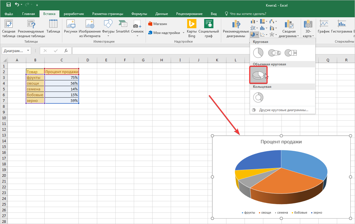
- Убедитесь, что вся информация указана, только после этого приступайте к вставке объекта. Для этого перейдите во вкладку «Вставка», найдите блок «Диаграмма» и кликните «Круговая диаграмма».
- Перед вами открывается меню с доступными вариантами круговых диаграмм. Для примера выберем объемный тип. После этого на листе рядом с таблицей у вас добавится новый объект с учетом данных в процентном эквиваленте.
Для построения кругового типа диаграмм все значения в таблице обязательно должны быть больше нуля. Иначе графическое изображение будет отображаться с ошибками.
- В заданном случае необходимо не только визуально отобразить количество процентов, но и указать их в виде подписи на каждом секторе. Чтобы оформить объект таким образом, необходимо в открывшемся «Конструкторе диаграмм» выбрать вариант стиля № 3 с указанием чисел прямо на диаграмме.
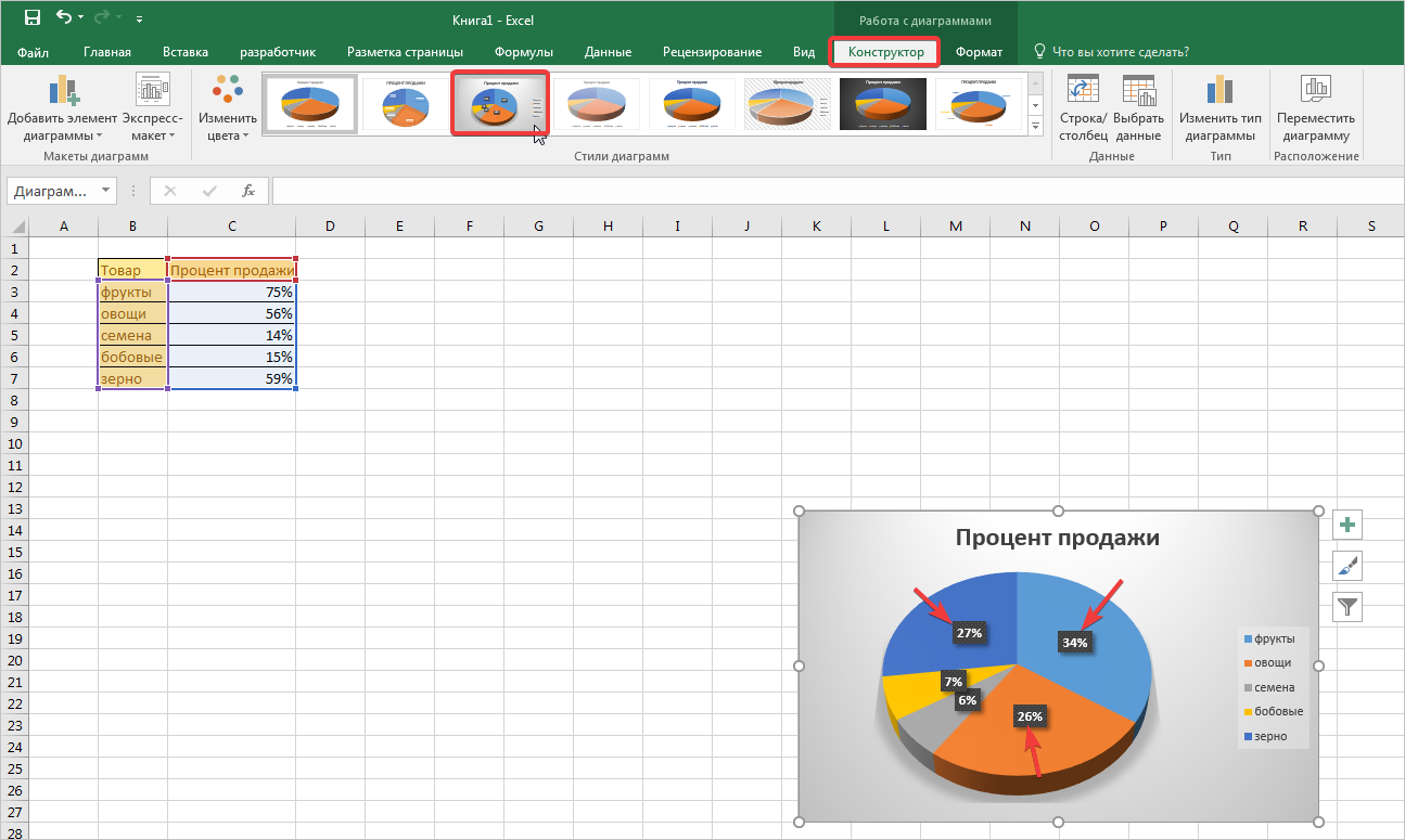
- Обратите внимание на фото, все необходимые проценты скопировались из таблицы на диаграмму.
Простой способ разделить круговую диаграмму на сектора
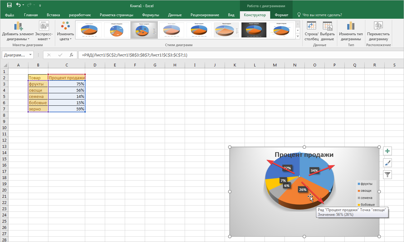
Один из элементарных методов разбить диаграмму на несколько секторов с целью их выделения — это перетаскивание мышью. Чтобы это выполнить, проводим следующие манипуляции.
- Кликаем мышью по объекту дважды. Вы увидите, что диаграмма активировалась. После этого оттягиваем нужные сектора от центра, чтобы визуально выделить.
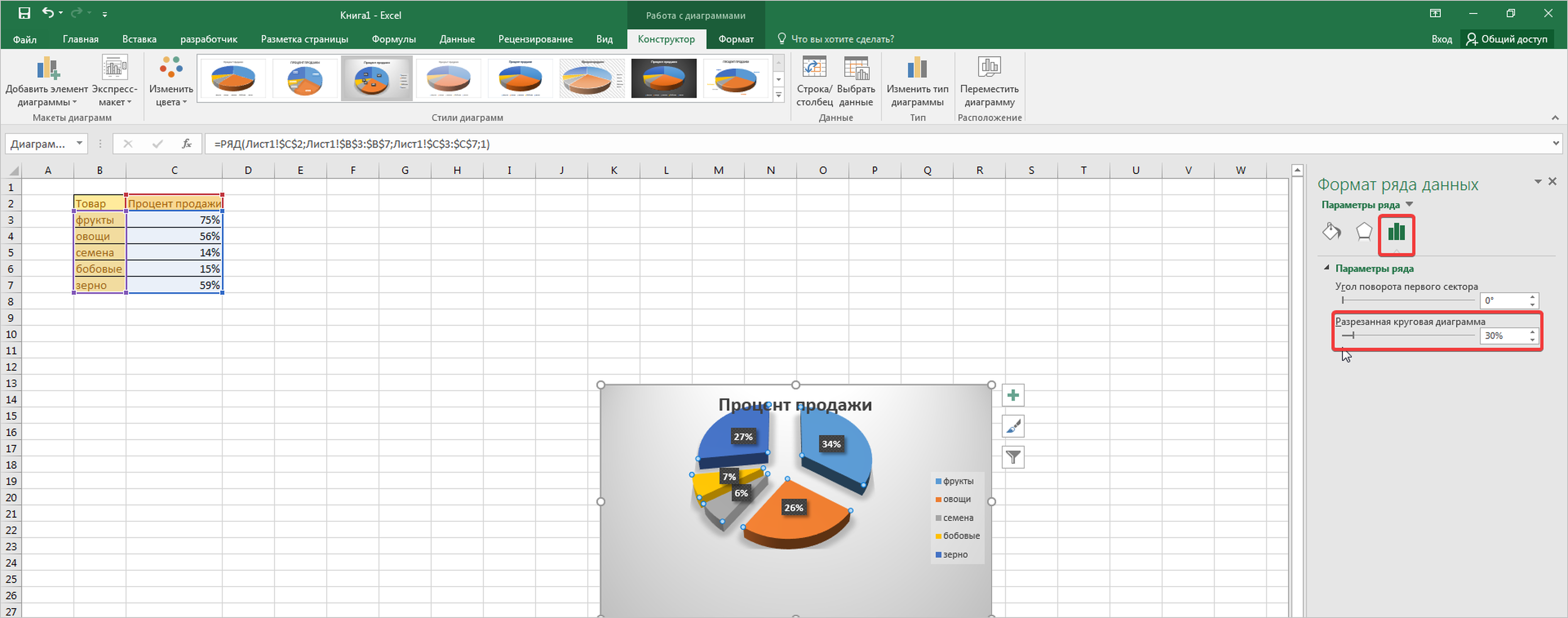
- Также вы можете использовать специальное меню. Чтобы его вызвать, сделайте двойной клик по секторам, и справа от таблицы откроется небольшое меню настроек.
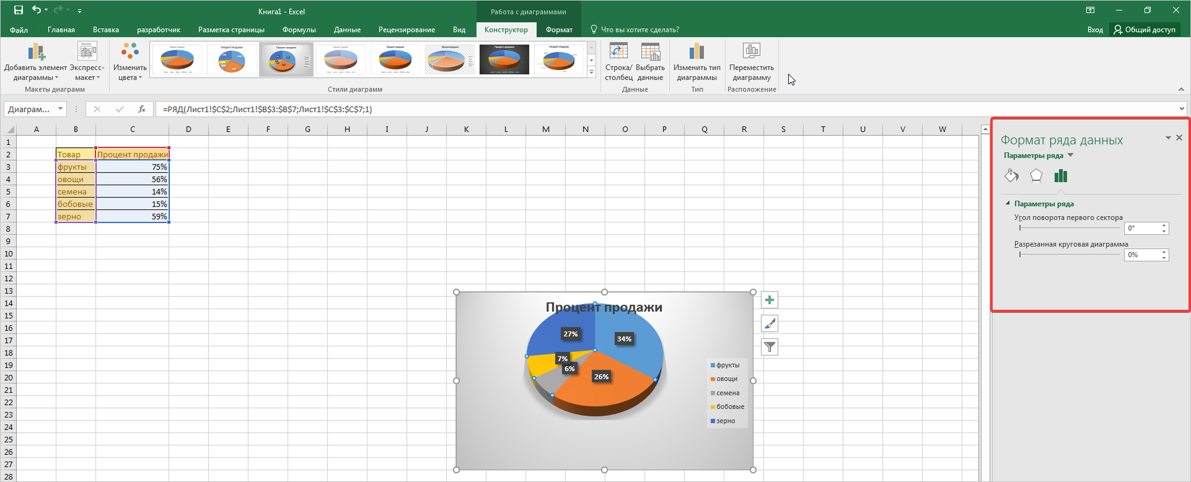
- Здесь переходим в пункт «Параметры ряда» и меняем процент разрезной диаграммы до оптимальных значений. Также для привлекательности можно поменять и угол поворота выделенного сектора или вынести его вверх.
Для корректного отображения данных в секторной диаграмме, категорий с процентными данными должно быть не больше 7. Если их больше, то все сектора будут показаны размытыми.
Кроме этих манипуляций, вы можете использовать и другие с целью форматирования секторных диаграмм. Аналогичными способами редактируются и другие типы объектов с информацией в процентах.