
This tutorial will demonstrate ho to perform the Shapiro-Wilk test in Excel and Google Sheets.
Shapiro-Wilk test is a statistical test conducted to determine whether a dataset can be modeled using the normal distribution, and thus, whether a randomly selected subset of the dataset can be said to be normally distributed. The Shapiro-Wilk test is considered one of the best among the numerical methods of testing for normality because of its high statistical power.
The original Shapiro-Wilk test, like most significance tests, is affected by the sample size and works best for sample sizes of n=2 to n=50. For larger sample sizes (up to n=2000), an extension of the Shapiro-Wilk test called the Shapiro-Wilk Royston test can be used.
How Shapiro-Wilk Test Works
The Shapiro-Wilk test tests the null hypothesis that the dataset comes from a normally distributed population against the alternative hypothesis that the dataset does not come from a normally distributed population.
The test statistics for the Shapiro-Wilk test is given as follows:
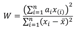
where x(i) is the ith order statistic (i.e. the ith data value after the dataset is arranged in ascending order),
![]() is the mean (average) of the dataset.
is the mean (average) of the dataset.
n is the number of data points in the dataset, and
a = [ai] = (a1,…,an ) is the coefficient vector of the weights of the Shapiro-Wilk test (obtained from the Shapiro-Wilk test table),
The vector a is anti-symmetric, that is a n+1-i =-ai for all i, and a(n+1)/2 = 0 for odd n. Also, aT a = 1.
The p-value is obtained by comparing the W statistic with the W values presented in the Shapiro-Wilk test table of p-values for the given sample size.
- If the obtained -value is less than the chosen significance level, the null hypothesis is rejected, and it is concluded that the dataset is not from a normally distributed population,
- Otherwise, the null hypothesis is not rejected and it is concluded that there is no statistically significant evidence that the dataset does not come from a normally distributed population.
How to Perform the Shapiro-Wilk Test in Excel
Background: A sample of the heights, in inches, of 14 ten years old boys are presented in the table below. Use the Shapiro-Wilk method of testing for normality to test whether the data obtained from the sample can be modeled using a normal distribution.
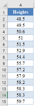
First, select the values in the dataset and Sort the data using the Sort tool: Data > Sort (Sort Smallest to Largest)

This will sort the values like so:
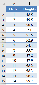
Alternatively, with newer versions of Excel, you can use the SORT Function to sort the data:
=SORT(B2:B15)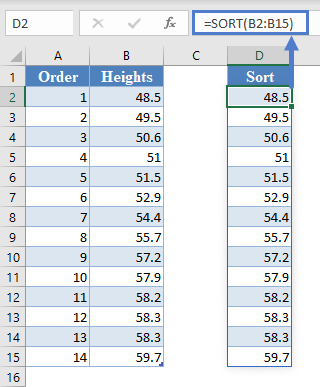
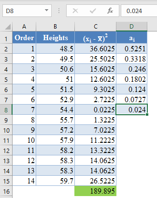
Next, calculate the denominator of the W statistic, ![]() , as shown in the picture below, using AVERAGE to calculate the mean:
, as shown in the picture below, using AVERAGE to calculate the mean:
=(B2-AVERAGE($B$2:$B$15))^2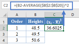
Complete the rest of the column and then calculate the sum (shown in green background) as shown in the picture below:
=SUM(C2:C15)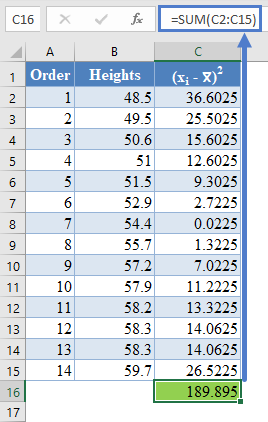
Thus, the denominator of the W statistic is 189.895.
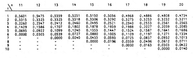
Next, obtain the values of ai , the coefficients of the weights of the Shapiro-Wilk test, for a sample size of n=14 from the Shapiro-Wilk test table. An excerpt of the Shapiro-Wilk test table is shown below:
These values will need to be entered manually as follows:
And using the anti-symmetric property of ai, that is, an+1-i=-ai for all i, we have that a14=-a1, a13=-a2, etc. So, the complete values of the ai column are shown in the picture below:
=-D8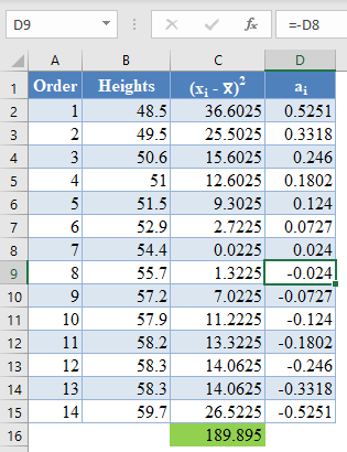
*Note that because of the anti-symmetric property of ai and since that numerator of the W statistic is a square, it does not matter which half of the ai column is positive or negative. That is, you can choose to make the upper half of the column to be positive and the lower half negative or vice-versa and it will not affect your final result.
Next, multiply the ai values with the corresponding (already arranged) values in the dataset to get the ai x(i) column. The calculation and the value for the first data point are shown in the picture below:
=D2*B2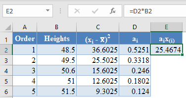
Complete the rest of the ai x(i) column and calculate the sum (shown in green background) as shown in the picture below:
=sum(E2:E15)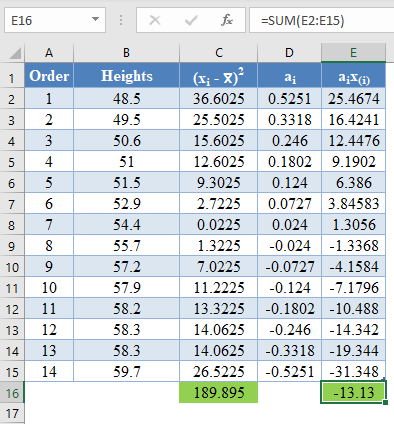
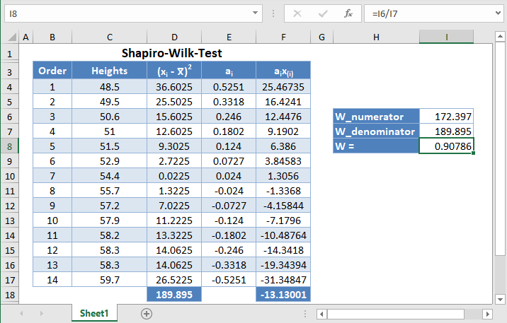
The denominator of the W statistic as obtained previously is 189.895 , and the numerator is the square of the sum of the ai x(i) column. Thus, we have as follows:
=E16^2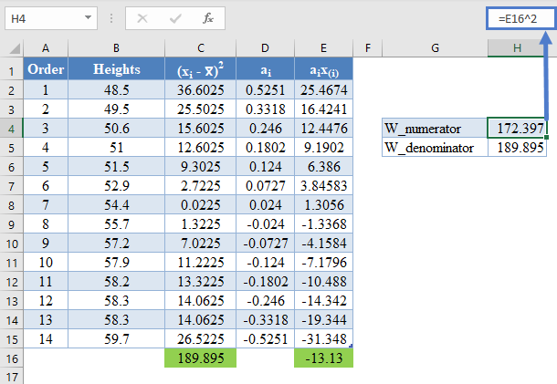
Therefore, the W statistic is as shown below:
=H4/H5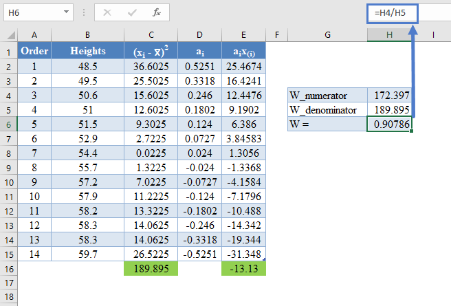
Finally, obtain the p-value of the test using the Shapiro-Wilk test table of p-values considering the sample size.
An excerpt of the Shapiro-Wilk test table of p-values is shown below:
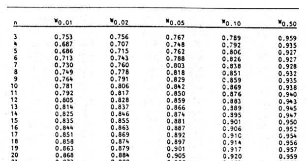
For this test, we will use a significance (alpha) level of 0.05. From the table, you can see that for n =14, W = 0.90786 is between W0.10 = 0.895 and W0.50 = 0.947, which means that the p-value is between 0.10 and 0.50. This means that the p-value is greater than α = 0.05, hence, the null hypothesis is not rejected.
Therefore, we conclude that there is not enough evidence that the dataset is not drawn from a normally distributed population. That is, we can assume that the dataset is normally distributed.
*Using linear interpolation, you can get that the approximate p-value is 0.1989.
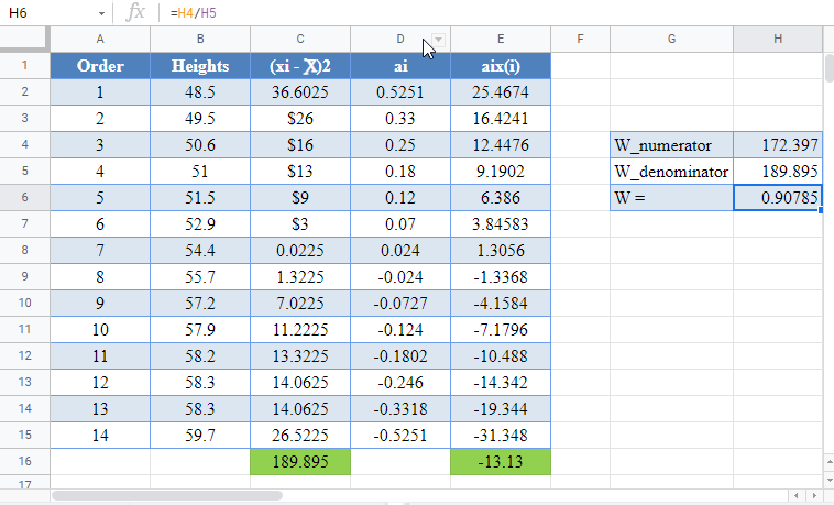
Shapiro-Wilk Test in Google Sheets
Shapiro-Wilk test can be conducted in Google Sheets in a similar way as done in Excel as shown in the picture below.
Basic Concepts
We present the original approach to performing the Shapiro-Wilk Test. This approach is limited to samples between 3 and 50 elements. By clicking here you can also review a revised approach using the algorithm of J. P. Royston which can handle samples with up to 5,000 (or even more).
The basic approach used in the Shapiro-Wilk (SW) test for normality is as follows:
- Arrange the data in ascending order so that x1 ≤ … ≤ xn.
- Calculate SS as follows:
![]()
- If n is even, let m = n/2, while if n is odd let m = (n–1)/2
- Calculate b as follows, taking the ai weights from Table 1 (based on the value of n) in the Shapiro-Wilk Tables. Note that if n is odd, the median data value is not used in the calculation of b.
![]()
- Calculate the test statistic W = b2 ⁄ SS
- Find the value in Table 2 of the Shapiro-Wilk Tables (for a given value of n) that is closest to W, interpolating if necessary. This is the p-value for the test.
For example, suppose W = .975 and n = 10. Based on Table 2 of the Shapiro-Wilk Tables the p-value for the test is somewhere between .90 (W = .972) and .95 (W = .978).
Examples
Example 1: A random sample of 12 people is taken from a large population. The ages of the people in the sample are shown in column A of the worksheet in Figure 1. Is this data normally distributed?

Figure 1 – Shapiro-Wilk test for Example 1
We begin by sorting the data in column A using Data > Sort & Filter|Sort (see Sorting and Filtering) or the Real Statistics QSORT function (see Sorting and Removing Duplicates), putting the results in column B. We next look up the coefficient values for n = 12 (the sample size) in Table 1 of the Shapiro-Wilk Tables, putting these values in column E.
Corresponding to each of these 6 coefficients a1,…,a6, we calculate the values x12 – x1, …, x7 – x6, where xi is the ith data element in sorted order. E.g. since x1 = 35 and x12 = 86, we place the difference 86 – 35 = 51 in cell H5 (the same row as the cell containing coefficient a1). Column I contains the product of the coefficients and difference values. E.g. cell I5 contains the formula =E5*H5. The sum of these values is b = 44.1641, which is found in cell I11 (and again in cell E14).
We next calculate SS as DEVSQ(B4:B15) = 2008.667 (cell E13). Thus W = b2 ⁄ SS = 44.1641^2/2008.667 = .971026 (cell E15). We now look for .971026 when n = 12 in Table 2 of the Shapiro-Wilk Tables and find that the p-value lies between .50 and .90. The W value for .5 is .943 and the W value for .9 is .973.
Interpolating .971026 between these value (using linear interpolation), we arrive at p-value = .873681. Since p-value = .87 > .05 = α, we retain the null hypothesis that the data are normally distributed. Since this p-value is based on linear interpolation, it is not very accurate, but the important thing is that it is much higher than the alpha value, and so we can retain the null hypothesis that the data is normally distributed.
Example 2: Using the SW test, determine whether the data in Example 1 of Graphical Tests for Normality and Symmetry (repeated in column A of Figure 2) are normally distributed.

Figure 2 – Shapiro-Wilk test for Example 2
As we can see from the analysis in Figure 2, p-value = .0432 < .05 = α, and so we reject the null hypothesis and conclude with 95% confidence that the data are not normally distributed, which is quite different from the results using the KS test that we found in Example 2 of Kolmogorov-Smironov Test, but consistent with the QQ plot shown in Figure 5 of that webpage.
Real Statistics Support
Real Statistics Function: The Real Statistics Resource Pack contains the following functions.
SHAPIRO(R1, FALSE) = the Shapiro-Wilk test statistic W for the data in R1
SWTEST(R1, FALSE, interp) = p-value of the Shapiro-Wilk test on the data in R1
SWCoeff(n, j, FALSE) = the jth coefficient for samples of size n
SWCoeff(R1, C1, FALSE) = the coefficient corresponding to cell C1 within sorted range R1
SWPROB(n, W, FALSE, interp) = p-value of the Shapiro-Wilk test for a sample of size n for test statistic W
The functions SHAPIRO and SWTEST ignore all empty and non-numeric cells. The range R1 in SWCoeff(R1, C1, FALSE) should not contain any empty or non-numeric cells.
When performing the table lookup, the default is to use the recommended type of interpolation (interp = TRUE). To use linear interpolation, set interp to FALSE. See Interpolation for details.
For Example 1 of Chi-square Test for Normality, SHAPIRO(A4:A15, FALSE) = .874 and SWTEST(A4:A15, FALSE, FALSE) = SWPROB(15,.874,FALSE,FALSE) = .0419 (referring to the worksheet in Figure 2 of Chi-square Test for Normality).
Note that SHAPIRO(R1, TRUE), SWTEST(R1, TRUE), SWCoeff(n, j, TRUE), SWCoeff(R1, C1, TRUE) and SWPROB(n, W, TRUE) refer to the results using the Royston algorithm, as described in Shapiro-Wilk Expanded Test.
For compatibility with the Royston version of SWCoeff, when j ≤ n/2 then SWCoeff(n, j, FALSE) = the negative of the value of the jth coefficient for samples of size n found in the Shapiro-Wilk Tables. When j = (n+1)/2, SWCoeff(n, j, FALSE) = 0 and when j > (n+1)/2, SWCoeff(n, j, FALSE) = -SWCoeff(n, n–j+1, FALSE).
Reference
Shapiro, S.S. & Wilk, M.B. (1965) An analysis of variance for normality (complete samples). Biometrika, Vol. 52, No. 3/4.
http://webspace.ship.edu/pgmarr/Geo441/Readings/Shapiro%20and%20Wilk%201965%20-%20An%20Analysis%20of%20Variance%20Test%20for%20Normality.pdf
Why do we need to run a normality test?
Normality tests enable you to know whether your dataset follows a normal distribution. Moreover, normality of residuals is a required assumption in common statistical modeling methods.
Normality tests involve the null hypothesis that the variable from which the sample is drawn follows a normal distribution. Thus, a low p-value indicates a low risk of being wrong when stating that the data are not normal. In other words, if p-value < alpha risk threshold, the data are significantly not normal.
How do normality tests work?
We calculate the test statistic below on our dataset :
W=(∑i=1naix(i))2∑i=1n(xi−xˉ)2W=dfrac{(sum_{i=1}^na_ix_{(i)})^2}{sum_{i=1}^n(x_i-bar{x})^2}
If its values are below the bounds defined in the Shapiro-Wilk table for a set alpha threshold, then the associated p-value is less than alpha and the null hypothesis is rejected and the data does not follow a normal distribution.
Dataset for Shapiro-Wilk and other normality tests
The data represent two samples each containing the average math score of 1000 students.
Setting up a Shapiro-Wilk and other normality tests
We then want to test the normality of the two samples. Select the XLSTAT / Describing data / Normality tests, or click on the corresponding button of the Describing data menu.

Once you’ve clicked on the button, the dialog box appears. Select the two samples in the Data field.
The Q-Q plot option is activated to allow us to visually check the normality of the samples.


The computations begin once you have clicked on the OK button, and the results are displayed on a new sheet.
Interpreting the results of a Shapiro-Wilk and other normality tests
The results are first displayed for the first sample and then for the second sample.
The first result displayed is the Q-Q plot for the first sample. The Q-Q plot allows us to compare the cumulative distribution function (cdf) of the sample (abscissa) to the cumulative distribution function of the normal distribution with the same mean and standard deviation (ordinates). In the case of a sample following a normal distribution, we should observe an alignment with the first bisecting line. In the other cases some deviations from the bisecting line should be observed.

We can see here that the empiric cdf is very close to the bisecting line. The Shapiro-Wilk and Jarque-Bera confirm that we cannot reject the normality assumption for the sample. We notice that with the Shapiro-Wilk test, the risk of being wrong when rejecting the null assumption is smaller than with the Jarque-Bera test.

The following results are for the second sample. Contrary to what we have observed for the first sample, we notice here on the Q-Q plot that there are two strong deviations indicating that the distribution is most probably not normal.

This gap is confirmed by the normality tests (see below) which allow us to assert with no hesitation that we need to reject the hypothesis that the sample might be normally distributed.

Conclusion
In conclusion, in this tutorial, we have seen how to test two samples for normality using Shapiro-Wilk and Jarque-Bera tests. These tests did not reject the normality assumption for the first sample and allowed us to reject it for the second sample.
Was this article useful?
- Yes
- No
Библиографическое описание:
Дручинин, Д. О. Проверка гипотезы о нормальном распределении логарифмической доходности по критерию Шапиро — Уилка / Д. О. Дручинин. — Текст : непосредственный // Молодой ученый. — 2023. — № 10 (457). — С. 6-9. — URL: https://moluch.ru/archive/457/100583/ (дата обращения: 16.04.2023).
Актуальность и цели. В данной работе производится анализ логарифмических доходностей акций, входящих в состав российского IT сектора. Предполагается, что дневная логарифмическая доходность распределена по нормальному закону. Цель работы — проверить гипотезу о нормальном распределении дневных логарифмических доходностей на реальных данных. С экономической точки зрения задача исследования — определить таймфреймы и промежутки времени, на которых логарифмические доходности будут иметь нормальное распределения, а также те, на которых условия не выполняются. Помимо этого, необходимо выяснить, как повлияло изменение цен акций в 2022 года на сектор информационных технологий. В дальнейшем эту информацию можно использовать для прогнозирования цен акций исследуемых компаний. Для проверки используется критерий Шапиро — Уилка, являющийся одним из наиболее эффективных критериев. После этого проверяется гипотеза на реальных данных и вычисляется процент проверок, в которых гипотеза будет приниматься при уровне значимости в 5 % и 1 %.
Временной отрезок для рассмотрения: 01.01.2022–31.12.2022
Ключевые слова
:
логарифмическая доходность, уровень значимости, нормальное распределение, проверка гипотезы
Введение
Информационный сектор играет важную роль в экономике России и является одной из самых быстро развивающихся отраслей. Он включает в себя производство и распространение информационных товаров и услуг, таких как программное обеспечение, интернет-сервисы, мультимедиа-контент и многое другое. Информационные технологии также широко применяются в других отраслях, таких как финансы, производство, здравоохранение, транспорт и телекоммуникации.
Вклад информационного сектора в экономику России растет из года в год. Согласно отчету Аналитического центра при Правительстве Российской Федерации, в 2020 году доля информационных технологий в ВВП России составила 4,5 %, а объем рынка информационных технологий оценивался в 3,4 трлн рублей.
Этот сектор является ключевым для развития экономики России, поскольку способствует созданию новых рабочих мест, привлечению инвестиций, улучшению качества жизни и повышению конкурентоспособности страны в мировом рынке. Более того, информационные технологии могут существенно повысить эффективность работы государственных органов и бизнеса, что в свою очередь ведет к увеличению производительности и экономического роста.
С экономической точки зрения, оценивается изменение цен акций в 2022 году в сектор информационных технологий. Определение на каких промежутках логарифмические доходности имели нормальное распределение позволит спрогнозировать дальнейшее изменение в данном секторе.
Основная часть
Для проверки критерия были взяты акции компаний, которые входят в сектор информационных технологий, а именно:
YNDX — Яндекс
HHRU — HeadHunter
VKCO — Вконтакте
OZON — Озон
MTSS — МТС
POSI — Positive Technologies
SFTL — Softline
Для того чтобы использовать эти данные для проверки нормальности по критерию Шапиро — Уилка, необходимо провести их предварительный анализ. В первую очередь, посчитаем логарифмические доходности акций.
1 Теоретическая справка по проверке гипотез
1.1 Статистическая проверка гипотез
Статистическая гипотеза — это любое утверждение о виде или параметрах генерального распределения. Гипотезу называют основной и обозначают

, если он утверждает, что отсутствуют различие между сравниваемыми характеристиками, а наблюдаемые отклонения объясняются лишь случайными колебаниями в выборках, которые используются для сравнения. Помимо основной гипотезы существует альтернативная ей гипотеза

. Стоит отметить, что
и
— являются взаимоисключающими статистическими гипотезами. Утверждение о справедливости одной из этих гипотез принимается в качестве предположения. Статистический критерий, который является случайной величиной с точным или приближенным известным распределением, используется для проверки гипотезы.
Пусть

— некоторое подмножество

. В этом случае правило, в соответствии с которым H
0
отвергается, если выборка
, и принимается, если
, называется статистическим критерием с критической областью К. Так как
и
являются гипотезами, которые исключают друг друга, принятие
ведет за собой отклонение
. Напротив, отклонение
приводит к принятию
из-за базисного предположения.
Использование статистического критерия может привести к ошибкам двух типов, которые приведены в таблице 1:
-
Ошибка первого рода заключается в том, что отвергается верная гипотеза

.
-
Ошибка второго рода заключается в том, что отвергается верная гипотеза
.


При этом, уровнем значимости критерия называется вероятность ошибки первого рода и обозначается

. Вероятность ошибки второго рода обозначается

, а величина

— это мощность критерия.
Таблица 1
Гипотезы
|
|
|
|
|
H |
Ошибка I рода |
+ |
|
H |
+ |
Ошибка II рода |
Для реализации

случайной выборки

, которая зафиксирована, P-значением критерия (P-value) называется такое число

, что

для любого уровня значимости α, при котором гипотеза

принимается и

для любого уровня значимости
, при котором
отвергается.
Предполагается, что Р-значение
уже каким-либо способом найдено. В этом случае решение о принятии или отклонении
для заданного
осуществляется на основе следующего простого правила: если

, гипотеза H
0
отвергается, а если

гипотеза
принимается.
Рассматривается отдельно случай

В этом случае
где c(- непрерывная убывающая функция, и для

имеет место равенство

, означающее, что
принимается. Отсюда уже легко получить широко применяемую формулу:
1.2 Критерий Шапиро — Уилка
В данной работе используется критерий Шапиро — Уилка. Он используется для проверки гипотезы H
0
: «случайная величина X распределена нормально».
Критерий Шапиро — Уилка основан на анализе линейной комбинации разностей порядковых статистик. Критерий применяется при объемах выборки от 3 ≤ n ≤ 50, так как табулированы константы, необходимые для вычисления статистики критерия и аппроксимации P-значения.
Пусть имеется выборка

Статистика

вычисляется по формулам:

, где
,

,
Значение k в последней формуле определяется следующим образом:

, если n — четное

, если n — нечетное
Нормальная аппроксимаций используется для вычисления реально достигнутого уровня значимости:
, где

— стандартное нормальное распределение, в котором

,

и

— константы, табличные значения которых известны, в зависимости от объема выборки. Значения приведены в таблице 2.
Если

, то нулевая гипотеза нормальности распределения отклоняется на уровне значимости .
Ж. П. Ройстон предложил другой способ вычисления P-значения для n вплоть до 2000:

и

, где z — стандартная нормальная случайная величина, а

и

ее матожидание и среднеквадратичное отклонение. Данная формула будет использована для нахождения уровня значимости и p — значений. Чтобы найти уровень значимости для конкретного
, необходимо посчитать вероятность того, что случайная величина

будет меньше
. Для проведения расчетов понадобятся следующие данные из таблицы. Значения

, аппроксимируются многочленами от

, где

, если

и

, если
.
Таблица 2
Коэффициенты
|
Параметр |
n |
|
||||||
|
0 |
1 |
2 |
3 |
4 |
5 |
6 |
||
|
|
7–20 |
0,118898 |
0,133414 |
0,327907 |
||||
|
21–2000 |
0,480358 |
0,318828 |
0 |
-0,02417 |
0,008797 |
0,00299 |
||
|
|
7–20 |
-0,37542 |
0,492145 |
-1,12433 |
-0,19942 |
|||
|
21–2000 |
-1,91487 |
-1,37888 |
-0,04183 |
0,1066339 |
-0,03514 |
-0,01506 |
||
|
|
7–20 |
-3,15805 |
0,729399 |
3,01855 |
1,558776 |
|||
|
21–2000 |
-3,73538 |
-1,01581 |
-0,33189 |
0,1773538 |
-0,01639 |
-0,03215 |
0,003853 |
|


2 Проверка гипотезы на реальных данных
В данном разделе анализируются данные логарифмической доходности и применяется к ним критерий Шапиро — Уилка. Далее выбираются данные, в которых гипотеза принимается при 5 % и 1 % уровнях значимости. Строиться ряд гистограмм и делаются выводы.
Для удобства использования уровни значимости будут отмечаться следующим образом: 5 % —
0.12
, 1 % —
0.02
2.1 Гипотеза о нормальности распределения логарифмической доходности для периода в 6 месяцев
Далее анализируются данные на промежутке в 6 месяцев. Результаты приведены в таблице 3.
Таблица 3
Проверка критерия на промежутке в 6 месяцев
|
|
|
|
|
HHRU |
0.0 |
0.0 |
|
VKCO |
0.0 |
0.0 |
|
MTSS |
0.0 |
0.0 |
|
POSI |
0.0 |
0.000348 |
|
SFTL |
0.0 |
0.0 |
|
OZON |
0.0 |
0.0 |
|
YNDX |
0.0 |
0.000006 |
Из таблицы следует, что на временных промежутках в 6 месяцев p-значение выше 1 % не имела ни одна компания.
2.2 Гипотеза о нормальности распределения логарифмической доходности для периода в 3 месяца
Проверяются данные на промежутке в 3 месяца. Результаты приведены в таблице 4.
Таблица 4
Проверка критерия на промежутке в 3 месяца
|
|
|
|
|
|
|
HHRU |
0.000075 |
|
0.006304 |
0.000123 |
|
VKCO |
0.0 |
|
0.000557 |
|
|
MTSS |
0.0 |
0.0 |
0.0 |
|
|
POSI |
0.000001 |
0.000001 |
0.006477 |
|
|
SFTL |
0.0 |
0.001329 |
0.0 |
0.0 |
|
OZON |
0.006810 |
|
0.000477 |
0.0038 |
|
YNDX |
0.0 |
|
0.001316 |
|
Из таблиц видно, что с уменьшением исследуемого периода, возрастает количество логарифмических доходностей, которые имеют нормальное распределение.
Таблица 5
Итоговые результаты
|
|
|
|
|
5 % |
0 % |
25 % |
|
1 % |
0 % |
28,57 % |
Итоговые результаты показывают, что логарифмические доходности имели нормальное распределение лишь на промежутке в 3 месяца. Также следует отметить, что это было характерно только для 2 и 4 квартала.
Заключение
В данной работе проводился анализ логарифмических доходностей акций, входящих в состав сектора информационных технологий. В ходе работы были получены следующие результаты:
На промежутке в 1 год с таймфреймом 1 день не нашлось значений, которые имеют p-значение выше 5 %. На промежутке в 6 месяцев с таймфреймом 1 день количество значений, которые имеют нормальное распределение не увеличилось.
На промежутке в 3 месяца с таймфреймом 1 день, лишь 25 процентов акций имеют нормальное распределение. При этом, нормальное распределение акций встречалось только во втором и четвертом квартале.
Можно сделать вывод, что использование критерия Шапиро — Уилка для проверки нормальности распределения не позволяет выявить закономерности для предсказания будущих цен акций.
Литература:
1. Браилов А. В. Лекции по математической статистике. М.: Финакадемия, 2007
2. В. Е. Гмурман Теория вероятностей и математическая статистика, Юрайт, 2011
3. Фадеева Л. Н. Лебедев А. В. Теория вероятностей и математическая статистика, Эксмо, 2010
4. J. P. Royston, Extension of Shapiro and Wilk’s W Test for Normality to Large Samples, p. 118
5. Shapiro S. S., Wilk M. B. An analysis of variance test for normality (complete samples) Biometrika, 52 No. 3/4. (Dec., 1965), pp. 591–611
Основные термины (генерируются автоматически): нормальное распределение, уровень значимости, HHRU, MTSS, OZON, POSI, SFTL, VKCO, YNDX, Гипотеза.
логарифмическая доходность, уровень значимости, нормальное распределение, проверка гипотезы
Похожие статьи
Шаблон Excel для проверки законов распределения данных…
Критическое значение статистики U, которая имеет распределение с r степенями свободы
на рис. 4, задаваясь уровнем значимости (например, 0,05, что соответствует доверительной
7. Фаюстов А. А. Проверка гипотезы о нормальном распределении выборки по критерию
В силу аппроксимации значения индекса нормальным законом распределения, а также.
Метод оценки нормальности распределения результатов…
Критическое значение статистики U , которая имеет распределение χ 2 с f степенями
о нормальном распределении с помощью критерия Пирсона при уровне значимости 0,05.
Меняя закон распределения на этом листе можно проверить три гипотезы за несколько…
7. Фаюстов А. А. Проверка гипотезы о нормальном распределении выборки по критерию…
Отсеивание грубых погрешностей результатов измерений…
Задаются вероятностью Р или уровнем значимости α ( ) того, что результат наблюдения
Проверяемая гипотеза состоит в утверждении, что результат наблюдения x i не содержит
Квантили распределения статистики τ при уровнях значимости α = 0,10; 0,05; 0,025 и 0,01
о нормальном распределении с помощью критерия Пирсона при уровне значимости 0,05.
Обзор методик, используемых для оценки уровня…
В рамках данной статьи будут рассмотрены основные методики оценки уровня цифровой трансформации, применимые на практике деятельности коммерческих предприятий, на примере предприятий из банковской сферы.
Проверка нормальности распределения оценок параметров…
, где является стандартной нормально распределённой случайной величиной, параметр
При невысоком уровне шума можно рассчитывать на то, что в модели (3) остатки будут
Гипотеза отвергается, если статистика превышает квантиль распределения статистики заданного уровня значимости α.
Проверка статистических гипотез проводилась на уровне значимости .
Оценивание параметров генеральных совокупностей…
Однако, в отличие от теории нормального распределения, теория t —распределения для малых выборок не требует априорного знания или точных оценок математического ожидания и дисперсии генеральной совокупности.
Распределение Хотеллинга и его применение | Статья в сборнике…
Значение, соответствующее и выбранной степени свободы, представляет собой значение плотности распределения , правая часть которого имеет поверхность (рис. 6). Мы отвергнем нулевую гипотезу на уровне , если статистика больше критического значения в таблице
Использование языка R для эконометрического моделирования…
При данном уровне значимости P = 0.05 имеем нулевую гипотезу H0: r = 0 о равенстве нулю коэффициента корреляции и альтернативную гипотезу H1: r ≠ 0. Для проверки нулевой гипотезы используют величину (1), имеющую распределение Стьюдента с n-2 степенями…
Применение вектора Шепли и индекса Банзафа для определения…
…нормальным или патологическим состоянием и т. д. Разнообразие в профилях генной
полученные с помощью технологии микрочипов, с учетом уровня взаимодействия между
В [1] введен класс игр с микрочипами, позволяющий количественно оценить значимость каждого
Вывод. Результатом использования рассмотренного подхода является распределение вектора…
- Research article
- Open Access
- Published: 24 March 2015
Environmental Systems Research
volume 4, Article number: 4 (2015)
Cite this article
-
17k Accesses
-
53 Citations
-
Metrics details
Abstract
Background
Nonlinear relationships are common in the environmental discipline. Spreadsheet packages such as Microsoft Excel come with an add-on for nonlinear regression, but parameter uncertainty estimates are not yet available. The purpose of this paper is to use Monte Carlo and bootstrap methods to estimate nonlinear parameter uncertainties with a Microsoft Excel spreadsheet. As an example, uncertainties of two parameters (α and n) for a soil water retention curve are estimated.
Results
The fitted parameters generally do not follow a normal distribution. Except for the upper limit of α using the bootstrap method, the lower and upper limits of α and n obtained by these two methods are slightly greater than those obtained using the SigmaPlot software which linearlizes the nonlinear model.
Conclusions
Since the linearization method is based on the assumption of normal distribution of parameter values, the Monte Carlo and bootstrap methods may be preferred to the linearization method.
Background
Nonlinear relationships are common in natural and environmental sciences (Wraith and Or 1998; Luo et al. 2003; Cwiertny and Roberts 2005). As a result, there are many software packages (such as SAS and MathCAD) that implement nonlinear parameter estimation. However, spreadsheet techniques are easier to learn than other specialized mathematical programs for nonlinear parameter estimation, because no programming skills are needed in spreadsheets to develop their own parameter estimation routines (Wraith and Or 1998). In addition, spreadsheets have the merits of wide accessibility and powerful computation in terms of fitting nonlinear models. For these reasons, spreadsheets such as Microsoft Excel are widely suggested to make nonlinear parameter estimation (Harris 1998; Smith et al. 1998; Wraith and Or 1998; Brown 2001; Berger 2007).
Parameter uncertainty refers to lack of knowledge regarding the exact true value of a quantity (Tong et al. 2012). Different observations are usually obtained when experiments are repeated, resulting in different values of parameters. It is usually expressed as an interval of parameter values at a certain confidence level, say, 95%. It is also expressed as the standard error of the mean by assuming normal distribution of parameter values. Parameter uncertainty can be used to judge the degree of reliability of the parameter estimates, which is important to making decisions for environmental management. For these reasons, estimation of parameter uncertainties is significant for nonlinear parameter estimates. However, relatively less work has focused on the nonlinear parameter uncertainty estimates using spreadsheet packages.
Parameter uncertainty can be obtained exactly by assuming normal distribution of a parameter in linear regression, but not in nonlinear regression. Nonlinear regression programs usually give the parameter uncertainty by calculating the standard error of the mean, and assuming linear relationship between variables in the vicinity of the estimated parameter values and normal distribution of parameter values. Furthermore, this method usually involves evaluating a Hessian matrix (a square matrix of second-order partial derivatives of a scalar-valued function to describe the local curvature of a function of many variables) or an inequality, which makes it more complicated and time demanding (Brown 2001). More general methods such as Monte Carlo and bootstrap simulation can be used to estimate the parameter uncertainties. Both methods have their own advantages: while the Monte Carlo method is based on a theoretical probability distribution of a variable, the bootstrap method has no assumption on the probability distribution of a variable and thus has no limits on sampling size. Among numerous related applications are testing fire ignition selectivity of different landscape characteristics using the Monte Carlo simulation (Conedera et al. 2011) and estimating uncertainty of greenhouse gas emissions using the bootstrap simulation (Tong et al. 2012). However, parameter uncertainties estimation in spreadsheets using the Monte Carlo and bootstrap methods has been rarely discussed.
Both nonlinear parameter values and their associated uncertainties are important for decision making and thus should be implemented in spreadsheet program like Excel. Microsoft Excel spreadsheets have other advantages including their general facility for data input and management, ease in implementing calculations, and often advanced graphics and reporting capabilities (Wraith and Or 1998). These advantages are likely to make the use of spreadsheets to quantify parameter uncertainties more desirable.
The objective of this paper is to apply the Monte Carlo and bootstrap simulations to obtain parameter uncertainties with a Microsoft Excel spreadsheet. In addition, the influences of number of simulation on uncertainty estimates are also discussed. For this, we use as an example, a common soil physical property — soil water retention curve, which has been widely used in soil, hydrological, and environmental communities.
Results and discussion
Nonlinear regression parameters estimation
Here are the steps to estimate parameters α and n in Excel using nonlinear regression.
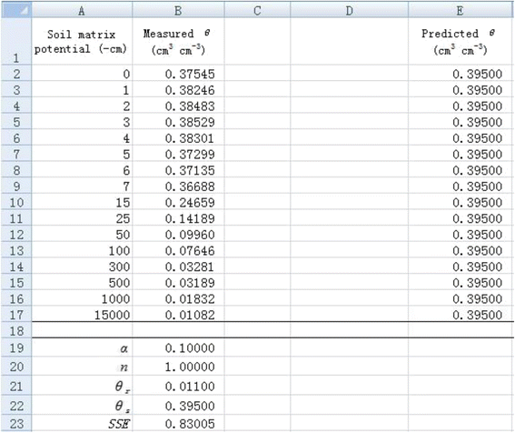
1. List the applied suction pressure as the independent variable in column A and measured soil water content (θ) as the dependent variable in column B (Figure 1).
Data input and initial value set for
α
and
n
in a spreadsheet.
Full size image
2. Temporarily set the value of α as 0.1 and n as 1 in cells B19 and B20, respectively (Figure 1). It is important to set an appropriate initial value because an obviously unreasonable initial value will lead to an unanticipated value. Please refer to related document for initial value estimation (e.g., Delboy 1994). List the measured θ
r
and θ
s
in cells B21 and B22, respectively. Then the predicted θ value can be calculated with the van Genuchten soil water retention curve model (Eq. 5) using suction pressure and all parameter values. For example, the predicted θ in cell E2 (( {widehat{theta}}_{E2} )) is calculated by the following formula:
$$ {widehat{theta}}_{E2}=$B$21+left($B$22-$B$21right)ast left(1+left($B$19ast $A2right)hat{mkern6mu} $B$20right)hat{mkern6mu} left(-1+1/$B$20right) $$
(1)
As Figure 1 shows, all the predicted θ values are 0.395 given the initial values.
3. Calculate the sum of squared residuals (SSE) using Excel function SUMXMY2 in cell B23 by entering “SUMXMY2(B2 : B17, E2 : E17)”. We obtain 0.83005 for SSE for the given initial parameter values (Figure 1).
4. The model obtains the maximum likelihood when the SSE is minimized, which is the principle of least-square fitting method. The Solver tool in Excel can be used to minimize the SSE values. The Solver tool can be found under the Data menu in Excel. If not found there, it has to be added from File menu through the path File- > Options- > Add-Ins- > Solver Add-in. As Figure 2 shows, the “Set Objective” box is the value to be optimized, which is the SSE value in cell B23. Click “Min” to minimize the objective SSE by changing the values of α and n as shown in the “By Changing Variable Cells”.
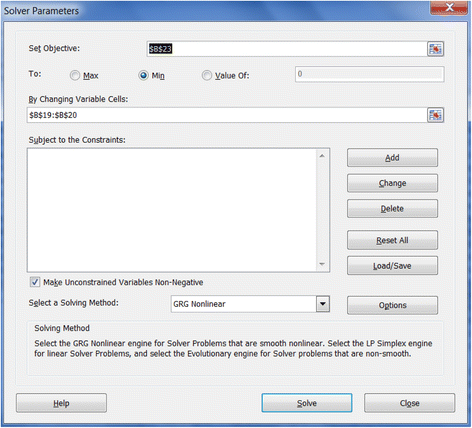
Solver working screen in Excel 2010.
Full size image
5. The Solver will then find the minimum SSE (in cell B23) and corresponding α (in cell B19) and n (in cell B20) values (Figure 3). The measured θ values are in agreement with the predicted θ values (Figure 4), indicating a good nonlinear curve fitting.
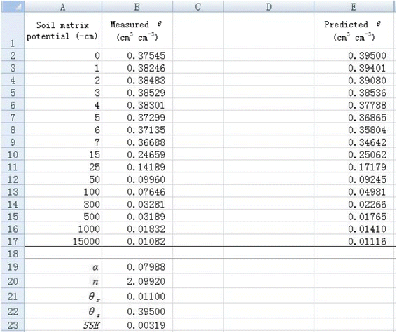
A spreadsheet for estimating nonlinear regression coefficients
α
and
n
.
Full size image
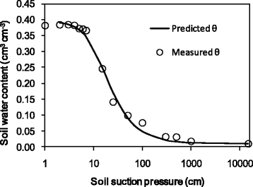
Measured and predicted soil water content versus soil suction pressure.
Full size image
Using Monte Carlo method to estimate parameter uncertainty
Stepwise application of the Monte Carlo method in estimating parameter uncertainties with 200 simulations is demonstrated below:
1. Resample θ using the Monte Carlo method in different columns. Take cell L2 for example, the simulated θ (θ
L2
) is calculated by the following formula:
$$ {theta}_{L2}=$mathrm{E}2+mathrm{NORM}.mathrm{I}mathrm{N}mathrm{V}left(mathrm{RAND}left(right),0,mathrm{SQRT}left(SSE/dfright)right) $$
(2)
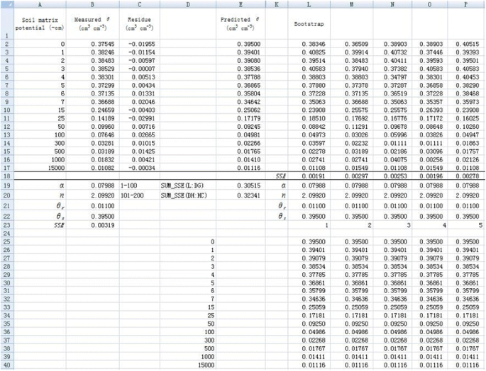
where $E2 refers to the corresponding predicted θ. SSE is the value calculated above, which is the value in cell B23 in Figure 5. The degree of freedom (df) equals 14. The θ values in the other rows in column L are simulated in a similar way. The simulated values for a new dependent variable θ are demonstrated in cells L2-L17 (Figure 5). The same Monte Carlo simulations are performed from column M to column HC. Therefore, a total of 200 sets of simulated θ are obtained (Figure 5).
Resampling dependent variable
θ
using Monte Carlo method and initial values set (only the first 5 simulations are shown).
Full size image
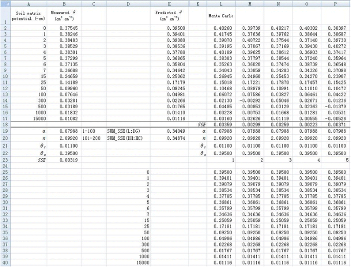
2. Use the same procedure as introduced before to conduct nonlinear regression for each new data set of θ. Note that the new data set of θ will change during optimization, which will result in errors in fitting. Therefore, we copy the simulated θ data to a new sheet by right-clicking “Paste Special” and selecting “Values” in the dialogue of “Paste Special”. For better display, predicted θ array, all the parameter values, and corresponding SSE value are presented in the same column for each simulation (Figure 5). Optimization of parameters α and n is made independently for each simulation using the Solver tool. The initial values are set as the fitted values obtained before for all simulations to reduce the time required during the optimization. Therefore, initial values of 0.07988 and 2.09920 are set for α and n, respectively (Figure 5). Because the maximum number of variables Solver can solve is 200, we can minimize the SSE values for 100 simulations at one time by minimizing the sum of SSE values of 100 simulations. For example, the parameters α and n for the first 100 simulations can be optimized by minimizing cell E19 by entering “=SUM(L18:DG18)” (Figure 5). Similarly, the parameters for the second 100 simulations can be optimized in cell E20 by entering “=SUM(DH18:HC18)”. Therefore, we obtain 200 values for both parameters (α and n) as shown in cells from L19 to HC20 (Figure 6). The frequency distribution of α and n are shown in Figure 7. Visually, both of them follow a normal distribution. However, the Shapiro-Wilk test shows that the parameter α does not conform to a normal distribution, whereas parameter n does. This indicates that the fitted parameters may not necessarily be normally distributed even if the dependent variable is normally distributed, due to the nonlinear relations between them.
Nonlinear regression fitting for resampled
θ
using Monte Carlo method (only the first 5 simulations are shown).
Full size image
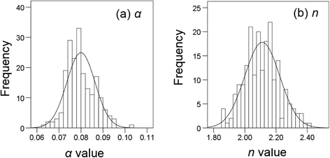
Frequency distribution of (a)
α
and (b)
n
obtained using Monte Carlo method with 200 simulations. The heights of bars indicate the number of parameter values in the equally spaced bins. The curve is the theoretical normal distribution.
Full size image
3. Calculate the 95% confidence interval of α or n values with 200 simulations. We copy all the fitted α or n values, then paste them to a new sheet by right-clicking “Paste Special” and selecting “Transpose” in the dialogue of “Paste Special” to list all the fitted α or n values in one column. Select the transposed data, and rank them in an ascending order using Sort tool in Data tab. Find the value of α and n corresponding to the 2.5 percentile and 97.5 percentile, which are the lower limit and upper limit, respectively, at a 95% confidence. The 95% confidence interval are (0.0680, 0.0939) and (1.9185, 2.3689) for α and n, respectively (Table 1). The difference between upper limit and lower limit is 0.0259 and 0.4504 for α and n, respectively.
Comparison of parameter uncertainties calculated by different methods
Full size table
Using bootstrap method to estimate parameter uncertainty
Stepwise application of the bootstrap method in estimating parameter uncertainties with 200 simulations is demonstrated as follows:
1. Resample θ using the bootstrap method in different columns (Figure 8). Take cell L2 for example, the simulated θ (θ
L2
) can be calculated by the following formula:
Resampling dependent variable
θ
using bootstrap method and initial values set (only the first 5 simulations are shown).
Full size image
$$ {theta}_{L2}=$mathrm{E}2+mathrm{INDEX}left($mathrm{C}:$mathrm{C},mathrm{I}mathrm{N}mathrm{T}left(mathrm{RAND}left(right)*16+2right)right) $$
(3)
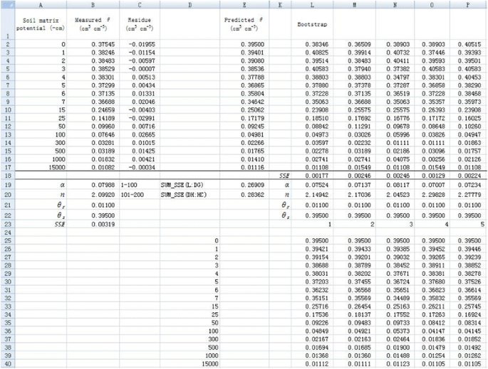
where the function INDEX is used to randomly select a residue value from row 2 to row 17 in column C (the residual is calculated by subtracting predicted θ from the original θ). The θ values at other rows in column L and in other columns (column M to column HC) are simulated in a similar way. Here, 2 in the right hand side of Eq. (3) means that data start at second row.
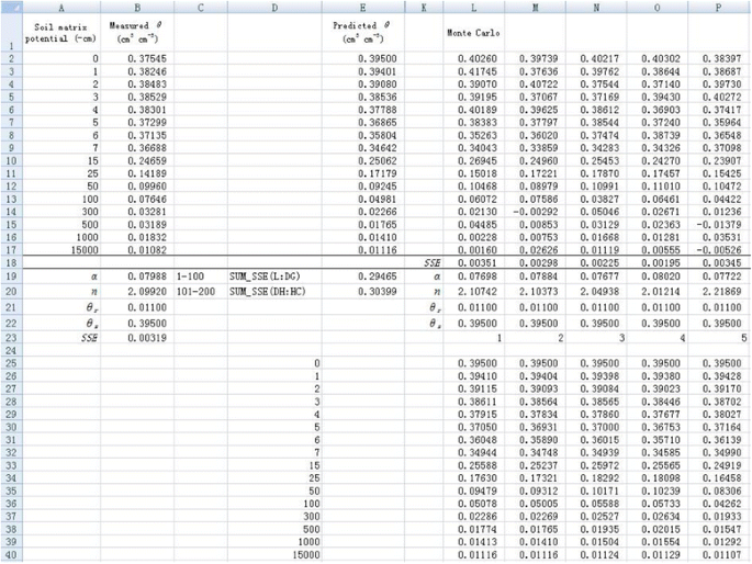
2. Similar to the Monte Carlo method, parameters α and n for all simulations are fitted by minimizing the sum of every 100 SSE values using the Solver tool (Figures 8 and 9). Therefore, we can also obtain 200 values for both parameters (α and n) as shown in cells from L19 to HC20 (Figure 9). The frequency distribution of α and n are shown in Figure 10. They also visually follow a normal distribution. However, the Shapiro-Wilk test shows that the parameter α does not conform to normal distribution, whereas parameter n does.
Nonlinear regression fitting for resampled
θ
using bootstrap method (only the first 5 simulations are shown).
Full size image

Frequency distribution of (a)
α
and (b)
n
obtained using bootstrap method with 200 simulations. The heights of bars indicate the number of parameter values in the equally spaced bins. The curve is the theoretical normal distribution.
Full size image
3. Similar to the Monte Carlo method, the 95% confidence intervals for these two parameters are calculated. They are (0.0680, 0.0925) and (1.9172, 2.3356), for α and n respectively (Table 1). The corresponding difference between upper limit and lower limit is 0.0245 and 0.4183 for α and n, respectively.
Influences of number of simulation on parameter uncertainty analysis
Datasets of fitted values with different numbers of simulations are obtained using a similar method as demonstrated before (data not shown). According to Shapiro-Wilk test, both parameters do not follow a normal distribution with different numbers of simulations except for a few cases that the number of simulations ≤400. This may indicate that the assumption of normality in the linearization method does not hold true.
The lower limit, upper limit, and their difference change slightly with the number of simulations. However, they are almost constant beyond a certain number of simulations (Figure 11). Here, we determine the number of simulations required for both methods according to the change in difference between the upper limit and lower limit. If the relative difference (RD%) of the difference between the upper limit and lower limit under a certain number of simulation is less than 5% compared with that under 2000 simulations, the number of simulations tested is taken to be the required number of simulations. The RD% can be calculated as
$$ mathrm{R}mathrm{D}%=left|frac{{mathrm{V}}_m-{mathrm{V}}_{2000}}{{mathrm{V}}_{2000}}right|*100% $$
(4)
where Vm and V2000 are the differences between the upper limit and lower limit under m simulations and 2000 simulations, respectively.
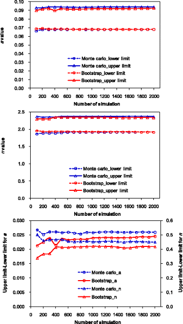
Influences of number of simulation on the lower limit, upper limit, and difference of upper limit and lower limit.
Full size image
For the Monte Carlo method, the RD% is less than 5% for α and n when the numbers of simulation are ≥100 and 200, respectively. For the bootstrap method, the RD% is less than 5% for α and n when the numbers of simulation are ≥500 and 400, respectively. Therefore, simulation number of 200 and 500 are needed to produce reliable data at the 95% confidence interval of parameters for the Monte Carlo and bootstrap methods, respectively. In this sense, the Monte Carlo method may be better than the bootstrap method. However, the optimal number of simulation may also differ with specific situations. For example, Efron and Tibshirani (1993) stated that a minimum of approximately 1000 bootstrap re-samples was sufficient to obtain accurate confidence interval estimates. In order to obtain reliable confidence interval estimates, we suggest increasing the simulation times by 100 at each step, and the final results can be obtained when the values stabilize within consecutive steps.
Comparison with parameter uncertainty approximated by linear model
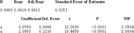
The values α and n are estimated to be 0.0799 and 2.0988, respectively, by SigmaPlot 10.0 (Figure 12), which are exactly the same as the estimates made by nonlinear regression in Excel. Based on the linear model, the associated standard errors are estimated to be 0.0066 and 0.1138, respectively (Figure 12). Then the 95% confidence intervals of α and n are (0.0670, 0.0928) and (1.8758, 2.3218), respectively. As Table 1 shows, the difference between upper limit and lower limit by the Monte Carlo and bootstrap methods are comparable, although the Monte Carlo method produces a slightly greater uncertainty than the bootstrap method. The slight difference is due to the differences in re-sampling residues. While the Monte Carlo simulation generates residues based on a theoretical normal distribution, the bootstrap method randomly takes the residues with replacement and no assumption is made about the underlying distributions. They are also comparable to those approximated by the linear model obtained from the SigmaPlot software. However, by comparing the results of these three methods, the lower limit and upper limit of α and n obtained by the Monte Carlo and bootstrap methods are slightly greater than those obtained based on a linear assumption except for upper limit of α by the bootstrap method. Because the linearization method is based on the assumption of normal distribution of parameters and linearity at the vicinity of the estimated parameter value, and it is more complicated in terms of calculation, the Monte Carlo and bootstrap methods may be preferred to the linearization method to calculate the parameter uncertainties in spreadsheets. Furthermore, the Monte Carlo method may be preferred to the bootstrap method considering the less number of simulations required for the Monte Carlo method. However, if the number of measurements is too small to determine the probability distribution for Monte Carlo method, the bootstrap method may be superior.
Estimates of parameters (
α
and
n
) and associated standard errors using SigmaPlot 10.0.
Full size image
Conclusions
This paper shows step-by-step how to use a Microsoft Excel spreadsheet to fit nonlinear parameters and to estimate their uncertainties using the Monte Carlo and bootstrap methods. Both Monte Carlo and bootstrap methods can be applied in Excel spreadsheets to resample a large number of measurements for dependent variable from which different values of parameters can be obtained. Our results clearly show that the Monte Carlo and bootstrap methods can be used to estimate the parameter uncertainties using spreadsheet methods. The main limitation is that one execution of standard Microsoft Excel Solver has a limit of 200 simultaneous optimizations. This limit can be overcome by multiple independent executions of Solver. Due to the wide accessibility of Microsoft Excel software and ease of use for these two methods, employing the Monte Carlo and bootstrap methods in spreadsheets is strongly recommended to estimate nonlinear regression parameter uncertainties.
In this paper, we demonstrated the methodology with the van Genuchten water retention curve. The method can be applied to any mathematical functions or models that can be evaluated by Excel. Therefore, the methodology presented in this paper has wide applicability. Further, with little modification, the Monte Carlo method or bootstrap method can be used in Microsoft Excel to estimate the uncertainty of hydrologic or environmental predictions with single or multiple input parameters under different degrees of uncertainty.
Methods
Soil water retention curve
Soil water content is a function of soil matric potential ψ under equilibrium conditions, and this relationship θ(ψ) can be described by different types of water retention curves. The soil water retention curve is a basic soil property and is critical for predicting water related environmental processes (Fredlund et al. 1994). Among various soil water retention curve models, the van Genuchten (1980) model is the most widely used one (Han et al. 2010). It is highly nonlinear and can be expressed as:
$$ theta left(uppsi right)={theta}_r+left({theta}_s-{theta}_rright){left(1+{left(alpha left|uppsi right|right)}^nright)}^{-1+frac{1}{n}} $$
(5)
where θ(ψ) is the soil water content [cm3 cm−3] at soil water potential ψ (−cm of water), θ
r
is the residual water content [cm3 cm−3], θ
s
is the saturated water content [cm3 cm−3], α is related to the inverse of the air entry suction [cm−1], and n is a measure of the pore-size distribution (dimensionless). We measured θ(ψ) at 16 soil water potentials for a sandy soil using Tempe pressure cells (at soil matrix potentials ranging from 0 to −500 cm) and pressure plates (at soil water potentials of −1000 and −15000 cm). θ
s
is measured using oven drying method after saturation, and θ
r
is estimated as water content of soil approaching air-dry conditions (Wang et al. 2002). θ
s
and θ
r
are 0.395 and 0.011, respectively. Note that the soil water content (0.375) at zero matrix potential is lower than θ
s
due to the soil water movement under gravity. This paper will focus on the estimation of parameters α and n and their associated 95% confidence intervals.
Parameter uncertainty estimation by linearization of nonlinear model
We express the van Genuchten model (Eq. 5) as:
$$ {theta}_i=fleft(beta, {uppsi}_iright)+{varepsilon}_i $$
(6)
where θ
i
is the i th observation for the dependent variable θ(ψ) (i = 1, 2, …16), ψ
i
is the i th observation for the predictor |ψ|. β is a vector of parameters which includes parameters α and n. ε
i
is a random error, which is assumed to be independent of the errors of other observations and normally distributed with a mean of zero and variance of σ
2.
The sum of squared residuals (SSE) for nonlinear regression can be written as:
$$ SSEleft(beta right)={displaystyle sum }{left({theta}_i-fleft(beta, {uppsi}_iright)right)}^2 $$
(7)
The model has the maximum likelihood when the SSE is minimized. Namely, when the partial derivative
$$ frac{partial SSEleft(beta right)}{partial beta }=-2{displaystyle sum}left({theta}_i-fleft(beta, {uppsi}_iright)right)frac{partial fleft(beta, {uppsi}_iright)}{partial beta } $$
(8)
is zero, parameters β are optimized. Once the optimum values of β are obtained, the parameter uncertainties can be estimated by linearizing the nonlinear model function at the optimum point using the first-order Taylor series expansion method (Fox and Weisberg 2010).
Let
$$ {boldsymbol{F}}_{boldsymbol{ij}}=frac{partial fleft(widehat{beta},{uppsi}_iright)}{partial {beta}_j} $$
(9)
where ( widehat{beta} ) is the optimized value, j refers to the jth of parameters (j = 1, 2, and β
1 = α, β
2 = n).
Assume matrix F = [F
ij
]. In our case,
$$ boldsymbol{F}=left[begin{array}{cc}hfill frac{partial fleft(widehat{beta},{psi}_1right)}{partial alpha}hfill & hfill frac{partial fleft(widehat{beta},{psi}_1right)}{partial n}hfill \ {}hfill frac{partial fleft(widehat{beta},{psi}_2right)}{partial alpha}hfill & hfill frac{partial fleft(widehat{beta},{psi}_2right)}{partial n}hfill \ {}hfill vdots hfill & hfill vdots hfill \ {}hfill frac{partial fleft(widehat{beta},{psi}_{16}right)}{partial alpha}hfill & hfill frac{partial fleft(widehat{beta},{psi}_{16}right)}{partial n}hfill end{array}right] $$
(10)
where ( frac{partial fleft(widehat{beta},{uppsi}_iright)}{partial alpha } ) and ( frac{partial fleft(widehat{beta},{uppsi}_iright)}{partial n} ) can be calculated by the following formulae:
$$ frac{partial fleft(widehat{beta},{psi}_iright)}{partial alpha }=left(fleft(left(widehat{alpha}+varDelta widehat{alpha}right),widehat{n},{psi}_iright)-fleft(left(widehat{alpha}-varDelta widehat{alpha}right),widehat{n},{psi}_iright)right)/left(2varDelta widehat{alpha}right) $$
(11)
$$ frac{partial fleft(widehat{beta},{psi}_iright)}{partial n}=left(fleft(widehat{alpha},left(widehat{n}+varDelta widehat{n}right),{psi}_iright)-fleft(widehat{alpha},left(widehat{n}-varDelta widehat{n}right),{psi}_iright)right)/left(2varDelta widehat{n}right) $$
(12)
where Δ = 0.015, ( widehat{alpha} ) and ( widehat{n} ) are optimized value of α and n, respectively.
The estimated asymptotic covariance matrix (V) of the estimated parameters can be obtained by (Fox and Weisberg 2010):
$$ V=left[begin{array}{cc}hfill {delta}_{alpha alpha}^2hfill & hfill {delta}_{alpha n}^2hfill \ {}hfill {delta}_{nalpha}^2hfill & hfill {delta}_{nn}^2hfill end{array}right]={sigma}^2{left({boldsymbol{F}}^{boldsymbol{hbox{‘}}}boldsymbol{F}right)}^{-1} $$
(13)
where (F
′
F)− 1 is the inverse of F
′
F, and F
′ is a transpose of F.
The σ
2 can be approximated by dividing the SSE by the degree of freedom, df, as in the form (Brown 2001):
$$ {sigma}^2=frac{SSE}{df} $$
(14)
where df is calculated as the number of observations in the sample minus the number of parameters. In this study, df equals 14 (i.e., 16 minus 2).
Therefore, ( {delta}_{alpha alpha}^2 ), ( {delta}_{nn}^2 ), ( {delta}_{alpha n}^2 ) ( or ( {delta}_{nalpha}^2 )) in Eq. (13) are the estimated variance of α, variance of n, and covariance of α and n, respectively. Specifically, δ
αα
and δ
nn
are the standard errors used to characterize the uncertainties of α and n, respectively. At 95% confidence, the intervals of α and n are ( widehat{alpha} ) ±1.96 δ
αα
, ( widehat{n} ) ±1.96 δ
nn
, respectively. SigmaPlot 10.0 is used to estimate the parameters and associated standard errors.
Monte Carlo method to estimate parameter uncertainty
Monte Carlo method is an analytical technique for solving a problem by performing a large number of simulations and inferring a solution from the collective results of the simulations. It is a method to calculate the probability distribution of possible outcomes.
In this paper, Monte Carlo simulation is performed to obtain residues of dependent variable θ. The residues follow a specified distribution with a mean of zero and standard deviation of ( sqrt{SSE/df} ). The simulated residues are added to the predicted θ (( widehat{theta} )) to reconstruct new observations for dependent variable θ. The expression for obtaining new observations for dependent variable θ in Excel is:
$$ theta =widehat{theta}+mathrm{NORM}.mathrm{I}mathrm{N}mathrm{V}left(mathrm{RAND}left(right),0,mathrm{SQRT}left(frac{SSE}{df}right)right) $$
(15)
where function NORM.INV gives a value which follow a normal distribution with a mean of zero and standard deviation of ( sqrt{SSE/df} ) at a probability of RAND(). Therefore, normal distribution on the θ is assumed for Monte Carlo method. Excel function RAND produces a random value that is greater than or equal to 0 and less than 1. SQRT is a function to obtain the square root of a variable.
Monte Carlo simulations are performed 2000 times. Nonlinear regression is made on the simulated θ values versus |ψ| to obtain 2000 values for parameters α and n. The fitted values with different numbers (from 100 to 2000 with intervals of 100) of simulation is analyzed separately to determine the influences of number of simulation on uncertainty estimates. For each dataset, the probability distribution of α and n will be determined by the Shapiro-Wilk test using SPSS 16.0, and the 95% confidence intervals of α and n will be calculated to represent their uncertainties. For simplification, only 200 simulations are shown as an example. Readers can run different numbers of simulation by analogy.
Bootstrap method to estimate parameter uncertainty
Bootstrap method is an alternative method first introduced by Efron (1979) for determining uncertainty in any statistic caused by sampling error. The main idea of this method is to resample with replacement from the sample data at hand and create a large number of “phantom samples” known as bootstrap samples (Singh and Xie 2013). Bootstrap method is a nonparametric method which requires no assumptions about the data distribution.
Residues of θ are calculated by subtracting the ( widehat{theta} ) from the original θ measurements. Bootstrap method is used to resample the residues with replacement for each θ from the calculated residues. The re-sampled residues are added to the ( widehat{theta} ) to reconstruct new observations for dependent variable θ. The expression for obtaining new observations for dependent variable θ using bootstrap method in Excel is:
$$ theta =widehat{theta}+mathrm{INDEX}Big(mathrm{Range} mathrm{of} mathrm{residual},mathrm{I}mathrm{N}mathrm{T}left(mathrm{RAND}left(right)*mathrm{Row} mathrm{number}right) $$
(16)
where function INDEX is used to randomly return a calculated residual from a certain array. Range of residual refers to the calculated residues. INT is a function to round a given number, which is randomly produced by RAND() multiplied by row number.
The non-parametric bootstrap method is a special case of Monte Carlo method used for obtaining the distribution of residues of θ which can be representative of the population. The idea behind the bootstrap method is that the calculated residues can be an estimate of the population, so the distribution of the residues can be obtained by drawing many samples with replacement from the calculated residues. For the Monte Carlo method, however, it creates the distribution of residues of θ with a theoretical (i.e., normal) distribution. From this aspect, the bootstrap method is more empirically based and the Monte Carlo method is more theoretically based.
Similar to the Monte Carlo method, bootstrap simulations are performed 2000 times. Distribution type and 95% confidence intervals of α and n will also be determined for fitted datasets with different numbers (from 100 to 2000 with intervals of 100) of simulation. For simplification, only 200 simulations are shown as an example.
References
-
Berger RL (2007) Nonstandard operator precedence in Excel. Comput Stat Data An 51:2788–2791
Article
Google Scholar
-
Brown AM (2001) A step-by-step guide to non-linear regression analysis of experimental data using a Microsoft Excel spreadsheet. Comp Meth Prog Bio 65:191–200
Article
Google Scholar
-
Conedera M, Torriani D, Neff C, Ricotta C, Bajocco S, Pezzatti GB (2011) Using Monte Carlo simulations to estimate relative fire ignition danger in a low-to-medium fire-prone region. Forest Ecol Manag 26:2179–2187
Article
Google Scholar
-
Cwiertny DM, Roberts AL (2005) On the nonlinear relationship between k(obs) and reductant mass loading in iron batch systems. Environ Sci Technol 39:8948–8957
Article
Google Scholar
-
Delboy H (1994) A non-linear fitting program in pharmacokinetics with Microsoft® Excel spreadsheet. Int J Biomed Comput 37:1–14
Article
Google Scholar
-
Efron B (1979) Bootstrap method: another look at the Jackknife. Ann Stat 7:1–26
Article
Google Scholar
-
Efron B, Tibshirani R (1993) An introduction to the Bootstrap. Champman & Hall, London, UK
Book
Google Scholar
-
Fox J, Weisberg S (2010) Nonlinear regression and nonlinear least squares in R: An appendix to an R companion to applied regression, second edition. http://socserv.socsci.mcmaster.ca/jfox/Books/Companion/appendix/Appendix-Nonlinear-Regression.pdf.
-
Fredlund DG, Xing AQ, Huang SY (1994) Predicting the permeability function for unsaturated soils using the soil-water characteristic curve. Can Geotech J 31:533–546
Article
Google Scholar
-
Han XW, Shao MA, Hortaon R (2010) Estimating van Genuchten model parameters of undisturbed soils using an integral method. Pedosphere 20:55–62
Article
Google Scholar
-
Harris DC (1998) Nonlinear least-squares curve fitting with Microsoft Excel Solver. J Chem Educ 75:119–121
Article
Google Scholar
-
Luo B, Maqsood I, Yin YY, Huang GH, Cohen SJ (2003) Adaption to climate change through water trading under uncertainty — An inexact two-stage nonlinear programming approach. J Environ Inform 2:58–68
Article
Google Scholar
-
Singh K, Xie M (2013) Bootstrap: A statistical method. From Rutgers University. http://www.stat.rutgers.edu/home/mxie/rcpapers/bootstrap.pdf.
-
Smith LH, McCarty PL, Kitanidis PK (1998) Spreadsheet method for evaluation of biochemical reaction rate coefficients and their uncertainties by weighted nonlinear least-squares analysis of the integrated Monod equation. Appl Environ Microbiol 64:2044–2050
Google Scholar
-
Tong L, Chang C, Jin S, Saminathan R (2012) Quantifying uncertainty of emission estimates in National Greenhouse Gas Inventories using bootstrap confidence intervals. Atmos Environ 56:80–87
Article
Google Scholar
-
van Genuchten MT (1980) A closed-form equation for predicting the hydraulic conductivity of unsaturated soils. Soil Sci Soc Am J 44:892–898
Article
Google Scholar
-
Wang QJ, Horton R, Shao MA (2002) Horizontal infiltration method for determining Brooks-Corey model parameters. Soil Sci Soc Am J 66:1733–1739
Article
Google Scholar
-
Wraith JM, Or D (1998) Nonlinear parameter estimation using spreadsheet software. J Nat Resour Life Sci Educ 27:13–19
Google Scholar
Download references
Acknowledgements
The project was funded by the Natural Sciences and Engineering Research Council (NSERC) of Canada.
Author information
Authors and Affiliations
-
Department of Soil Science, University of Saskatchewan, Saskatoon, SK, S7N 5A8, Canada
Wei Hu, Jing Xie & Bing Cheng Si
-
Department of Soil and Physical Science, Lincoln University, PO Box 84, Lincoln, Christchurch, 7647, New Zealand
Henry Wai Chau
Authors
- Wei Hu
You can also search for this author in
PubMed Google Scholar - Jing Xie
You can also search for this author in
PubMed Google Scholar - Henry Wai Chau
You can also search for this author in
PubMed Google Scholar - Bing Cheng Si
You can also search for this author in
PubMed Google Scholar
Corresponding author
Correspondence to
Bing Cheng Si.
Additional information
Competing interests
The author declares that there are no competing interests associated with this research work.
Authors’ contributions
WH analyzed the data and wrote the draft. JX and HC participated in the data analysis. BS designed the study. All authors read and approved the final manuscript.
Authors’ information
Wei Hu is a professional research associate at the University of Saskatchewan and specialist for soil hydrology. Jing Xie is a PhD student in University of Saskatchewan who is investigating legume fertilization. Henry Wai Chau is a lecturer in environmental physics in Lincoln University. Bing Cheng Si is a full professor in University of Saskatchewan and specializes in soil physics.
Rights and permissions
Open Access This article is licensed under a Creative Commons Attribution 4.0 International License, which permits use, sharing, adaptation, distribution and reproduction in any medium or format, as long as you give appropriate credit to the original author(s) and the source, provide a link to the Creative Commons licence, and indicate if changes were made.
The images or other third party material in this article are included in the article’s Creative Commons licence, unless indicated otherwise in a credit line to the material. If material is not included in the article’s Creative Commons licence and your intended use is not permitted by statutory regulation or exceeds the permitted use, you will need to obtain permission directly from the copyright holder.
To view a copy of this licence, visit https://creativecommons.org/licenses/by/4.0/.
Reprints and Permissions
About this article
Cite this article
Hu, W., Xie, J., Chau, H.W. et al. Evaluation of parameter uncertainties in nonlinear regression using Microsoft Excel Spreadsheet.
Environ Syst Res 4, 4 (2015). https://doi.org/10.1186/s40068-015-0031-4
Download citation
-
Received: 22 January 2015
-
Accepted: 11 March 2015
-
Published: 24 March 2015
-
DOI: https://doi.org/10.1186/s40068-015-0031-4
Keywords
- Bootstrap
- Monte Carlo
- Soil water retention
- Parameter uncertainty
- Excel
На чтение 5 мин Просмотров 2.4к. Опубликовано 03.07.2021
Содержание
- Материал из MachineLearning.
- Содержание
- Описание критерия
- Критерий Шапиро-Франчиа
- Решение «табличной проблемы»
- Электронные таблицы
- Правила пользования таблицами
Материал из MachineLearning.
Содержание
Критерий Шапиро-Уилка используется для проверки гипотезы : «случайная величина распределена нормально» и является одним наиболее эффективных критериев проверки нормальности. Критерии, проверяющие нормальность выборки, являются частным случаем критериев согласия. Если выборка нормальна, можно далее применять мощные параметрические критерии, например, критерий Фишера.
Описание критерия
Критерий Шапиро-Уилка основан на оптимальной линейной несмещённой оценке дисперсии к её обычной оценке методом максимального правдоподобия. Статистика критерия имеет вид:
Числитель является квадратом оценки среднеквадратического отклонения Ллойда.
Коэффициенты берутся из таблиц. Ниже приведена таблица для небольших значений n и i.
| n | i | |||||||||
|---|---|---|---|---|---|---|---|---|---|---|
| 1 | 2 | 3 | 4 | 5 | 6 | 7 | 8 | 9 | 10 | |
| 3 | 7071 | |||||||||
| 4 | 6872 | 1677 | ||||||||
| 5 | 6646 | 2413 | ||||||||
| 6 | 6431 | 2806 | 0875 | |||||||
| 7 | 6233 | 3031 | 1401 | |||||||
| 8 | 6052 | 3164 | 1743 | 0561 | ||||||
| 9 | 5888 | 3244 | 1976 | 0947 | ||||||
| 10 | 5739 | 3291 | 2141 | 1224 | 0399 | |||||
| 11 | 5601 | 3315 | 2260 | 1429 | 0695 | |||||
| 12 | 5475 | 3325 | 2347 | 1586 | 0922 | 0303 | ||||
| 13 | 5359 | 3325 | 2412 | 1707 | 1099 | 0539 | ||||
| 14 | 5251 | 3318 | 2460 | 1802 | 1240 | 0727 | 0240 | |||
| 15 | 5150 | 3306 | 2495 | 1878 | 1353 | 0880 | 0433 | |||
| 16 | 5056 | 3290 | 2521 | 1939 | 1447 | 1005 | 0593 | 0196 | ||
| 17 | 4968 | 3237 | 2540 | 1988 | 1524 | 1109 | 0725 | 0359 | ||
| 18 | 4886 | 3253 | 2553 | 2027 | 1587 | 1197 | 0837 | 0496 | 0173 | |
| 19 | 4808 | 3232 | 2561 | 2059 | 1641 | 1271 | 0932 | 0612 | 0303 | |
| 20 | 4734 | 3211 | 2565 | 2085 | 1686 | 1334 | 1013 | 0711 | 0422 | 0140 |
| 21 | 4634 | 3185 | 2578 | 2119 | 1736 | 1399 | 1092 | 0804 | 0530 | 0263 |
Критические значения статистики также находятся таблично.
Если , то нулевая гипотеза о нормальности распределения отклоняется при уровне значимости Приближённая вероятность получения эмпирического значения при вычисляется по формуле
где — табличные коэффициенты.
Критерий Шапиро-Уилка является очень мощным критерием для проверки нормальности, но, к сожалению, имеет ограниченную применимость. При больших значениях 100)» alt= «n ;(n>100)» /> таблицы коэффициентов становятся неудобными. Поэтому была предложена модификация критерия Шапиро-Уилка, о которой рассказано ниже.
Критерий Шапиро-Франчиа
Введённая статистика имеет вид
где и — математическое ожидание i-й порядковой статистики стандартного нормального распределения. Аппроксимация где не искажает существенно критерий
Используя аппрокисмацию для квантили стандартного нормального распределения, можно записать
Решение «табличной проблемы»
Была выведена полезная аппрокисмация, позволяющая применить критерий Шапиро-Уилка без помощи таблиц. Для предлагается статистика
Если то нулевая гипотеза нормальности распределения случайных величин отклоняется. Существует модификация критерия Шапиро-Уилка для случаев группированных данных (что существенно при наличии совпадающих наблюдений).
В ряде опытов, особенно в медицинских исследованиях, численность выборки мала. Специально для проверки нормальности распределения малых, численностью от трех до пятидесяти элементов, выборок Шапиро и Уилк разработали критерий .
Итак, пусть имеется выборка . Вычисления статистики производятся по формулам:
где и . Значение в последней формуле определяется следующим образом:
, если — четное, , если — нечетное, — известные константы.
Для вычисления реально достигнутого уровня значимости применяется нормальная аппроксимация, используется следующая формула:
где — стандартное нормальное распределение, , и — константы, для которых известны, в зависимости от объема выборки, табличные значения.
Электронные таблицы
| Результаты вычислений | ||
|---|---|---|
| Объем выборки | Значение статистики Шапиро-Уилка | Достигаемый уровень значимости |
| Реализация исследуемой выборки |
|---|
Правила пользования таблицами
Прежде всего в текстовое поле следует поместить изучаемую выборку (это можно сделать, набрав соответствующие значения вручную либо скопировав, скажем из Excel), затем нажать кнопку «Вычислить», после чего в таблице «Результаты вычислений» появится реально достигнутый уровень значимости в критерии Шапиро-Уилка, а также объем выборки и значение статистики Шапиро-Уилка.
Отметим, что в качестве десятичного разделителя в числах можно использовать и точку, и запятую. Удалять значения из первой таблицы можно двойным щелчком мыши. Особо обратим внимание! В качестве разделителя между отдельными числами ни в коем случае не следует использовать точку и запятую, так как эти знаки используются в качестве десятичного разделителя. Отделить одно число от другого можно используя «пробел» или «ввод». Скажем, такой ввод в текстовое поле верен:
0,23 0,56 0.98
0,98 1,56 9,9 7.908
Соответственно будут обрабатываться семь значений: 0.23 0.56 0.98 1.56 9.9 7.908.
Статистику критерия рассчитывают по формуле W =b 2 /nm2. Рассчитанное значение W сравнивают с табличным Wтабл. Табличные значения критерия Wтабл в зависимости от уровня значимости α находят из таблиц, однако с приемлемой точностью их можно найти по зависимостям, показанным в табл. 9.2.
Таблица 9.2.
| α | Wтабл |
| 0,01 | (-0,0148n 4 + 2,1875n 3 — 122,61n 2 + 3257,3n + 55585)/100000 |
| 0,05 | (-0,0113n 4 + 1,656n 3 — 91,88n 2 + 2408,6n + 67608)/100000 |
| 0,1 | (-0,0084n 4 + 1,2513n 3 — 70,724n 2 + 1890n + 73840)/100000 |
Если W >= Wтабл, нулевую гипотезу не бракуют, т.е. распределение считают нормальным.
Пример 9.1. По данным примера 1.1 проверить при различных уровнях значимости гипотезу о нормальности распределения предела прочности на разрыв алюминиевого сплава.
Вариант выполнения примера 9.1 показан на рисунке 9.1.

Рис. 9.1. Вариант расчёта для примера 9.1.
Вводим в электронную таблицу уровень значимости и результаты испытаний, упорядочиваем их в вариационном ряду, рассчитываем среднее значение, сумму квадратов отклонений от среднего nm2, объём испытаний (какие при этом целесообразно задать в статистических функциях диапазоны?), а также величину k. Очевидно, что для любого (чётного и нечётного) n можно рассчитать k по формуле k=n/2 с округлением результата вниз до целого (функция ОКРУГЛВНИЗ).
Далее находим b. Для этого вначале рассчитываем значения n-i+1. Поскольку при этом, в соответствии с формулой (9.1), i = k, при расчёте используем функцию ЕСЛИ, в которой логическим выражением будет n-i+1>= k (т.е. ссылка на ячейку столбца G). При истинности этого выражения значение xn-i+1 находим при помощи функции ИНДЕКС, при ложности значение не задаём. Затем находим x 2 и W. Рассчитываем табличные значения критерия для различных уровней значимости по формулам табл. 7.2. Из этих значений выбираем необходимое Wтабл в соответствии с заданным уровнем значимости, используя трижды функции ЕСЛИ.
Затем, если n < 8, с помощью функции ЕСЛИ выводим сообщение «ВЫБОРКА СЛИШКОМ МАЛА». При ложности этого логического выражения используем в строке Значение_если_ложь функцию ЕСЛИ для сравнивания W и Wтабл, и в зависимости от истинности или ложности логического выражения выводим сообщение, является ли распределение нормальным. В результате в одной ячейке (в примере – ячейка D18) должно выводиться одно из трёх сообщений, например: ВЫБОРКА СЛИШКОМ МАЛА; РАСПРЕД. НОРМАЛЬНОЕ; РАСПРЕД. НЕ НОРМАЛЬНОЕ.
При правильном выполнении электронная таблица должна вер-но пересчитываться при вводе других данных в пределах применимо-сти критерия Шапиро-Уилка.
Задание.
1. Выполнить расчёты в соответствии с примером 9.1.
2. Выборочные значения случайных величин, полученные по результатам испытаний, показаны в табл. 9.3.
Таблица 9.3.
| № выборки | Р | Значения в выборке |
| 1 | 0,9 | 855 875 834 872 863 855 888 864 870 881 891 872 |
| 2 | 0,95 | 11 12 9 16 12 8 9 10 10 9 11 10 8 8 |
| 3 | 0,99 | 34 36 38 33 34 32 30 36 38 31 |
Предполагается, что случайные величины распределены нормально.. Используя созданные электронные таблицы, исключить грубые ошибки по критерию Ирвина, проверить нормальность распределений, в случае нормального распределения рассчитать интервальные оценки параметров этих распределений. Результаты занести в таблицу 9.4.
Таблица 9.4.
| № выборки | Грубые ошибки | Распределение (норм/не норм) | Оценка М | Оценка σ | ||
| точечная | Интерв. | точечная | Интерв. | |||
| 1 | . | . | . | . | . | . |
| 2 | . | . | . | . | . | . |
| 3 | . | . | . | . | . | . |
        Далее     Содержание
- Распечатать
Оцените статью:
- 5
- 4
- 3
- 2
- 1
(2 голоса, среднее: 1 из 5)
Поделитесь с друзьями!
Тест Шапиро – Уилка — это тест нормальности в частотном статистика. Он был опубликован в 1965 году Сэмюэлем Сэнфордом Шапиро и Мартином Уилком.
Содержание
- 1 Теория
- 2 Интерпретация
- 3 Анализ мощности
- 4 Приближение
- 5 См. Также
- 6 Ссылки
- 7 Внешние ссылки
Теория
Тест Шапиро – Уилка проверяет нулевую гипотезу о том, что образец x1,…, x n произошли от нормально распределенной популяции. Тестовая статистика :
- W = (∑ i = 1 naix (i)) 2 ∑ i = 1 n (xi — x ¯) 2, { displaystyle W = { left ( sum _ {i = 1} ^ {n} a_ {i} x _ {(i)} right) ^ {2} over sum _ {i = 1} ^ {n} (x_ {i} — { overline {x}}) ^ {2}},}


где
Коэффициенты ai { displaystyle a_ {i}} задаются следующим образом:
- (a 1,…, an) = m TV — 1 C, { displaystyle (a_ {1}, dots, a_ {n}) = {m ^ { mathsf {T}} V ^ {- 1} over C},}

где C — вектор норма :
- С = ‖ В — 1 м ‖ = (м ТВ — 1 В — 1 м) 1/2 { displaystyle C = | V ^ {- 1} m | = (m ^ { mathsf { T}} V ^ {- 1} V ^ {- 1} m) ^ {1/2}}

и вектор m,
- m = (m 1,…, mn) T { displaystyle m знак равно m_ {1}, dots, m_ {n}) ^ { mathsf {T}} ,}

состоит из ожидаемых значений из статистики заказа независимые и одинаково распределенные случайные величины, выбранные из стандартного нормального распределения; наконец, V { displaystyle V} — это ковариационная матрица этой статистики нормального порядка.
Нет названия для распределения W { Displaystyle W} . Пороговые значения для статистики вычисляются с помощью моделирования Монте-Карло.
Интерпретация
нулевая гипотеза этого теста заключается в том, что совокупность распределена нормально. Таким образом, если значение p меньше, чем выбранный альфа-уровень, то нулевая гипотеза отклоняется, и есть свидетельства того, что проверенные данные не имеют нормального распределения. С другой стороны, если значение p больше, чем выбранный альфа-уровень, то нулевая гипотеза (что данные пришли из нормально распределенной совокупности) не может быть отклонена (например, для альфа-уровня 0,05 набор данных со значением p менее 0,05 отвергает нулевую гипотезу о том, что данные получены из нормально распределенной совокупности).
Как и большинство тестов статистической значимости, если размер выборки достаточно велик, этот тест может обнаруживать даже тривиальные отклонения от нулевой гипотезы (т. е. хотя может быть некоторый статистически значимый эффект, он может быть слишком мал, чтобы иметь какое-либо практическое значение); таким образом, обычно рекомендуется дополнительное исследование величины эффекта, например, в данном случае график Q – Q.
Анализ мощности
Моделирование Монте-Карло обнаружило, что Шапиро –Уилк имеет наилучшую степень для данного значимости, за ним следует Андерсон – Дарлинг при сравнении Шапиро – Уилка, Колмогорова – Смирнова, тесты Лиллиэфорса и Андерсона – Дарлинга.
Аппроксимация
Ройстон предложил альтернативный метод вычисления вектора коэффициентов, предоставив алгоритм вычисления значений, который расширил выборку размер до 2000. Этот метод используется в нескольких программных пакетах, включая Stata, SPSS и SAS. Рахман и Говидараджулу увеличили размер выборки до 5 000.
См. Также
- Тест Андерсона – Дарлинга
- Критерий Крамера – фон Мизеса
- К-квадрат Д’Агостино
- Колмогоров– Тест Смирнова
- Тест Лиллиефорса
- График нормальной вероятности
- Тест Шапиро – Франсиа
Литература
- ^ Shapiro, SS; Вилк, М.Б. (1965). «Тест дисперсионного анализа на нормальность (полные выборки)». Биометрика. 52(3–4): 591–611. doi : 10.1093 / biomet / 52.3-4.591. JSTOR 2333709. MR 0205384. стр. 593
- ^ [1]
- ^[2]
- ^«Как мне интерпретировать тест Шапиро-Уилка на нормальность?». JMP. 2004. Получено 24 марта 2012 г..
- ^Филд, Энди (2009). Обнаружение статистики с помощью SPSS (3-е изд.). Лос-Анджелес [т.е. Таузенд-Оукс, Калифорния]: SAGE Publications. п. 143. ISBN 978-1-84787-906-6 .
- ^Разали, Норнадия; Вау, Яп Би (2011). «Силовые сравнения тестов Шапиро – Вилка, Колмогорова – Смирнова, Лиллиефорса и Андерсона – Дарлинга». Журнал статистического моделирования и аналитики. 2 (1): 21–33. Проверено 30 марта 2017 г.
- ^Ройстон, Патрик (сентябрь 1992 г.). «Аппроксимация W-критерия Шапиро-Уилка на ненормальность». Статистика и вычисления. 2 (3): 117–119. doi : 10.1007 / BF01891203.
- ^Ройстон, Патрик. «Тесты Шапиро – Вилка и Шапиро – Франсиа». Технический бюллетень Stata, StataCorp LP. 1 (3).
- ^Тесты Шапиро-Уилка и Шапиро-Франсиа на нормальность
- ^Пак, Хун Мён (2002–2008). «Одномерный анализ и проверка нормальности с использованием SAS, Stata и SPSS» (PDF). [рабочий документ]. Проверено 26 февраля 2014 г.
- ^Rahman und Govidarajulu (1997). «Модификация теста Шапиро и Уилка на нормальность». Журнал прикладной статистики. 24 (2): 219–236. doi : 10.1080 / 02664769723828.
Внешние ссылки
- Рабочий пример с использованием Excel
- Алгоритм AS R94 (Шапиро Уилк) Код FORTRAN
- Исследовательский анализ с использованием теста нормальности Шапиро – Уилка в R
- Реальная статистика с использованием Excel: расширенный тест Шапиро-Уилка