
| title | keywords | f1_keywords | ms.prod | api_name | ms.assetid | ms.date | ms.localizationpriority |
|---|---|---|---|---|---|---|---|
|
Range object (Excel) |
vbaxl10.chm143072 |
vbaxl10.chm143072 |
excel |
Excel.Range |
b8207778-0dcc-4570-1234-f130532cc8cd |
08/14/2019 |
high |
Range object (Excel)
Represents a cell, a row, a column, a selection of cells containing one or more contiguous blocks of cells, or a 3D range.
[!includeAdd-ins note]
Remarks
The default member of Range forwards calls without parameters to the Value property and calls with parameters to the Item member. Accordingly, someRange = someOtherRange is equivalent to someRange.Value = someOtherRange.Value, someRange(1) to someRange.Item(1) and someRange(1,1) to someRange.Item(1,1).
The following properties and methods for returning a Range object are described in the Example section:
- Range and Cells properties of the Worksheet object
- Range and Cells properties of the Range object
- Rows and Columns properties of the Worksheet object
- Rows and Columns properties of the Range object
- Offset property of the Range object
- Union method of the Application object
Example
Use Range (arg), where arg names the range, to return a Range object that represents a single cell or a range of cells. The following example places the value of cell A1 in cell A5.
Worksheets("Sheet1").Range("A5").Value = _
    Worksheets("Sheet1").Range("A1").Value
The following example fills the range A1:H8 with random numbers by setting the formula for each cell in the range. When it’s used without an object qualifier (an object to the left of the period), the Range property returns a range on the active sheet. If the active sheet isn’t a worksheet, the method fails.
Use the Activate method of the Worksheet object to activate a worksheet before you use the Range property without an explicit object qualifier.
Worksheets("Sheet1").Activate
Range("A1:H8").Formula = "=Rand()"    'Range is on the active sheet
The following example clears the contents of the range named Criteria.
[!NOTE]
If you use a text argument for the range address, you must specify the address in A1-style notation (you cannot use R1C1-style notation).
Worksheets(1).Range("Criteria").ClearContents
Use Cells on a worksheet to obtain a range consisting all single cells on the worksheet. You can access single cells via Item(row, column), where row is the row index and column is the column index.
Item can be omitted since the call is forwarded to it by the default member of Range.
The following example sets the value of cell A1 to 24 and of cell B1 to 42 on the first sheet of the active workbook.
Worksheets(1).Cells(1, 1).Value = 24
Worksheets(1).Cells.Item(1, 2).Value = 42
The following example sets the formula for cell A2.
ActiveSheet.Cells(2, 1).Formula = "=Sum(B1:B5)"
Although you can also use Range("A1") to return cell A1, there may be times when the Cells property is more convenient because you can use a variable for the row or column. The following example creates column and row headings on Sheet1. Be aware that after the worksheet has been activated, the Cells property can be used without an explicit sheet declaration (it returns a cell on the active sheet).
[!NOTE]
Although you could use Visual Basic string functions to alter A1-style references, it is easier (and better programming practice) to use theCells(1, 1)notation.
Sub SetUpTable()
Worksheets("Sheet1").Activate
For TheYear = 1 To 5
    Cells(1, TheYear + 1).Value = 1990 + TheYear
Next TheYear
For TheQuarter = 1 To 4
    Cells(TheQuarter + 1, 1).Value = "Q" & TheQuarter
Next TheQuarter
End Sub
Use_expression_.Cells, where expression is an expression that returns a Range object, to obtain a range with the same address consisting of single cells.
On such a range, you access single cells via Item(row, column), where are relative to the upper-left corner of the first area of the range.
Item can be omitted since the call is forwarded to it by the default member of Range.
The following example sets the formula for cell C5 and D5 of the first sheet of the active workbook.
Worksheets(1).Range("C5:C10").Cells(1, 1).Formula = "=Rand()"
Worksheets(1).Range("C5:C10").Cells.Item(1, 2).Formula = "=Rand()"
Use Range (cell1, cell2), where cell1 and cell2 are Range objects that specify the start and end cells, to return a Range object. The following example sets the border line style for cells A1:J10.
[!NOTE]
Be aware that the period in front of each occurrence of the Cells property is required if the result of the preceding With statement is to be applied to the Cells property. In this case, it indicates that the cells are on worksheet one (without the period, the Cells property would return cells on the active sheet).
With Worksheets(1)
    .Range(.Cells(1, 1), _
        .Cells(10, 10)).Borders.LineStyle = xlThick
End With
Use Rows on a worksheet to obtain a range consisting all rows on the worksheet. You can access single rows via Item(row), where row is the row index.
Item can be omitted since the call is forwarded to it by the default member of Range.
[!NOTE]
It’s not legal to provide the second parameter of Item for ranges consisting of rows. You first have to convert it to single cells via Cells.
The following example deletes row 5 and 10 of the first sheet of the active workbook.
Worksheets(1).Rows(10).Delete
Worksheets(1).Rows.Item(5).Delete
Use Columns on a worksheet to obtain a range consisting all columns on the worksheet. You can access single columns via Item(row) [sic], where row is the column index given as a number or as an A1-style column address.
Item can be omitted since the call is forwarded to it by the default member of Range.
[!NOTE]
It’s not legal to provide the second parameter of Item for ranges consisting of columns. You first have to convert it to single cells via Cells.
The following example deletes column «B», «C», «E», and «J» of the first sheet of the active workbook.
Worksheets(1).Columns(10).Delete
Worksheets(1).Columns.Item(5).Delete
Worksheets(1).Columns("C").Delete
Worksheets(1).Columns.Item("B").Delete
Use_expression_.Rows, where expression is an expression that returns a Range object, to obtain a range consisting of the rows in the first area of the range.
You can access single rows via Item(row), where row is the relative row index from the top of the first area of the range.
Item can be omitted since the call is forwarded to it by the default member of Range.
[!NOTE]
It’s not legal to provide the second parameter of Item for ranges consisting of rows. You first have to convert it to single cells via Cells.
The following example deletes the ranges C8:D8 and C6:D6 of the first sheet of the active workbook.
Worksheets(1).Range("C5:D10").Rows(4).Delete
Worksheets(1).Range("C5:D10").Rows.Item(2).Delete
Use_expression_.Columns, where expression is an expression that returns a Range object, to obtain a range consisting of the columns in the first area of the range.
You can access single columns via Item(row) [sic], where row is the relative column index from the left of the first area of the range given as a number or as an A1-style column address.
Item can be omitted since the call is forwarded to it by the default member of Range.
[!NOTE]
It’s not legal to provide the second parameter of Item for ranges consisting of columns. You first have to convert it to single cells via Cells.
The following example deletes the ranges L2:L10, G2:G10, F2:F10 and D2:D10 of the first sheet of the active workbook.
Worksheets(1).Range("C5:Z10").Columns(10).Delete
Worksheets(1).Range("C5:Z10").Columns.Item(5).Delete
Worksheets(1).Range("C5:Z10").Columns("D").Delete
Worksheets(1).Range("C5:Z10").Columns.Item("B").Delete
Use Offset (row, column), where row and column are the row and column offsets, to return a range at a specified offset to another range. The following example selects the cell three rows down from and one column to the right of the cell in the upper-left corner of the current selection. You cannot select a cell that is not on the active sheet, so you must first activate the worksheet.
Worksheets("Sheet1").Activate
  'Can't select unless the sheet is active
Selection.Offset(3, 1).Range("A1").Select
Use Union (range1, range2, …) to return multiple-area ranges—that is, ranges composed of two or more contiguous blocks of cells. The following example creates an object defined as the union of ranges A1:B2 and C3:D4, and then selects the defined range.
Dim r1 As Range, r2 As Range, myMultiAreaRange As Range
Worksheets("sheet1").Activate
Set r1 = Range("A1:B2")
Set r2 = Range("C3:D4")
Set myMultiAreaRange = Union(r1, r2)
myMultiAreaRange.Select
If you work with selections that contain more than one area, the Areas property is useful. It divides a multiple-area selection into individual Range objects and then returns the objects as a collection. Use the Count property on the returned collection to verify a selection that contains more than one area, as shown in the following example.
Sub NoMultiAreaSelection()
    NumberOfSelectedAreas = Selection.Areas.Count
    If NumberOfSelectedAreas > 1 Then
        MsgBox "You cannot carry out this command " & _
            "on multi-area selections"
    End If
End Sub
This example uses the AdvancedFilter method of the Range object to create a list of the unique values, and the number of times those unique values occur, in the range of column A.
Sub Create_Unique_List_Count()
    'Excel workbook, the source and target worksheets, and the source and target ranges.
    Dim wbBook As Workbook
    Dim wsSource As Worksheet
    Dim wsTarget As Worksheet
    Dim rnSource As Range
    Dim rnTarget As Range
    Dim rnUnique As Range
    'Variant to hold the unique data
    Dim vaUnique As Variant
    'Number of unique values in the data
    Dim lnCount As Long

    'Initialize the Excel objects
    Set wbBook = ThisWorkbook
    With wbBook
        Set wsSource = .Worksheets("Sheet1")
        Set wsTarget = .Worksheets("Sheet2")
    End With

    'On the source worksheet, set the range to the data stored in column A
    With wsSource
        Set rnSource = .Range(.Range("A1"), .Range("A100").End(xlDown))
    End With

    'On the target worksheet, set the range as column A.
    Set rnTarget = wsTarget.Range("A1")

    'Use AdvancedFilter to copy the data from the source to the target,
    'while filtering for duplicate values.
    rnSource.AdvancedFilter Action:=xlFilterCopy, _
                            CopyToRange:=rnTarget, _
                            Unique:=True

    'On the target worksheet, set the unique range on Column A, excluding the first cell
    '(which will contain the "List" header for the column).
    With wsTarget
        Set rnUnique = .Range(.Range("A2"), .Range("A100").End(xlUp))
    End With

    'Assign all the values of the Unique range into the Unique variant.
    vaUnique = rnUnique.Value

    'Count the number of occurrences of every unique value in the source data,
    'and list it next to its relevant value.
    For lnCount = 1 To UBound(vaUnique)
        rnUnique(lnCount, 1).Offset(0, 1).Value = _
            Application.Evaluate("COUNTIF(" & _
            rnSource.Address(External:=True) & _
            ",""" & rnUnique(lnCount, 1).Text & """)")
    Next lnCount

    'Label the column of occurrences with "Occurrences"
    With rnTarget.Offset(0, 1)
        .Value = "Occurrences"
        .Font.Bold = True
    End With

End Sub
Methods
- Activate
- AddComment
- AddCommentThreaded
- AdvancedFilter
- AllocateChanges
- ApplyNames
- ApplyOutlineStyles
- AutoComplete
- AutoFill
- AutoFilter
- AutoFit
- AutoOutline
- BorderAround
- Calculate
- CalculateRowMajorOrder
- CheckSpelling
- Clear
- ClearComments
- ClearContents
- ClearFormats
- ClearHyperlinks
- ClearNotes
- ClearOutline
- ColumnDifferences
- Consolidate
- ConvertToLinkedDataType
- Copy
- CopyFromRecordset
- CopyPicture
- CreateNames
- Cut
- DataTypeToText
- DataSeries
- Delete
- DialogBox
- Dirty
- DiscardChanges
- EditionOptions
- ExportAsFixedFormat
- FillDown
- FillLeft
- FillRight
- FillUp
- Find
- FindNext
- FindPrevious
- FlashFill
- FunctionWizard
- Group
- Insert
- InsertIndent
- Justify
- ListNames
- Merge
- NavigateArrow
- NoteText
- Parse
- PasteSpecial
- PrintOut
- PrintPreview
- RemoveDuplicates
- RemoveSubtotal
- Replace
- RowDifferences
- Run
- Select
- SetCellDataTypeFromCell
- SetPhonetic
- Show
- ShowCard
- ShowDependents
- ShowErrors
- ShowPrecedents
- Sort
- SortSpecial
- Speak
- SpecialCells
- SubscribeTo
- Subtotal
- Table
- TextToColumns
- Ungroup
- UnMerge
Properties
- AddIndent
- Address
- AddressLocal
- AllowEdit
- Application
- Areas
- Borders
- Cells
- Characters
- Column
- Columns
- ColumnWidth
- Comment
- CommentThreaded
- Count
- CountLarge
- Creator
- CurrentArray
- CurrentRegion
- Dependents
- DirectDependents
- DirectPrecedents
- DisplayFormat
- End
- EntireColumn
- EntireRow
- Errors
- Font
- FormatConditions
- Formula
- FormulaArray
- FormulaHidden
- FormulaLocal
- FormulaR1C1
- FormulaR1C1Local
- HasArray
- HasFormula
- HasRichDataType
- Height
- Hidden
- HorizontalAlignment
- Hyperlinks
- ID
- IndentLevel
- Interior
- Item
- Left
- LinkedDataTypeState
- ListHeaderRows
- ListObject
- LocationInTable
- Locked
- MDX
- MergeArea
- MergeCells
- Name
- Next
- NumberFormat
- NumberFormatLocal
- Offset
- Orientation
- OutlineLevel
- PageBreak
- Parent
- Phonetic
- Phonetics
- PivotCell
- PivotField
- PivotItem
- PivotTable
- Precedents
- PrefixCharacter
- Previous
- QueryTable
- Range
- ReadingOrder
- Resize
- Row
- RowHeight
- Rows
- ServerActions
- ShowDetail
- ShrinkToFit
- SoundNote
- SparklineGroups
- Style
- Summary
- Text
- Top
- UseStandardHeight
- UseStandardWidth
- Validation
- Value
- Value2
- VerticalAlignment
- Width
- Worksheet
- WrapText
- XPath
See also
- Excel Object Model Reference
[!includeSupport and feedback]
Ranges are a key concept in Excel, and knowing how to work with them is essential for anyone who wants to program or automate their work using Excel VBA.
In this tutorial, we’ll take a look at how to work with Excel ranges in VBA. We’ll start by discussing what a Range object is. Then, we’ll look at the different ways of referencing a range. Lastly, we’ll explore various examples of how to work with ranges using VBA code.
Excel VBA: The Range object
The Excel VBA Range object is used to represent a range in a worksheet. A range can be a cell, a group of cells, or even all the 17,179,869,184 cells in a sheet.
When programming with Excel VBA, the Range object is going to be your best friend. That’s because much of your work will focus on manipulating data within sheets. Understanding how to work with the Range object will make it easier for you to perform various actions on cells, such as changing their values, sorting, or doing a copy-paste.
The following is the Excel object hierarchy:
Application > Workbook > Worksheet > Range
You can see that the Excel VBA Range object is a property of the Worksheet object. This means that you can access a range by specifying the name of the sheet and the cell address you want to work with. When you don’t specify a sheet name, by default Excel will look for the range in the active sheet. For example, if Sheet1 is active, then both of these lines will refer to the same cell range:
Range("A1")
Worksheets("Sheet1").Range("A1")
Let’s have a closer look at how to reference a range in the section below.


Referencing a range of cells in Excel VBA
Referring to a Range object in Excel VBA can be done in several ways. We’ll discuss the basic syntax and some alternatives that you might want to use, depending on your needs.
Excel VBA: Syntax for specifying a cell range
To refer to a range that consists of one cell, for example, cell D5, you can use the syntax below:
Range("D5")
To refer to a range of cells, you have two acceptable syntaxes. For example, A1 through D5 can be specified using any one below:
Range("A1:D5")
Range("A1", "D5")
To refer to a range outside the active sheet, you need to include the worksheet name. Here’s an example:
Worksheets("Sheet1").Range("A1:D5")
To refer to an entire row, for example, Row 5:
Range("5:5")
To refer to an entire column, for example, Column D:
Range("D:D")
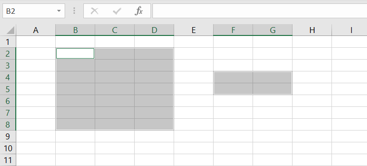
Excel VBA also allows you to refer to multiple ranges at once by using a comma to separate each area. For example, see the below syntax used for referring to all ranges shown in the image:
Range("B2:D8, F4:G5")
Tip: Notice that all of the syntaxes above use double quotes to enclose the range address. To make it quicker for you to type, you can use shortcuts that involve using square brackets without quotes, as shown in the table below:
| Syntax | Shortcut |
|---|---|
Range("D5") |
[D5] |
Range("A1:D5") |
[A1:D5] |
Range("5:5") |
[5:5] |
Range("B2:D8, F4:G5") |
[B2:D8, F4:G5] |
Excel VBA: Referencing a named range
You have probably already used named ranges in your worksheets. They can be found under Name Manager in the Formulas tab.
To refer to a range named MyRange, use the following code:
Range("MyRange")
Remember to enclose the range’s name in double quotes. Otherwise, Excel thinks that you’re referring to a variable.
Alternatively, you can also use the shortcut syntax discussed previously. In this case, double quotes aren’t used:
[MyRange]
Excel VBA: Referencing a range using the Cells property
Another way to refer to a range is by using the Cells property. This property takes two arguments:
Cells(Row, Column)
You must use a numeric value for Row, but you may use either a numeric or string value for Column. Both of these lines refer to cell D5:
Cells(5, "D")
Cells(5, 4)
The advantage of using the Cells property to refer to ranges becomes clear when you need to loop through rows or columns. You can create a more readable piece of code by using variables as the Cells arguments in a looping.
Excel VBA: Referencing a range using the Offset property
The Offset property provides another handy means for referring to ranges. It allows you to refer to a cell based on the location of another cell, such as the active cell.
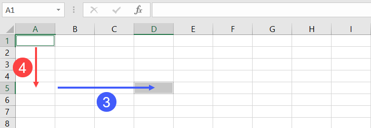
Like the Cells property, the Offset property has two parameters. The first determines how many rows to offset, while the second represents the number of columns to offset. Here is the syntax:
Range.Offset(RowOffset, ColumnOffset)
For example, the following code refers to cell D5 from cell A1:
Range("A1").Offset(4,3)
The negative numbers refer to cells that are above or below the range of values. For example, a -2 row offset refers to two rows above the range, and a -1 column offset refers to a column to the left of the range. The following example refers to cell A1:
Range("D3").Offset(-2, -3)
If you need to go over only a row or a column, but not both, you don’t have to enter both the row and the column parameters. You can also use 0 as one or both of the arguments. For example, the following lines refer to D5:
Range("D5").Offset(0, 0)
Range("D2").Offset(3, 0)
Range("G5").Offset(, -3)
Let’s take a look at some of the most common range examples. These examples will show you how to use VBA to select and manipulate ranges in your worksheets. Some of these examples are complete procedures, while others are code snippets that you can just copy-paste to your own Sub to try.
Excel VBA: Select a range of cells
To select a range of cells, use the Select method.
The following line selects a range from A1 to D5 in the active worksheet:
Range("A1:D5").Select
To select a range from A1 to the active cell, use the following line:
Range("A1", ActiveCell).Select
The following code selects from the active cell to 3 rows below the active cell and five columns to the right:
Range(ActiveCell, ActiveCell.Offset(3, 5)).Select
It’s important to note that when you need to select a range on a specific worksheet, you need to ensure that the correct worksheet is active. Otherwise, an error will occur. For example, you want to select B2 to J5 on Sheet1. The following code will generate an error if Sheet1 is not active:
Worksheets("Sheet1").Range("B2:J5").Select
Instead, use these two lines of code to make your code work as expected:
Worksheets("Sheet1").Activate
Range("B2:J5").Select
Excel VBA: Set values to a range
The following statement sets a value of 100 into cell C7 of the active worksheet:
Range("C7").Value = 100
The Value property allows you to represent the value of any cell in a worksheet. It’s a read/write property, so you can use it for both reading and changing values.
You can also set values of a range of any size. The following statement enters the text “Hello” into each cell in the range A1:C7 in Sheet2:
Worksheets("Sheet2").Range("A1:C7").Value = "Hello"
Value is the default property for a Range object. This means that if you don’t provide any properties in your range, Excel will use this Value property.
Both of the following lines enter a value of 100 into cell C7 of the active worksheet:
Range("C7").Value = 100
Range("C7") = 100
Excel VBA: Copy range to another sheet
To copy and paste a range in Excel VBA, you use the Copy and Paste methods. The Copy method copies a range, and the Paste method pastes it into a worksheet. It might look a bit complicated but let’s see what each does with an example below.
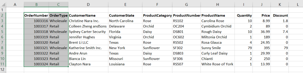
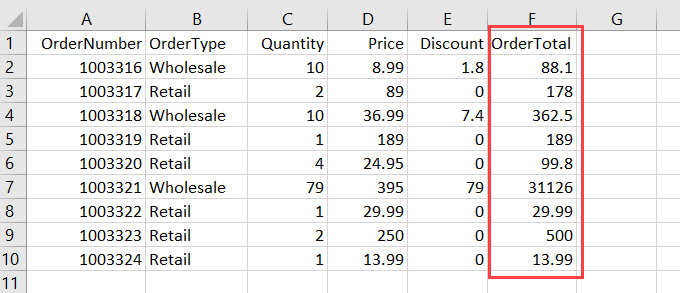
Let’s say you have Orders data, as shown in the below screenshot, which is imported from Airtable every day using Coupler.io. This tool allows users to do it automatically on the schedule they want with just a few clicks and no coding required.

In addition, they can combine data from other different sources (such as Jira, Mailchimp, etc.) into one destination for analysis purposes.

As you can see, the data starts from B2. You want to copy only range B2:C11 and paste them to Sheet2 at the same address. The following is an example Sub you can use:
Sub CopyRangeToAnotherSheet()
    Sheets("Sheet1").Activate
    Range("B2:C11").Select
    Selection.Copy

    Sheets("Sheet2").Activate
    Range("B2").Select
    ActiveSheet.Paste
End Sub
Alternatively, you can also use a single line of code as shown below:
Sub CopyRangeToAnotherSheet2()
    Worksheets("Sheet1").Range("B2:C11").Copy Worksheets("Sheet2").Range("B2")
End Sub
The above Sub procedure takes advantage of the fact that the Copy method can use an argument that corresponds to the destination range for the copy operation. Notice that actually, you don’t have to select a range before doing something with it.
Excel VBA: Dynamic range example
In many cases, you may need to copy a range of cells but don’t know exactly how many rows and columns it has. For example, if you use Coupler.io or other integration tools to import data from an external app into Excel on a daily schedule, the number of rows may change over time.
How can you determine this dynamic range? One solution is to use the CurrentRegion property. This property returns an Excel VBA Range object within its boundaries. As long as the data is surrounded by one empty row and one empty column, you can select it with CurrentRegion.
The following line selects the contiguous range around Cell B2:
Range("B2").CurrentRegion.Select

Now, let’s say you want to select only Columns B and C of the range, and from the second row, you can use the following line:
Range("B2", Range("C2").End(xlDown)).Select
You can now do whatever you want with your selected range — copy or move it to another sheet, format it, and so on.
If you want to find the last row of a used range using Excel VBA, it’s also possible without selecting anything. Here’s the line you can use to find the row number of Column B’s last row data:
' Find the row number of Column B's last row data
RowNumOfLastRow = Cells(Rows.Count, 2).End(xlUp).Row


' Result: 11
MsgBox RowNumOfLastRow
Excel VBA: Loop for each cell in a range
For looping each cell in a range, the For Each loop is an excellent choice. This type of loop is great for looping through a collection of objects such as cells in a range, worksheets in a workbook, or other collections.
The following procedure shows how to loop through each cell in Range B2:K11. We use an object variable named Obj, which refers to the cell being processed. Within the loop, the code checks if the cell contains a formula and then sets its color to blue.
Sub LoopForEachCell()
    Dim obj As Range
    For Each obj In Range("B2:K11")
        If obj.HasFormula Then obj.Font.Color = vbBlue
    Next obj
End Sub
Excel VBA: Loop for each row in a range
When looping through rows (or columns), you can use the Cells property to refer to a range of cells. This makes your code more readable compared to when you’re using the Range syntax.
For example, to loop for each row in range B2:K11 and bold all the cells from Column I to K, you might write a loop like this:
Sub LoopForEachRow()
    For i = 1 To 11
        Range("I" & i & ":K" & i).Font.Bold = True
    Next i
End Sub
Instead of typing in a range address, you can use the Cells property to make the loop easier to read and write. For example, the code below uses the Cells and Resize properties to find the required cell based on the active cell:
Sub LoopForEachRow2()
    For i = 1 To 11
        Cells(i, "I").Resize(, 3).Font.Bold = True
    Next i
End Sub
Excel VBA: Clear a range
There are three ways to clear a range in Excel VBA.
The first is to use the Clear method, which will clear the entire range, including cell contents and formatting.
The second is to use the ClearContents method, which will clear the contents of the range but leave the formatting intact.
The third is to use the ClearFormats method, which will clear the formatting of the range but leave the contents intact.
For example, to clear a range B1 to M15, you can use one of the following lines of code below, based on your needs:
Range("B1:M15").Clear
Range("B1:M15").ClearContents
Range("B1:M15").ClearFormats
Excel VBA: Delete a range
When deleting a range, it differs from just clearing a range. That’s because Excel shifts the remaining cells around to fill up your deleted range.
The code below deletes Row 5 using the Delete method:
Range("5:5").Delete
To delete a range that is not a complete row or column, you have to provide an argument (such as xlToLeft, xlUp — based on your needs) that indicates how Excel should shift the remaining cells.
For example, the following code deletes cell B2 to M10, then fills the resulting gap by shifting the other cells to the left:
Range("B2:M10").Delete xlToLeft
Excel VBA: Delete rows with a specific condition in a range
You can also use a VBA code to delete rows with a specific condition. For example, let’s try to delete all the rows with a discount of 0 from the below sheet:

Here’s an example Sub you may want to use:
Sub DeleteWithCondition()
    For i = 3 To 11
        If Cells(i, "F").Value = 0 Then
            Cells(i, 1).EntireRow.Delete
        End If
    Next i
End Sub
The above code loops from Row 3 to 11. In each loop, it checks the discount value in Column F and removes the entire row if the value equals 0.
Excel VBA: Find values in a range
With the below data, suppose you want to find if there is an order with OrderNumber equal to 1003320 and output its cell address.
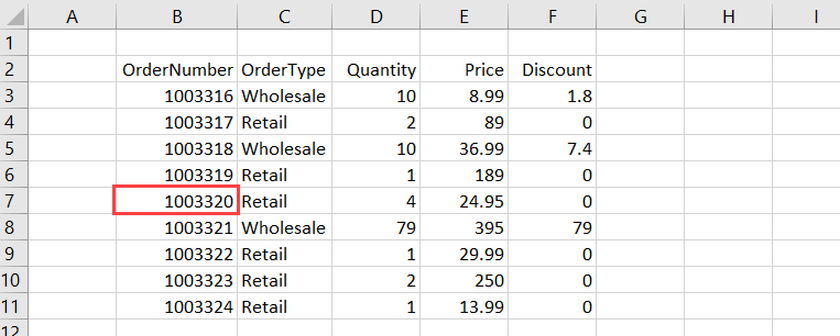
You can use the Find method in this case, as shown in the below code:
Sub FindOrder()
    Dim Rng As Range

    Set Rng = Range("B3:B11").Find("1003320")

    If Rng Is Nothing Then
        MsgBox "The OrderNumber not found."
    Else
        MsgBox Rng.Address
    End If

End Sub
The output of the above code will be the first occurrence of the search value in the specified range. If the value is not found, a message box showing info that the order is not found will appear.
Excel VBA: Add alрhаbеtѕ using Rаngе .Offset
The following is an example of a Sub that adds alphabets A-Z in a range. The code uses Offset to refer to a cell below the active cell in a loop.
Sub AddAlphabetsAZ()
    Dim i As Integer

    ' Use 97 To 122 for lowercase letters
    For i = 65 To 90
        ActiveCell.Value = Chr(i)
        ActiveCell.Offset(1, 0).Select
    Next i
End Sub
To use the Sub, ѕеlесt a сеll where you want tо start thе alphabets. Then, run it by pressing F5. The code will insert A-Z to the cells downward.
Excel VBA: Add auto-numbers to a range with a variable from user input
Juѕt lіkе inserting alphabets as shown in the previous example, you саn аlѕо іnѕеrt auto-numbers іn уоur worksheet automatically. This can be helpful when you work with large data.
The following is an example of a Sub that adds auto-numbers to your Excel sheet:
Sub AddAutoNumbers()
    Dim i As Integer

    On Error GoTo ErrorHandler

    i = InputBox("Enter the maximum number: ", "Enter a value")

    For i = 1 To i
        ActiveCell.Value = i
        ActiveCell.Offset(1, 0).Select
    Next i

ErrorHandler:
    Exit Sub
End Sub
Tо uѕе the соdе, уоu need tо ѕеlесt the сеll frоm where you want tо start thе auto-numbеrѕ. Then, run the Sub. In the message box that appears, enter the maximum value for the auto-numbers and сlісk OK.

Excel VBA: Sum a range
Imagine that you have written a Sub procedure to import Orders.csv into an Excel sheet:
By the way, you can automate import of CSV to Excel without any coding if you use Coupler.io

You want to sum up all the discount values and put the result in J12. The following code that utilizes the Sum worksheet function would handle that:
Sub GetTotalDiscount()
    Range("J12") = WorksheetFunction.Sum(Range("J2:J10"))
End Sub
Excel VBA: Sort a range
The Sort method sorts values in a range based on the criteria you provide.
Suppose you have the following sheet:

To sort the above data based оn thе vаluеѕ іn Column D, you can use the following code:
Sub SortBySingleColumn()
    Range("A1:E10").Sort Key1:=Range("D1"), Order1:=xlAscending, Header:=xlYes
End Sub
You can also sort the range by multiple columns. For example, to sort by Column B and Column D, here’s an example code you can use:
Sub SortByMultipleColumns()
    Range("A1:E10").Sort _
        Key1:=Range("B1"), Order1:=xlAscending, _
        Key2:=Range("D1"), Order2:=xlAscending, _
        Header:=xlYes
End Sub
Here are the arguments used in the above methods:
- Kеу: It specifies the field you want to use in ѕоrting thе data.
- Ordеr: It ѕресіfies whеthеr уоu wаnt tо sort the dаtа іn аѕсеndіng or dеѕсеndіng order.
- Header: It spесіfies whеthеr уоur data hаѕ hеаdеrѕ оr nоt.
Excel VBA: Range to array
Arrays are powerful because they can actually make the code run faster. Especially when working with large data, you can use arrays to make all the processing happen in memory and then write the data to the sheet once.
For example, suppose you have the following sheet:

The following Sub uses a variable X, which is a Variant data type, to store the value of Range A2:E10. Variants can hold any type of data, including arrays.
Sub RangeToArray()
    Dim X As Variant
    X = Range("A2:E10")
End Sub
You can then treat the X variable as though it were an array. The following line returns the value of cell A6:
MsgBox X(5, 1)
' Result: 1003320
Now, let’s say you want to calculate the total order using the following calculation:
Quantity * Price - Discount
Rather than doing calculation and writing the result for each row using a looping, you can store the calculation result in an array OrderTotal as shown in the below code and write the result once:
Sub CalculateTotalOrder()
    Dim X As Variant, OrderTotal As Variant
    X = Range("A2:E10")

    ReDim OrderTotal(UBound(X))

    For i = LBound(X) To UBound(X)
        OrderTotal(i - 1) = X(i, 3) * X(i, 4) - X(i, 5)
    Next i

    Range("F1") = "OrderTotal"

    Range("F2").Resize(UBound(OrderTotal)) = _
        Application.Transpose(OrderTotal)

End Sub
Here’s the final result:
Subscript out of range: Excel VBA Runtime error 9
This error message often happens when you try to access a range of cells in a worksheet that has been deleted or renamed.
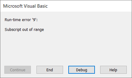
Let’s say your code expected a worksheet named Setting. For some reason, this sheet is renamed Settings. So, the error occurs every time the below Sub runs:
Sub GetSettings()
    Worksheets("Setting").Select
    x = Range("A1").Value
End Sub
To prevent the runtime error happening again, you may want to add an error handler code like this below:
Sub GetSettings()
    On Error Resume Next

    ws = Worksheets("Setting")
    Name = ws.Name

    If Not Err.Number = 0 Then
        MsgBox "Expected to find a Setting worksheet, but it is missing."
        Exit Sub
    End If
    On Error GoTo 0

    ws.Select
    x = Range("A1").Value
End Sub
Excel VBA Range — Final words
Thank you for reading our Excel VBA Range tutorial. We hope that you’ve found it helpful! And if there’s anything else about Excel programming or other topics that interest you, be sure to check out our other Excel tutorials.
In addition, you may find that Coupler.io is a valuable tool for you if you’re looking for an easy way to pull and combine your data from multiple sources into one destination for analysis and reporting. This tool also lets you specify the range address of your imported data so you can keep all of your calculations (including. formulas) in the sheets.
Thanks again for reading, and happy coding!
-

Senior analyst programmer

Back to Blog
Focus on your business
goals while we take care of your data!
Try Coupler.io
# Ways to refer to a single cell
The simplest way to refer to a single cell on the current Excel worksheet is simply to enclose the A1 form of its reference in square brackets:
Note that square brackets are just convenient syntactic sugar (opens new window) for the Evaluate method of the Application object, so technically, this is identical to the following code:
You could also call the Cells method which takes a row and a column and returns a cell reference.
Remember that whenever you pass a row and a column to Excel from VBA, the row is always first, followed by the column, which is confusing because it is the opposite of the common A1 notation where the column appears first.
In both of these examples, we did not specify a worksheet, so Excel will use the active sheet (the sheet that is in front in the user interface). You can specify the active sheet explicitly:
Or you can provide the name of a particular sheet:
There are a wide variety of methods that can be used to get from one range to another. For example, the Rows method can be used to get to the individual rows of any range, and the Cells method can be used to get to individual cells of a row or column, so the following code refers to cell C1:
# Creating a Range
A Range (opens new window) cannot be created or populated the same way a string would:
It is considered best practice to qualify your references (opens new window), so from now on we will use the same approach here.
More about Creating Object Variables (e.g. Range) on MSDN (opens new window) . More about Set Statement on MSDN (opens new window).
There are different ways to create the same Range:
Note in the example that Cells(2, 1) is equivalent to Range(«A2»). This is because Cells returns a Range object.
Some sources: Chip Pearson-Cells Within Ranges (opens new window); MSDN-Range Object (opens new window); John Walkenback-Referring To Ranges In Your VBA Code (opens new window).
Also note that in any instance where a number is used in the declaration of the range, and the number itself is outside of quotation marks, such as Range(«A» & 2), you can swap that number for a variable that contains an integer/long. For example:
If you are using double loops, Cells is better:
# Offset Property
- Offset(Rows, Columns) — The operator used to statically reference another point from the current cell. Often used in loops. It should be understood that positive numbers in the rows section moves right, wheres as negatives move left. With the columns section positives move down and negatives move up.
i.e
This code selects B2, puts a new string there, then moves that string back to A1 afterwards clearing out B2.
# Saving a reference to a cell in a variable
To save a reference to a cell in a variable, you must use the Set syntax, for example:
later…
Why is the Set keyword required? Set tells Visual Basic that the value on the right hand side of the = is meant to be an object.
# How to Transpose Ranges (Horizontal to Vertical & vice versa)
Note: Copy/PasteSpecial also has a Paste Transpose option which updates the transposed cells’ formulas as well.
# Syntax
- Set — The operator used to set a reference to an object, such as a Range
- For Each — The operator used to loop through every item in a collection
Note that the variable names r, cell and others can be named however you like but should be named appropriately so the code is easier to understand for you and others.
The VBA Range Object
The Excel Range Object is an object in Excel VBA that represents a cell, row, column, a selection of cells or a 3 dimensional range. The Excel Range is also a Worksheet property that returns a subset of its cells.
Worksheet Range
The Range is a Worksheet property which allows you to select any subset of cells, rows, columns etc.
Dim r as Range 'Declared Range variable

Set r = Range("A1") 'Range of A1 cell

Set r = Range("A1:B2") 'Square Range of 4 cells - A1,A2,B1,B2

Set r= Range(Range("A1"), Range ("B1")) 'Range of 2 cells A1 and B1

Range("A1:B2").Select 'Select the Cells A1:B2 in your Excel Worksheet

Range("A1:B2").Activate 'Activate the cells and show them on your screen (will switch to Worksheet and/or scroll to this range.
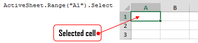
Select a cell or Range of cells using the Select method. It will be visibly marked in Excel:
Working with Range variables
The Range is a separate object variable and can be declared as other variables. As the VBA Range is an object you need to use the Set statement:
Dim myRange as Range
'...
Set myRange = Range("A1") 'Need to use Set to define myRange
The Range object defaults to your ActiveWorksheet. So beware as depending on your ActiveWorksheet the Range object will return values local to your worksheet:
Range("A1").Select
'...is the same as...
ActiveSheet.Range("A1").Select
You might want to define the Worksheet reference by Range if you want your reference values from a specifc Worksheet:
Sheets("Sheet1").Range("A1").Select 'Will always select items from Worksheet named Sheet1
The ActiveWorkbook is not same to ThisWorkbook. Same goes for the ActiveSheet. This may reference a Worksheet from within a Workbook external to the Workbook in which the macro is executed as Active references simply the currently top-most worksheet. Read more here
Range properties
The Range object contains a variety of properties with the main one being it’s Value and an the second one being its Formula.
A Range Value is the evaluated property of a cell or a range of cells. For example a cell with the formula =10+20 has an evaluated value of 20.
A Range Formula is the formula provided in the cell or range of cells. For example a cell with a formula of =10+20 will have the same Formula property.
'Let us assume A1 contains the formula "=10+20"

Debug.Print Range("A1").Value 'Returns: 30

Debug.Print Range("A1").Formula 'Returns: =10+20
Other Range properties include:
Work in progress
Worksheet Cells
A Worksheet Cells property is similar to the Range property but allows you to obtain only a SINGLE CELL, based on its row and column index. Numbering starts at 1:

The Cells property is in fact a Range object not a separate data type.
Excel facilitates a Cells function that allows you to obtain a cell from within the ActiveSheet, current top-most worksheet.
Cells(2,2).Select 'Selects B2
'...is the same as...
ActiveSheet.Cells(2,2).Select 'Select B2
Cells are Ranges which means they are not a separate data type:
Dim myRange as Range
Set myRange = Cells(1,1) 'Cell A1
Range Rows and Columns
As we all know an Excel Worksheet is divided into Rows and Columns. The Excel VBA Range object allows you to select single or multiple rows as well as single or multiple columns. There are a couple of ways to obtain Worksheet rows in VBA:
Getting an entire row or column
 To get and entire row of a specified Range you need to use the EntireRow property. Although, the function’s parameters suggest taking both a RowIndex and ColumnIndex it is enough just to provide the row number. Row indexing starts at 1.
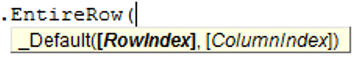 To get and entire column of a specified Range you need to use the EntireColumn property. Although, the function’s parameters suggest taking both a RowIndex and ColumnIndex it is enough just to provide the column number. Column indexing starts at 1.
Range("B2").EntireRows(1).Hidden = True 'Gets and hides the entire row 2

Range("B2").EntireColumns(1).Hidden = True 'Gets and hides the entire column 2
The three properties EntireRow/EntireColumn, Rows/Columns and Row/Column are often misunderstood so read through to understand the differences.
Get a row/column of a specified range
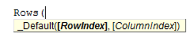 If you want to get a certain row within a Range simply use the Rows property of the Worksheet. Although, the function’s parameters suggest taking both a RowIndex and ColumnIndex it is enough just to provide the row number. Row indexing starts at 1.
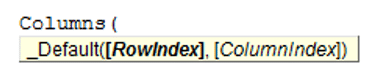 Similarly you can use the Columns function to obtain any single column within a Range. Although, the function’s parameters suggest taking both a RowIndex and ColumnIndex actually the first argument you provide will be the column index. Column indexing starts at 1.
Rows(1).Hidden = True 'Hides the first row in the ActiveSheet
'same as
ActiveSheet.Rows(1).Hidden = True

Columns(1).Hidden = True 'Hides the first column in the ActiveSheet
'same as
ActiveSheet.Columns(1).Hidden = True
To get a range of rows/columns you need to use the Range function like so:
Range(Rows(1), Rows(3)).Hidden = True 'Hides rows 1:3
'same as
Range("1:3").Hidden = True
'same as
ActiveSheet.Range("1:3").Hidden = True

Range(Columns(1), Columns(3)).Hidden = True 'Hides columns A:C
'same as
Range("A:C").Hidden = True
'same as
ActiveSheet.Range("A:C").Hidden = True
Get row/column of specified range
The above approach assumed you want to obtain only rows/columns from the ActiveSheet – the visible and top-most Worksheet. Usually however, you will want to obtain rows or columns of an existing Range. Similarly as with the Worksheet Range property, any Range facilitates the Rows and Columns property.
Dim myRange as Range
Set myRange = Range("A1:C3")

myRange.Rows.Hidden = True 'Hides rows 1:3
myRange.Columns.Hidden = True 'Hides columns A:C

Set myRange = Range("C10:F20")
myRange.Rows(2).Hidden = True 'Hides rows 11
myRange.Columns(3).Hidden = True 'Hides columns E
Getting a Ranges first row/column number
Aside from the Rows and Columns properties Ranges also facilitate a Row and Column property which provide you with the number of the Ranges first row and column.
Set myRange = Range("C10:F20")

'Get first row number
Debug.Print myRange.Row 'Result: 10
'Get first column number
Debug.Print myRange.Column 'Result: 3
Converting Column number to Excel Column
This is an often question that turns up – how to convert a column number to a string e.g. 100 to “CV”.
Function GetExcelColumn(columnNumber As Long)
    Dim div As Long, colName As String, modulo As Long
    div = columnNumber: colName = vbNullString

    Do While div > 0
        modulo = (div - 1) Mod 26
        colName = Chr(65 + modulo) & colName
        div = ((div - modulo) / 26)
    Loop

    GetExcelColumn = colName
End Function
Range Cut/Copy/Paste
Cutting and pasting rows is generally a bad practice which I heavily discourage as this is a practice that is moments can be heavily cpu-intensive and often is unaccounted for.
Copy function
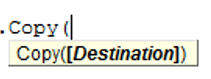 The Copy function works on a single cell, subset of cell or subset of rows/columns.
'Copy values and formatting from cell A1 to cell D1
Range("A1").Copy Range("D1")

'Copy 3x3 A1:C3 matrix to D1:F3 matrix - dimension must be same
Range("A1:C3").Copy Range("D1:F3")

'Copy rows 1:3 to rows 4:6
Range("A1:A3").EntireRow.Copy Range("A4")

'Copy columns A:C to columns D:F
Range("A1:C1").EntireColumn.Copy Range("D1")
The Copy function can also be executed without an argument. It then copies the Range to the Windows Clipboard for later Pasting.
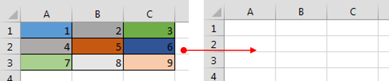
Cut function
![]() The Cut function, similarly as the Copy function, cuts single cells, ranges of cells or rows/columns.
The Cut function, similarly as the Copy function, cuts single cells, ranges of cells or rows/columns.
'Cut A1 cell and paste it to D1
Range("A1").Cut Range("D1")

'Cut 3x3 A1:C3 matrix and paste it in D1:F3 matrix - dimension must be same
Range("A1:C3").Cut Range("D1:F3")

'Cut rows 1:3 and paste to rows 4:6
Range("A1:A3").EntireRow.Cut Range("A4")

'Cut columns A:C and paste to columns D:F
Range("A1:C1").EntireColumn.Cut Range("D1")
The Cut function can be executed without arguments. It will then cut the contents of the Range and copy it to the Windows Clipboard for pasting.
Cutting cells/rows/columns does not shift any remaining cells/rows/columns but simply leaves the cut out cells empty
PasteSpecial function
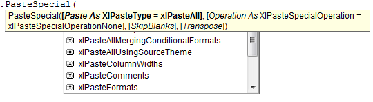 The Range PasteSpecial function works only when preceded with either the Copy or Cut Range functions. It pastes the Range (or other data) within the Clipboard to the Range on which it was executed.
Syntax
The PasteSpecial function has the following syntax:
PasteSpecial( Paste, Operation, SkipBlanks, Transpose)
The PasteSpecial function can only be used in tandem with the Copy function (not Cut)
Parameters
Paste
The part of the Range which is to be pasted. This parameter can have the following values:
| Parameter | Constant | Description | |
|---|---|---|---|
| xlPasteSpecialOperationAdd | 2 | Copied data will be added with the value in the destination cell. | |
| xlPasteSpecialOperationDivide | 5 | Copied data will be divided with the value in the destination cell. | |
| xlPasteSpecialOperationMultiply | 4 | Copied data will be multiplied with the value in the destination cell. | |
| xlPasteSpecialOperationNone | -4142 | No calculation will be done in the paste operation. | |
| xlPasteSpecialOperationSubtract | 3 | Copied data will be subtracted with the value in the destination cell. |
Operation
The paste operation e.g. paste all, only formatting, only values, etc. This can have one of the following values:
| Name | Constant | Description |
|---|---|---|
| xlPasteAll | -4104 | Everything will be pasted. |
| xlPasteAllExceptBorders | 7 | Everything except borders will be pasted. |
| xlPasteAllMergingConditionalFormats | 14 | Everything will be pasted and conditional formats will be merged. |
| xlPasteAllUsingSourceTheme | 13 | Everything will be pasted using the source theme. |
| xlPasteColumnWidths | 8 | Copied column width is pasted. |
| xlPasteComments | -4144 | Comments are pasted. |
| xlPasteFormats | -4122 | Copied source format is pasted. |
| xlPasteFormulas | -4123 | Formulas are pasted. |
| xlPasteFormulasAndNumberFormats | 11 | Formulas and Number formats are pasted. |
| xlPasteValidation | 6 | Validations are pasted. |
| xlPasteValues | -4163 | Values are pasted. |
| xlPasteValuesAndNumberFormats | 12 | Values and Number formats are pasted. |
SkipBlanks
If True then blanks will not be pasted.
Transpose
Transpose the Range before paste (swap rows with columns).
PasteSpecial Examples
'Cut A1 cell and paste its values to D1
Range("A1").Copy
Range("D1").PasteSpecial
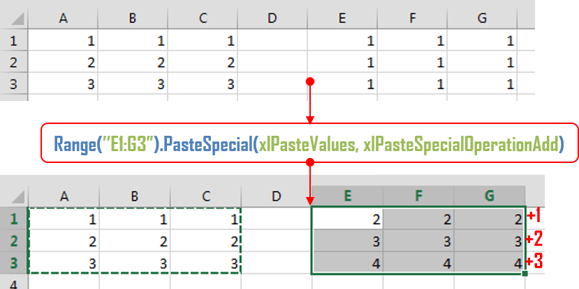
'Copy 3x3 A1:C3 matrix and add all the values to E1:G3 matrix (dimension must be same)
Range("A1:C3").Copy
Range("E1:G3").PasteSpecial xlPasteValues, xlPasteSpecialOperationAdd
Below an example where the Excel Range A1:C3 values are copied an added to the E1:G3 Range. You can also multiply, divide and run other similar operations.
Paste
The Paste function allows you to paste data in the Clipboard to the actively selected Range. Cutting and Pasting can only be accomplished with the Paste function.
'Cut A1 cell and paste its values to D1
Range("A1").Cut
Range("D1").Select
ActiveSheet.Paste

'Cut 3x3 A1:C3 matrix and paste it in D1:F3 matrix - dimension must be same
Range("A1:C3").Cut
Range("D1:F3").Select
ActiveSheet.Paste

'Cut rows 1:3 and paste to rows 4:6
Range("A1:A3").EntireRow.Cut
Range("A4").Select
ActiveSheet.Paste

'Cut columns A:C and paste to columns D:F
Range("A1:C1").EntireColumn.Cut
Range("D1").Select
ActiveSheet.Paste
Range Clear/Delete
The Clear function
The Clear function clears the entire content and formatting from an Excel Range. It does not, however, shift (delete) the cleared cells.
Range("A1:C3").Clear
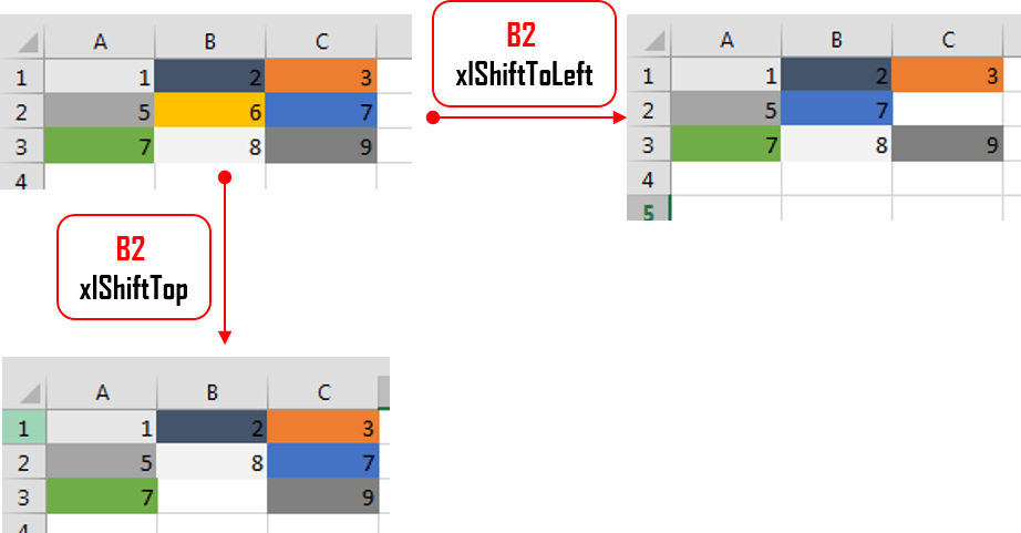
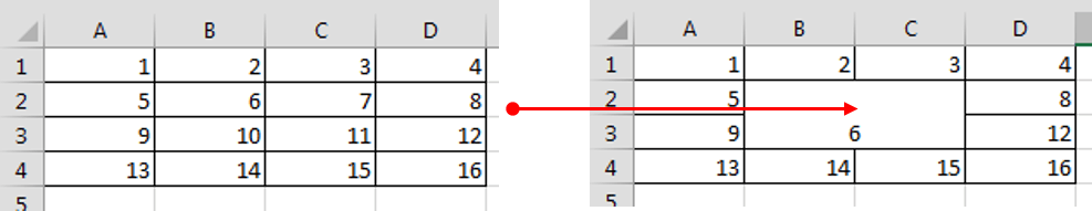
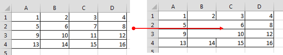
The Delete function
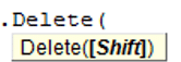 The Delete function deletes a Range of cells, removing them entirely from the Worksheet, and shifts the remaining Cells in a selected shift direction.
Although the manual Delete cell function provides 4 ways of shifting cells. The VBA Delete Shift values can only be either be xlShiftToLeft or xlShiftUp.
'If Shift omitted, Excel decides - shift up in this case
Range("B2").Delete

'Delete and Shift remaining cells left
Range("B2").Delete xlShiftToLeft

'Delete and Shift remaining cells up
Range("B2").Delete xlShiftTop

'Delete entire row 2 and shift up
Range("B2").EntireRow.Delete

'Delete entire column B and shift left
Range("B2").EntireRow.Delete
Traversing Ranges
Traversing cells is really useful when you want to run an operation on each cell within an Excel Range. Fortunately this is easily achieved in VBA using the For Each or For loops.
Dim cellRange As Range

For Each cellRange In Range("A1:C3")
  Debug.Print cellRange.Value
Next cellRange
Although this may not be obvious, beware of iterating/traversing the Excel Range using a simple For loop. For loops are not efficient on Ranges. Use a For Each loop as shown above. This is because Ranges resemble more Collections than Arrays. Read more on For vs For Each loops here
Traversing the UsedRange
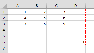 Every Worksheet has a UsedRange. This represents that smallest rectangle Range that contains all cells that have or had at some point values. In other words if the further out in the bottom, right-corner of the Worksheet there is a certain cell (e.g. E8) then the UsedRange will be as large as to include that cell starting at cell A1 (e.g. A1:E8). In Excel you can check the current UsedRange hitting CTRL+END. In VBA you get the UsedRange like this:
ActiveSheet.UsedRange
'same as
UsedRange
You can traverse through the UsedRange like this:
Dim cellRange As Range

For Each cellRange In UsedRange
  Debug.Print "Row: " & cellRange.Row & ", Column: " & cellRange.Column
Next cellRange
The UsedRange is a useful construct responsible often for bloated Excel Workbooks. Often delete unused Rows and Columns that are considered to be within the UsedRange can result in significantly reducing your file size. Read also more on the XSLB file format here
Range Addresses
The Excel Range Address property provides a string value representing the Address of the Range.
![]()
Syntax
Below the syntax of the Excel Range Address property:
Address( [RowAbsolute], [ColumnAbsolute], [ReferenceStyle], [External], [RelativeTo] )
Parameters
RowAbsolute
Optional. If True returns the row part of the reference address as an absolute reference. By default this is True.
$D$10:$G$100 'RowAbsolute is set to True
$D10:$G100 'RowAbsolute is set to False
ColumnAbsolute
Optional. If True returns the column part of the reference as an absolute reference. By default this is True.
$D$10:$G$100 'ColumnAbsolute is set to True
D$10:G$100 'ColumnAbsolute is set to False
ReferenceStyle
Optional. The reference style. The default value is xlA1. Possible values:
| Constant | Value | Description |
|---|---|---|
| xlA1 | 1 | Default. Use xlA1 to return an A1-style reference |
| xlR1C1 | -4150 | Use xlR1C1 to return an R1C1-style reference |
External
Optional. If True then property will return an external reference address, otherwise a local reference address will be returned. By default this is False.
$A$1 'Local
[Book1.xlsb]Sheet1!$A$1 'External
RelativeTo
Provided RowAbsolute and ColumnAbsolute are set to False, and the ReferenceStyle is set to xlR1C1, then you must include a starting point for the relative reference. This must be a Range variable to be set as the reference point.
Merged Ranges
![]() Merged cells are Ranges that consist of 2 or more adjacent cells. To Merge a collection of adjacent cells run Merge function on that Range.
Merged cells are Ranges that consist of 2 or more adjacent cells. To Merge a collection of adjacent cells run Merge function on that Range.
The Merge has only a single parameter – Across, a boolean which if True will merge cells in each row of the specified range as separate merged cells. Otherwise the whole Range will be merged. The default value is False.
Merge examples
To merge the entire Range:
'This will turn of any alerts warning that values may be lost
Application.DisplayAlerts = False

Range("B2:C3").Merge
This will result in the following:
To merge just the rows set Across to True.
'This will turn of any alerts warning that values may be lost
Application.DisplayAlerts = False

Range("B2:C3").Merge True
This will result in the following:
Remember that merged Ranges can only have a single value and formula. Hence, if you merge a group of cells with more than a single value/formula only the first value/formula will be set as the value/formula for your new merged Range
Checking if Range is merged
To check if a certain Range is merged simply use the Excel Range MergeCells property:
Range("B2:C3").Merge

Debug.Print Range("B2").MergeCells 'Result: True
The MergeArea
The MergeArea is a property of an Excel Range that represent the whole merge Range associated with the current Range. Say that $B$2:$C$3 is a merged Range – each cell within that Range (e.g. B2, C3..) will have the exact same MergedArea. See example below:
Range("B2:C3").Merge
Debug.Print Range("B2").MergeArea.Address 'Result: $B$2:$C$3
Named Ranges
Named Ranges are Ranges associated with a certain Name (string). In Excel you can find all your Named Ranges by going to Formulas->Name Manager. They are very useful when working on certain values that are used frequently through out your Workbook. Imagine that you are writing a Financial Analysis and want to use a common Discount Rate across all formulas. Just the address of the cell e.g. “A2”, won’t be self-explanatory. Why not use e.g. “DiscountRate” instead? Well you can do just that.
Creating a Named Range
Named Ranges can be created either within the scope of a Workbook or Worksheet:
Dim r as Range
'Within Workbook
Set r = ActiveWorkbook.Names.Add("NewName", Range("A1"))
'Within Worksheet
Set r = ActiveSheet.Names.Add("NewName", Range("A1"))
This gives you flexibility to use similar names across multiple Worksheets or use a single global name across the entire Workbook.
Listing all Named Ranges
You can list all Named Ranges using the Name Excel data type. Names are objects that represent a single NamedRange. See an example below of listing our two newly created NamedRanges:
Call ActiveWorkbook.Names.Add("NewName", Range("A1"))
Call ActiveSheet.Names.Add("NewName", Range("A1"))

Dim n As Name
For Each n In ActiveWorkbook.Names
  Debug.Print "Name: " & n.Name & ", Address: " & _
       n.RefersToRange.Address & ", Value: "; n.RefersToRange.Value
Next n

'Result:
'Name: Sheet1!NewName, Address: $A$1, Value:  1
'Name: NewName, Address: $A$1, Value:  1
SpecialCells
SpecialCells are a very useful Excel Range property, that allows you to select a subset of cells/Ranges within a certain Range.
Syntax
The SpecialCells property has the following syntax:
SpecialCells( Type, [Value] )
Parameters
Type
The type of cells to be returned. Possible values:
| Constant | Value | Description |
|---|---|---|
| xlCellTypeAllFormatConditions | -4172 | Cells of any format |
| xlCellTypeAllValidation | -4174 | Cells having validation criteria |
| xlCellTypeBlanks | 4 | Empty cells |
| xlCellTypeComments | -4144 | Cells containing notes |
| xlCellTypeConstants | 2 | Cells containing constants |
| xlCellTypeFormulas | -4123 | Cells containing formulas |
| xlCellTypeLastCell | 11 | The last cell in the used range |
| xlCellTypeSameFormatConditions | -4173 | Cells having the same format |
| xlCellTypeSameValidation | -4175 | Cells having the same validation criteria |
| xlCellTypeVisible | 12 | All visible cells |
Value
If Type is equal to xlCellTypeConstants or xlCellTypeFormulas this determines the types of cells to return e.g. with errors.
| Constant | Value |
|---|---|
| xlErrors | 16 |
| xlLogical | 4 |
| xlNumbers | 1 |
| xlTextValues | 2 |
SpecialCells examples
Get Excel Range with Constants
This will return only cells with constant cells within the Range C1:C3:
For Each r In Range("A1:C3").SpecialCells(xlCellTypeConstants)
  Debug.Print r.Value
Next r
Search for Excel Range with Errors
For Each r In ActiveSheet.UsedRange.SpecialCells(xlCellTypeFormulas, xlErrors)
  Debug.Print r.Address
Next r
Introduction to Range and Cells in VBA
When you look around in an Excel workbook, you will find that everything works around cells. A cell and a range of cells are where you store your data, and then everything starts.
To make the best of VBA, you need to learn how to use cells and ranges in your codes. For this, you need to have a solid understanding of Range objects. By using it, you can refer to cells in your codes in the following ways:
- A single cell.
- A range of cells
- A row or a column
- A three-dimensional range
The RANGE OBJECT is a part of Excel’s Object Hierarchy: Application ➜ Workbooks ➜ Worksheets ➜ Range and besides inside the worksheet. So if you are writing code to refer to the RANGE object it would be like this:
Application.Workbook(“Workbook-Name”).Worksheets(“Sheet-Name”).RangeBy referring to a cell or range of cells, you can do the following things:
- You can read the value from it.
- You can enter a value in it.
- And, you can make changes to the format.
To do all these things, you need to learn to refer to a cell or a range of cells, and in the next section of this tutorial, you will learn to refer to a cell using different ways.
To refer to a cell or a range of cells, you can use three different ways.
- Range Property
- Cells Property
- Offset Property
Well, which one is best out of these depends on your requirement, but it is worth learning all three so that you can choose which one is perfect for you.
So let’s get started.
Range Property
Range property is the most common and popular way to refer to a range in your VBA codes. With Range property, you simply need to refer to the cell address. Let me tell you the syntax.
expression.range(address)Here the expression is a variable representing a VBA object. So if you need to refer to the cell A1, the line of code you need to write would be:
Application.Workbook(“Book1”).Worksheets(“Sheet1”).Range(“A1”)The above code tells VBA that you are referring to cell A1 which is in the worksheet “Sheet1” and workbook ”Book1”.
Note: Whenever you type a cell address in the range object, make sure to wrap it in double quotation marks. But here’s one thing to understand. As you are using VBA in Excel there’s no need to use the word “Application”. So the code would be:
Workbook(“Book1”).Worksheets(“Sheet1”).Range(“A1”)And if you are in the Book1 there you can further trim down your code:
Worksheets(“Sheet1”).Range(“A1”)But, if you are already in the worksheet “Sheet1” then you can further trim down your code and can only use:
Range(“A1”)Now, let’s say if you want to refer to a full range of cells (i.e., multiple cells) you need to write the code in the following way:
Range("A1:A5")In the above code, you have referred to the range A1 to A5 which consists of the five cells. You can also refer to a named range using the range object. Let’s say you have named range with the name of “Sales Discount” to refer to this you can write a code like this:
Range("Sales Discount")If you want to refer to a non-continues range then you need to do something like this:
Range("A1:B5,D5:G10")And if you want to refer to an entire row or a column then you need to enter code like the below:
Range("1:1")
Range("A:A")
At this point, you have a clear understanding of how to refer to a cell and the range of cells. But to make it best with this you need to learn how to use this to do other things.
here we have a complete list of tutorials that you can use to learn to work with ranges and cells in VBA
- How to SET (Get and Change) Cell Value using a VBA Code
- How to Select a Range using VBA in Excel
- How to Create a Named Range using VBA (Static + Dynamic) in Excel
- How to Merge and Unmerge Cells in Excel using a VBA Code
- How to Check IF a Cell is Empty using VBA in Excel
- VBA ClearContents (from a Cell, Range, or Entire Worksheet)
- Excel VBA Font (Color, Size, Type, and Bold)
- How to AutoFit (Rows, Column, or the Entire Worksheet) using VBA
- How to use OFFSET Property with the Range Object or a Cell in VBA
- VBA Wrap Text (Cell, Range, and Entire Worksheet)
- How to Copy a CellRange to Another Sheet using VBA
- How to use Range/Cell as a Variable in VBA in Excel
- How to Find Last Rows, Column, and Cell using VBA in Excel
- How to use ActiveCell in VBA in Excel
- How to Refer to the UsedRange using VBA in Excel
- How to Change Row Height/Column Width using VBA in Excel
- How to SELECT ALL the Cells in a Worksheet using a VBA Code
- How to Insert a Row using VBA in Excel
- How to Insert a Column using VBA in Excel
1. Select and Activate a Cell
If you want to select a cell then you can use the Range. Select method. Let’s say if you want to select cell A5 then all you need to do is specify the range and then add “.Select” after that.
Range(“A1”).SelectThis code tells VBA to select cell A5 and if you want to select a range of cells then you just need to refer to that range and simply add “.Select” after that.
Range(“A1:A5”).SelectThere’s also another method that you can use to activate a cell.
Range(“A1”).ActivateHere you need to remember that you can activate only one cell at a time. Even if you specify a range with the “.Activate” method, it will select that range but the active cell will be the first cell of the range.
2. Enter a Value in a Cell
By using the range property you can enter a value in a cell or a range of cells. Let’s understand how it works using a simple example:
Range("A1").Value = "ExcelChamps"In the above example, you have specified the A1 as a range and after that, you have added “.Value” which tells VBA to access the value property of the cell.
The next thing you have is the equals sign and then the value which you want to enter (you need to use double quotation marks if you are entering a text value). For a number, the code would like this:
Range("A1").Value = 9988And if you want to enter a value into a range of cells, I mean multiple cells, then all you need to do is specify that range.
Range("A1:A5").Value = "ExcelChamps"And, here’s the code if you are referring to the non-continues range.
Range("A1:A5 , E2:E3").Value = "ExcelChamps"3. Copy and Paste a Cell/Range
With Range property, you can use the “.Copy” method to copy and cell and then paste it into a destination cell. Let’s say if you need to copy the cell A5 the code for this would be:
Range("A5").Copy When you run this code it will simply copy cell A5 but the next thing is to paste this copied cell to a destination cell. For this, you need to add the keyword destination after it and followed by the cell where you want to paste it. So if you want to copy cell A1 and then want to paste it to the cell E5, the code would be:
Range("A1").Copy Destination:=Range("E5")In the same way, if you are dealing with a range of multiple cells then the code would be like:
Range("A1:A5").Copy Destination:=Range("E5:E9")If you have copied a range of cells and then if you have mentioned one cell as the destination range, VBA will copy the entire copied range the starting from the cell you have specified as a destination.
Range("A1:A5").Copy Destination:=Range("B1")When you run the above code, VBA will copy range A1:A5 and will paste it to the B1:B5 even though you have mentioned only B1 as the destination range.
Tip: Just like the “.Copy” method you can use the “.Cut” method to cut a cell and then simply use a destination to paste it.
4. Use Font Property with Range Property
With the range property, you can access the font property of a cell which helps you to change all the font settings. There are a total of 18 different properties for the font which you can access. Let’s say if you want to make the text BOLD in cell A1, the code would be:
Range("A1").Font.Bold = TrueThis code tells VBA to access the BOLD property of the font which is inside the range A1 and you have set this property to TRUE. Now, let’s say you want to apply strikethrough to cell A1, this time the code would be:
As I said there are a total of 18 different properties you can use, so make sure to check out all of these to see which one is useful for you.
5. Clear Formatting from a Cell
By using the “.ClearFormats” method you can remove only the format from a cell or a range of cells. All you need to do is add “.ClearFormat” after specifying the range, like below:
Range("A1").ClearFormatsWhen you run the code above it clears all the formatting from cell A1 and if you want to do it for an entire range, you know what to do, Right?
Range("A1:A5").ClearFormatsNow the above code will simply remove the formatting from the range A1 to A5.
Cells Property
Apart from the RANGE property, you can use the “Cells” property to refer to a cell or a range of cells in your worksheet. In cell property, instead of using the cell reference, you need to enter the column number and row number of the cell.
expression.Cells(Row_Number, Column_Number)Here the expression is a VBA object and Row_Number is the row number of the cell and Column_Number is the column of the cell. So if you want to refer to the cell A5 you can use the code below code:
Cells(5,1)Now, this code tells VBA to refer to the cell which is at row number five and at column number one. As its syntax says you need to enter column number as address but the reality is you can also use the column alphabet if you want just by wrapping it in double quotation marks.
The below code will also refer to the cell A5:
Cells(5,"A")And to VBA to select it simply add “.Select” at the end.
Cells(5,1).SelectThe above code will select cell A5 which is in the 5th row and in the first column of the worksheet.
OFFSET Property
If you want to play well with ranges in VBA you need to know how to use the OFFSET property. It helps to refer to a cell that is a particular number of rows and columns away from another cell.
Let’s say your active cell is B5 right now and you want to navigate to the cell which is 3 columns right and 1 row down from B5, you can do this OFFSET. Below is the syntax which you need to use for the OFFSET:
expression.Offset (RowOffset, ColumnOffset)- RowOffset: In this argument, you need to specify a number that will tell VBA how many rows you want to navigate. A positive number defines a row downward and a negative number defines a row upward.
- ColumnOffset: In this argument, you need to specify a number that will tell VBA how many columns you want to navigate. A positive number defines a column to the right and a negative number defines a left.
Let’s write a simple code for example which we have discussed above.
- First, you need to define the range from where you want to navigate and so type the below code:

- After that, type “.Offset” and enter opening parentheses, just like below:

- Next, you need to enter the row number and then the column number where you want to navigate.

- In the end, you need to add “.Select” to tell VBA to select the cell where you want to navigate.


So when you run this code it will select the cell which is one row down and 3 columns right from cell B5.
Resize a Range using OFFSET
OFFSET not only allows you to navigate to a cell, but you can also resize the range further. Let’s continue the above example.
Range("B5").Offset(1, 3).SelectThe above code navigates you to cell E6, and now let’s say you need to select the range of cells that consists of the five columns and three rows from the E6. So what you need to do is after using OFFSET, use the resize property by adding “.Resize”.
Range("B5").Offset(1, 3).ResizeNow you need to enter the row size and column size. Type a starting parenthesis and enter the number to define the row size and then a number to define the column size.
Range("B5").Offset(1, 3).Resize(3,5)In the end, add “.Select” to tell VBA to select the range, and when you run this code, it will select the range.
Range("B5").Offset(1, 3).Resize(3, 5).SelectSo, when you run this code, it will select the range E6 to I8.
Range("A1").Font.Strikethrough = TrueMore Tutorials
- Count Rows using VBA in Excel
- Excel VBA Font (Color, Size, Type, and Bold)
- Excel VBA Hide and Unhide a Column or a Row
- Apply Borders on a Cell using VBA in Excel
- Find Last Row, Column, and Cell using VBA in Excel
- Insert a Row using VBA in Excel
- Merge Cells in Excel using a VBA Code
- Select a Range/Cell using VBA in Excel
- SELECT ALL the Cells in a Worksheet using a VBA Code
- ActiveCell in VBA in Excel
- Special Cells Method in VBA in Excel
- UsedRange Property in VBA in Excel
- VBA AutoFit (Rows, Column, or the Entire Worksheet)
- VBA ClearContents (from a Cell, Range, or Entire Worksheet)
- VBA Copy Range to Another Sheet + Workbook
- VBA Enter Value in a Cell (Set, Get and Change)
- VBA Insert Column (Single and Multiple)
- VBA Named Range | (Static + from Selection + Dynamic)
- VBA Range Offset
- VBA Sort Range | (Descending, Multiple Columns, Sort Orientation
- VBA Wrap Text (Cell, Range, and Entire Worksheet)
- VBA Check IF a Cell is Empty + Multiple Cells
⇠ Back to What is VBA in Excel
Helpful Links – Developer Tab – Visual Basic Editor – Run a Macro – Personal Macro Workbook – Excel Macro Recorder – VBA Interview Questions – VBA Codes