
17 авг. 2022 г.
читать 2 мин
U-критерий Манна-Уитни (иногда называемый критерием суммы рангов Уилкоксона) используется для сравнения различий между двумя выборками, когда распределение выборки не является нормальным, а размеры выборки малы (n < 30).
Он считается непараметрическим эквивалентом двухвыборочного t-критерия .
В этом руководстве объясняется, как выполнить U-критерий Манна-Уитни в Excel.
Пример: U-критерий Манна-Уитни в Excel
Исследователи хотят знать, приводит ли обработка топлива к изменению среднего расхода топлива на галлон автомобиля. Чтобы проверить это, они проводят эксперимент, в котором измеряют расход на галлон 12 автомобилей с обработкой топлива и 12 автомобилей без нее.
Поскольку размеры выборки малы и они подозревают, что распределение выборки не является нормальным, они решили выполнить U-критерий Манна-Уитни, чтобы определить, есть ли статистически значимая разница в милях на галлон между двумя группами.
Выполните следующие шаги, чтобы провести U-критерий Манна-Уитни в Excel.
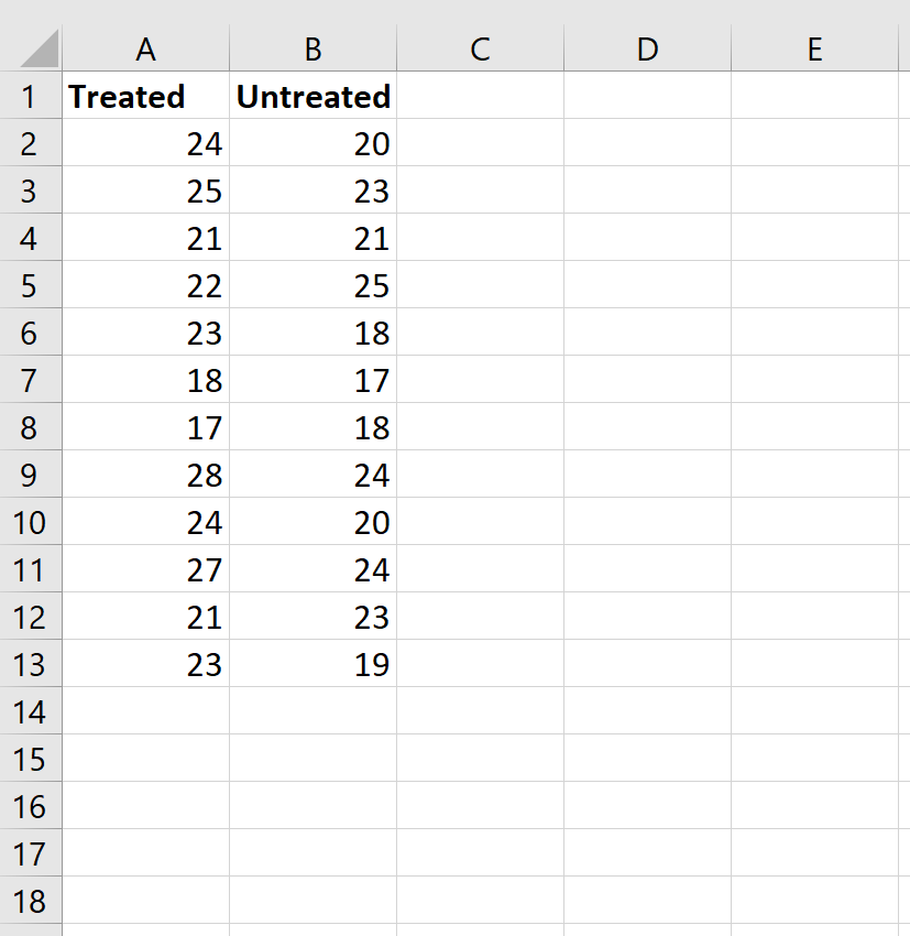
Шаг 1: Введите данные.
Введите данные следующим образом:
Шаг 2: Рассчитайте ранги для обеих групп.
Далее мы рассчитаем ранги для каждой группы. На следующем изображении показана формула, используемая для расчета ранга первого значения в группе обработанных:
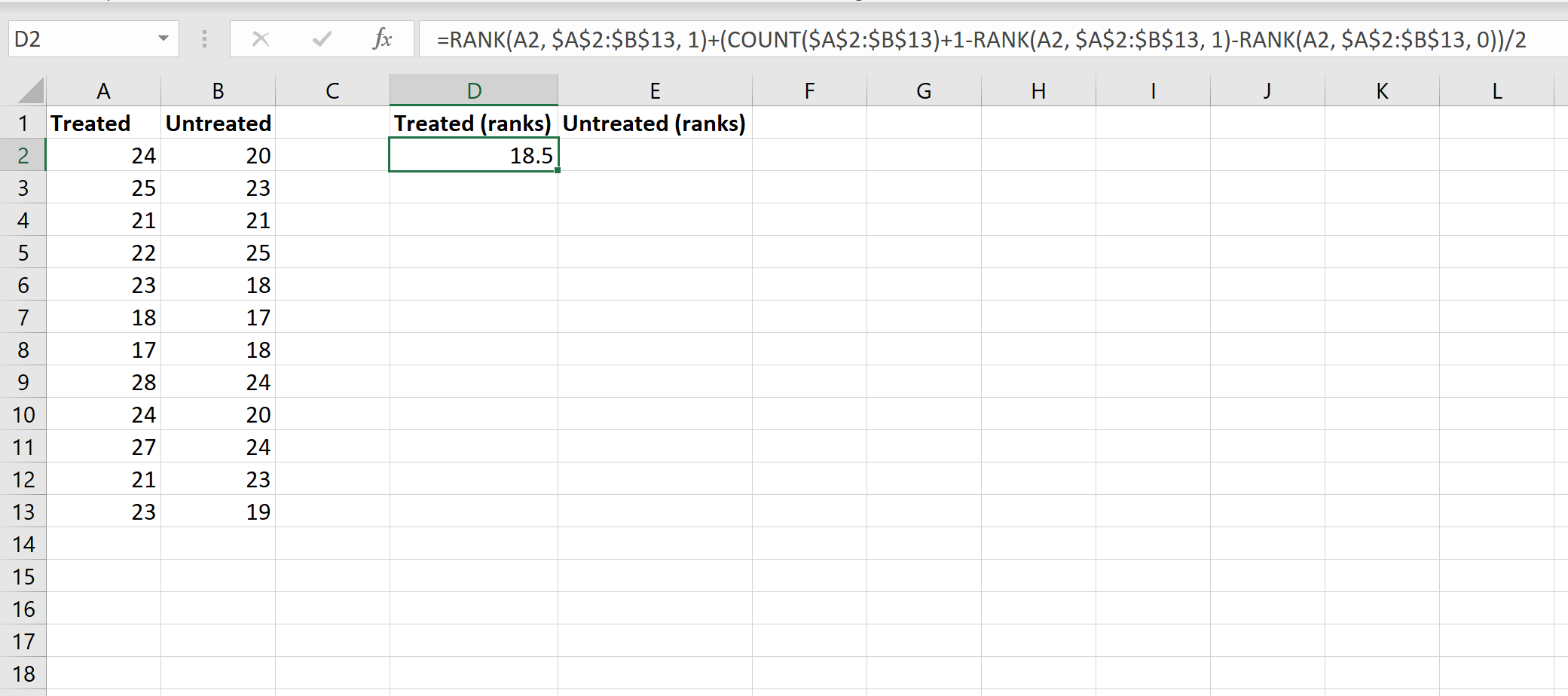
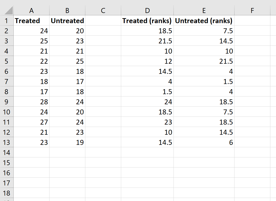
Хотя эта формула довольно сложна, вам нужно ввести ее только один раз. Затем вы можете просто перетащить формулу во все остальные ячейки, чтобы заполнить ранги:
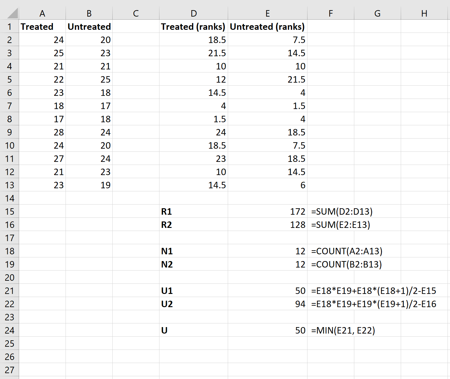
Шаг 3: Рассчитайте необходимые значения для тестовой статистики.
Затем мы будем использовать следующие формулы для расчета суммы рангов для каждой группы, размера выборки для каждой группы, статистики U-теста для каждой группы и общей статистики U-теста:
Шаг 4: Рассчитайте статистику теста z и соответствующее значение p.
Наконец, мы будем использовать следующие формулы для расчета статистики теста z и соответствующего значения p, чтобы определить, должны ли мы отклонить или не отклонить нулевую гипотезу:
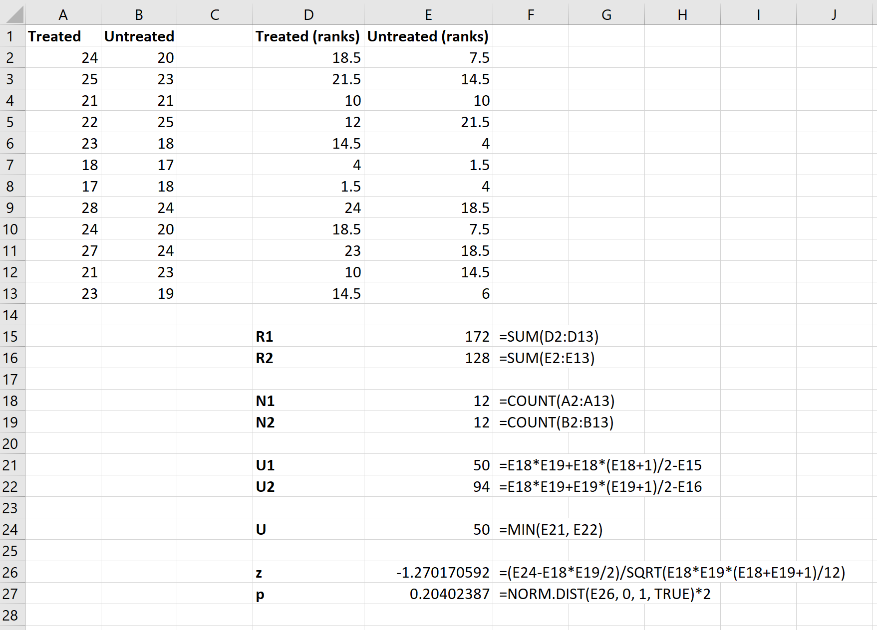
Нулевая гипотеза теста утверждает, что две группы имеют одинаковое среднее значение расхода топлива на галлон. Поскольку p-значение теста ( 0,20402387 ) не меньше нашего уровня значимости 0,05, мы не можем отвергнуть нулевую гипотезу.
У нас нет достаточных доказательств, чтобы сказать, что истинное среднее значение расхода на галлон отличается между двумя группами.
Содержание
- Как выполнить U-тест Манна-Уитни в Excel
- Критерий Манна-Уитни
- Пример расчета критерия Манна-Уитни
- Mann-Whitney test in Excel tutorial
- What is a Mann-Whitney test?
- Dataset for running a Mann-Whitney test in Excel
- Setting up a Mann-Whitney test on two independent samples
- Interpreting the results of a Mann Whitney test on two independent samples
- Mann-Whitney Test for Independent Samples
- Exact Test
- Simulation
- Confidence Interval of the Median
- Statistical Power and Sample Size
- 123 thoughts on “Mann-Whitney Test for Independent Samples”
Как выполнить U-тест Манна-Уитни в Excel

U-критерий Манна-Уитни (иногда называемый критерием суммы рангов Уилкоксона) используется для сравнения различий между двумя выборками, когда распределение выборки не является нормальным, а размеры выборки малы (n
Шаг 2: Рассчитайте ранги для обеих групп.
Далее мы рассчитаем ранги для каждой группы. На следующем изображении показана формула, используемая для расчета ранга первого значения в группе обработанных:
Хотя эта формула довольно сложна, вам нужно ввести ее только один раз. Затем вы можете просто перетащить формулу во все остальные ячейки, чтобы заполнить ранги:
Шаг 3: Рассчитайте необходимые значения для тестовой статистики.
Затем мы будем использовать следующие формулы для расчета суммы рангов для каждой группы, размера выборки для каждой группы, статистики U-теста для каждой группы и общей статистики U-теста:
Шаг 4: Рассчитайте статистику теста z и соответствующее значение p.
Наконец, мы будем использовать следующие формулы для расчета статистики теста z и соответствующего значения p, чтобы определить, должны ли мы отклонить или не отклонить нулевую гипотезу:
Нулевая гипотеза теста утверждает, что две группы имеют одинаковое среднее значение расхода топлива на галлон. Поскольку p-значение теста ( 0,20402387 ) не меньше нашего уровня значимости 0,05, мы не можем отвергнуть нулевую гипотезу.
У нас нет достаточных доказательств, чтобы сказать, что истинное среднее значение расхода на галлон отличается между двумя группами.
Источник
Критерий Манна-Уитни
Непараметрический критерий Манна-Уитни используется для сравнения двух независимых выборок. При этом совсем не важно, чтобы выборки были одинакового размера. Напомним, что все элементы из первой выборки сравниваются со всеми элементами второй выборки. Если какой-то элемент больше сравниваемого, то ему засчитывается 1 балл. Если элементы равны, то им засчитывается по 0,5 балла. Затем баллы элементов для каждой выборки суммируются, а меньшая полученная сумма является критерием – U-статистика. Если выборки не имеют существенных различий, то значение критерия должно быть больше критического значения для выборок соответствующего размера.
Примечание.
Здесь приведено очень упрощенное описание критерия Манна-Уитни, т.к. подразумевается, что Вы уже с ним знакомы.
Пример расчета критерия Манна-Уитни
У нас есть небольшой набор данных с эффективностью продаж двух продавцов:
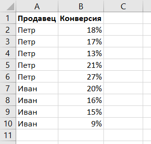
Мы хотим определить, какой из продавцов работает лучше, и выплатить лучшему продавцу повышенную премию. Сделаем это с помощью надстройки от office-menu.
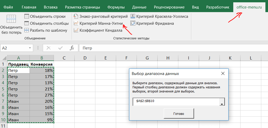
Перейдем на вкладку надстройки и кликнем на ленте пункт с нужным критерием, после чего будет предложено выбрать диапазон с данными для анализа. Диапазон выбирается без заголовков, первый столбец должен содержать наименование выборок, второй значения для них.
После клика по кнопке «Готово» откроется новая книга Excel с готовым расчетом и вспомогательной таблицей.
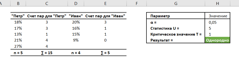
Из анализа видно, несмотря на то что продавец Иван хоть и имеет низкую конверсию в сравнении с Петром, это не говорит о том, что он работает хуже, а высокая конверсия Петра может быть выбросами в данных. Возможно на больших выборках результаты поменяются, но на текущем наборе говорить о существенных различиях нельзя.
Для того, чтобы использовать описанные в данной категории функции, скачайте и установите нашу надстройку.
Работа надстройки была успешно протестирована на версиях Excel: 2007, 2010 и 2013. В случае возникновения проблем с ее использованием, сообщайте Администрации сайта.
Источник
Mann-Whitney test in Excel tutorial
This tutorial will help you run and interpret a Mann-Whitney test on two independent samples in Excel using XLSTAT.
What is a Mann-Whitney test?
The Mann-Whitney test is a non parametric test that allows to compare two independent samples.
Three researchers, Mann, Whitney, and Wilcoxon, separately perfected a very similar non-parametric test which can determine if the samples may be considered identical or not on the basis of their ranks.
This test can only be used to study the relative positions of the samples. For example, if we generate a sample of 500 observations taken from an N(0,1) distribution and a sample from a distribution of 500 observations from an N(0,4) distribution, the Mann-Whitney test will find no difference between the samples.
The results proposed by XLSTAT are based on the U statistic of Mann-Whitney.
Dataset for running a Mann-Whitney test in Excel
The data are from [Fisher M. (1936), The Use of Multiple Measurements in Taxonomic Problems. Annals of Eugenics, 7, 179 -188] and correspond to 100 Iris flowers, described by four variables (sepal length, sepal width, petal length, petal width) and their species. The original dataset contains 150 flowers and 3 species, but we have isolated for this tutorials the observations belonging to the versicolor and virginica species. Our goal is to test if for the four variables, there is a clear difference between the two species.
The goal of this tutorial is to compare the two species with respect to the four variables independently.
Setting up a Mann-Whitney test on two independent samples
Once XLSTAT-Pro is activated, select the XLSTAT / Nonparametric tests / Comparison of two samples (Wilcoxon, Mann-Whitney, . ) command.

Once you’ve clicked the button, the dialog box appears. You can then select the data on the Excel sheet. Select the one column per variable option because, we have 4 columns of data and one column corresponding to the species identifiers. 
In the options tab, we suppose that the difference between samples is equal to 0. Note that exact p-value can be computed with XLSTAT. 
After you have clicked on the OK button, the results are displayed on a new Excel sheet (because the Sheet option has been selected for outputs).
Interpreting the results of a Mann Whitney test on two independent samples
The first results displayed are the statistics for the various samples. For each variable, we obtain a test result.
We can see that for the first variable, the null hypothesis of equality is rejected. We can consider that the sepal length is significantly different from one specie to the other.

Results for the other variables are also available in the output.
Not sure you chose the right test? This guide will let you know.
Источник
Mann-Whitney Test for Independent Samples
The Mann-Whitney U test is essentially an alternative form of the Wilcoxon Rank-Sum test for independent samples and is completely equivalent.
Define the following test statistics for samples 1 and 2 where n1 is the size of sample 1 and n2 is the size of sample 2, and R1 is the adjusted rank-sum for sample 1 and R2 is the adjusted rank-sum of sample 2. It doesn’t matter which sample is bigger.

As for the Wilcoxon version of the test, if the observed value of U is
Example 1: Repeat Example 1 of the Wilcoxon Rank Sum Test using the Mann-Whitney U test.
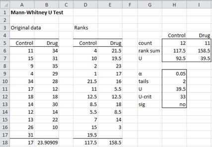
Figure 1 – Mann-Whitney U Test
Observation: Click here for proofs of Property 1 and 2.
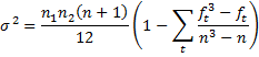
Property 3: Where there are a number of ties, the following revised version of the variance gives better results:
where n = n1 + n2, t varies over the set of tied ranks and ft is the number of times (i.e. frequency) the rank t appears. An equivalent formula is
Observation: A further complication is that it is often desirable to account for the fact that we are approximating a discrete distribution via a continuous one by applying a continuity correction. This is done by using a z-score of
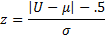
instead of the same formula without the .5 continuity correction factor.
Example 2: Repeat Example 2 of the Wilcoxon Rank Sum Test using the Mann-Whitney U test.
We show the results of the one-tailed test (without using a ties correction) is shown in Figure 2. Column W displays the formulas used in column T.
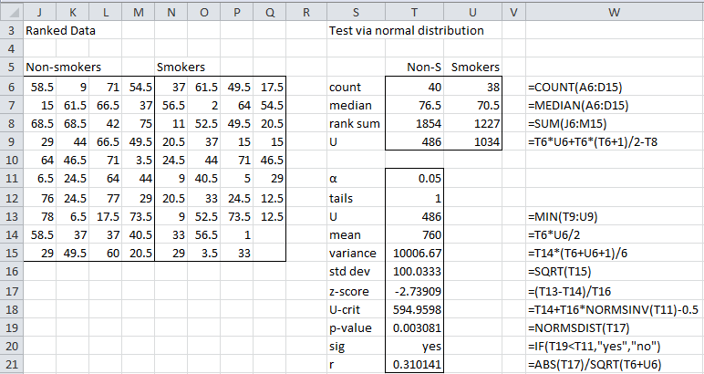
Figure 2 – Mann-Whitney U test using normal approximation
As can be seen in cell T19, the p-value for the one-tail test is the same as that found in Wilcoxon Example 2 using the Wilcoxon rank-sum test. Once again we reject the null hypothesis and conclude that non-smokers live significantly longer.
Observation: The effect size for the data using the Mann-Whitney test can be calculated in the same manner as for the Wilcoxon rank-sum test, namely

and the result will be the same, which for Example 2 is r = .31, as shown in cell T21.
There is another measure of effect size, namely

This represents the probability that a score randomly generated from population A will be bigger than a score randomly generated from population B, where A and B are the populations corresponding to the two samples and A corresponds to the sample with the higher value. The higher this value is the larger the effect.
Real Statistics Excel Functions: The following functions are provided in the Real Statistics Pack:
MANN(R1, R2) = U for the samples contained in ranges R1 and R2
MANN(R1, n) = U for the sample contained in the first n columns of range R1 and the sample consisting of the remaining columns in range R1. If the second argument is omitted it defaults to 1.
MWTEST(R1, R2, tails, ties, cont) = p-value of the Mann-Whitney U test for the samples contained in ranges R1 and R2 using the normal approximation. tails = 1 or 2 (default). If ties = TRUE (default) the ties correction factor is applied. If cont = TRUE (default) a continuity correction is applied.
Any empty or non-numeric cells in R1 or R2 are ignored.
Observation: For Example 2, we can use the Real Statistics MANN function to arrive at the value of 486 for U shown in cell T9 of Figure 2, namely =MANN(J6:M15,N6:Q15) = 486. Similarly, the p-value of 0.003081 in cell T19 can be calculated by =MWTEST(J6:M15,N6:Q15,1,FALSE,TRUE).
Observation: Note that the z-score and the effect size r can be calculated using the Real Statistics function MWTEST as follows:
z-score = NORM.S.INV(MWTEST(R1, R2))
r = NORM.S.INV(MWTEST(R1, R2))/SQRT(COUNT(R1)+COUNT(R2))
Observation: The results of analysis for Example 2 can be summarized as follows: The life expectancy of non-smokers (Mdn = 76.5) is significantly higher than that of smokers (Mdn = 70.5), U = 486, z = -2.74, p = .0038
Of course, you can also use a two-tailed test with ties correction, as we will demonstrate shortly.
Real Statistics Function: The following function is provided in the Real Statistics Pack and returns output consisting of the U-stat, z-stat, r effect size and the three types of p-values (the normal approximation, exact test and simulation).
MW_TEST(R1, R2, lab, tails, ties, cont, exact, iter): returns a column array with the output described above for the samples contained in ranges R1 and R2. tails = 1 or 2 (default). For the normal approximation, if ties = TRUE (default) the ties correction factor is applied; if cont = TRUE (default) a continuity correction is applied; if exact = TRUE (default FALSE) then the p-value of the exact test is output and if iter ≠ 0 then the p-value of the simulation version of the test is output where the simulation consists of iter samples (default 10,000). If lab = TRUE (default FALSE) then an extra column of labels is appended to the output.
Any empty or non-numeric cells in R1 or R2 are ignored. See Mann-Whitney Exact Test and Mann-Whitney Simulation for more information about the exact test and simulation p-values.
Figure 3 displays the output from =MW_TEST(A6:A17,B6:B17,TRUE) for Example 2.
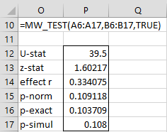
Figure 3 – Output from MW_TEST
Observation: Even if the argument is set to FALSE, the p-value of the exact test will be produced provided both samples have fewer than 800 elements and the smaller sample has at most 300 elements.
Real Statistics Data Analysis Tool: The Real Statistics Resource Pack also provides a data analysis tool that performs the Mann-Whitney test for independent samples, automatically calculating the medians, rank sums, U test statistic, z-score, p-values and effect size r.
For example, to perform the analysis in Example 1, press Ctrl-m and choose the T Test and Non-parametric Equivalents data analysis tool from the menu that appears (or from the Misc tab if using the Multipage user interface). The dialog box shown in Figure 4 now appears.

Figure 4 – Dialog box for Real Statistics Mann-Whitney Test
Enter A5:B17 as the Input Range 1 (alternatively insert A5:A17 in Input Range 1 and B5:B17 in Input Range 2), click on Column headings included with data, choose the Two independent samples and Non-parametric options and click on the OK button. Keep the default of 0 for Hypothetical Mean/Median and .05 for Alpha (although these values are not used) For this version of the test, we check Use continuity correction, Include exact test and Include table lookup but we leave the Use ties correction option unchecked.
The output is shown in Figure 5.
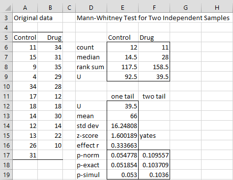
Figure 5 – Mann-Whitney test data analysis tool output
Note that both the one-tail and two-tail tests are displayed. Also, three versions of the test are shown: the test using the normal approximation (range E17:F17), the test using the exact test (range E18:F18) and the simulation test (range E19:F19). The fact that the “Yates” continuity correction factor is used is noted in cell F15.
If we check the Use Ties correction option in Figure 4 we would obtain the output shown in Figure 6.
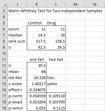
Figure 6 – Mann-Whitney test with ties correction
In this case the ties correction of Property 3 is applied to the normal approximation. As you can see there is very little difference between the outputs shown in Figure 5 and 6.
Note too that the ties correction (as well as the continuity correction) only applies to the normal approximation. The ties and continuity corrections are not applied to the exact and simulation versions of the test. The difference in the simulation p-values (row 19) in Figure 5 and 6 is due to the randomness of the simulations and not the ties correction.
Real Statistics Function: The Real Statistics Pack provides the following function to calculate the ties correction used in the data analysis tool.
TiesCorrection(R1, R2, type) = ties correction value for the data in range R1 and optionally range R2, where type = 0: one sample, type = 1: paired sample and type = 2: independent samples
For the Mann-Whitney test type = 2. The ties correction is used in the calculation of the standard deviation (cell U15 of Figure 6) as follows
Exact Test
Click here for a description of the exact version of the Mann-Whitney Test using the permutation function.
Simulation
Click here for a description of how to use simulation to determine the p-value for the Mann-Whitney test. This approach takes ties into account.
Confidence Interval of the Median
Click here for a description of how to calculate a confidence interval of the median based on the Mann-Whitney Test.
Statistical Power and Sample Size
Click here for a description of how to calculate the statistical power or minimum sample size required for the Mann-Whitney Test.
123 thoughts on “Mann-Whitney Test for Independent Samples”
I have determined that my data is not normally distributed, therefore I need to perform a non-parametric test. I am doing a project where I need to compare patient characteristics to literature. In some articles, I only have the median or only the mean of the group. Using the real statistics toolpack, I have managed to find the p-value for the characteristics where I only have the median. I was wondering how I could do the Mann-Whitney test if I want to compare my sample’s mean to a mean found in an article.
Nicole,
Do you have the data or just the two means?
Charles
I have my data which consists of 48 measurements (example patient age) for which I can have its mean, median, standard deviation,etc… In some articles for their patients, they provide only the median, therefore I used the Wilcoxon Signed-Rank Test for a Single Sample to compare their median to my median (is this correct?). But in another articles, I only have the mean for the group and I don’t know how to go about it. Thank you!
Is the data that you have reasonably symmetric?
Charles
I drew the histogram for age and weight of my patients and it is not very symmetrical. I am required to use the U Mann Whitney test to do this.
Sorry Nicole, but I don’t know how to test whether a data sample comes from a population with a given mean using the Mann Whitney test or the Wilcoxon Signed Ranks test. When the data is symmetric, the mean and median are the same, and so assuming this is also true of the population from which the sample is drawn, then the Wilcoxon Signed Ranks test could be useful.
Charles
Hi Charles, hope you’ve been well!
I’m using the MW U Test for Likert Scale Data (5-point),
I just wanted to ask, if Sample 1 got a higher mean rank than sample 2, that means that Sample 1’s Likert scores has a higher average than sample 2. But for that test, the Z-score yielded a negative value which also means that it is below the mean distribution.
Wouldn’t that be conflicting? If not, then what other importance of Z-score that I am missing?
Thank you in advance.
Ken,
If you send me an Excel file with your data and test results, it will be easier for me to answer your question.
Charles
Hi Charles,
In the operationalization of Mann Whitney U test, after computing U1 and U2, why do we choose the minimum of them as U statistic?
Is there any logic or statistical reasons for it? Please elaborate.
Hello Anand,
I don’t know for sure, but it is probably related to consistently using the same set of critical values (i.e. the same tail of the distribution).
Charles
Hello, very good information.
I wanted to ask you I have to do a statistical project about U-Mann Whitney/ANOV-systolic Pressure(mmHg) for the first 20 men and 15 first women. I have no idea how to start my work, but if you can help me with this work, I would be very happy. In addition to that, I need to be guided by Mario Triola’s book Edition 10 on page 786-787.
If you could please help me I would be grateful.
What the teacher requires for this work is :
Introduction/Objective
Data collection or Data provide
The topic of the projects -definitions, Hypotheses, formulas, calculations, tables, graphs, etc.
Thank you!!
Can anyone help me with that?
Yazmin,
I am happy to answer specific questions, but you need to do the homework assignment yourself.
Charles
Thank you for all your help with this real stats package. My queries might be too simple so apologies in advance. I have two independent groups of businesses: Group 1 low use of financial budgets and Group 2 high use of financial budgets. I want to show that Group 2 of businesses with high use of budgets have higher revenue. This was a survey based (likert scale) research not experimental.
a) which of the test statistic would you recommend I report? I have read this should be P exact. I have not applied continuity here.
b) Is there a particular rule as to which of the two independent group’s data I should put into input 1 field in your stats package? Should be it be group 1 by natural order? I don’t have a control group as such as I conducted survey research.
c) The reason I ask Question B above is when I switch it around and put group 2 data in input 1, it makes no difference to the test statistics reported in the statistics table. How does the real stats know which group is being compared to which? How do I know that my hypothesis that group 2 has high revenue is proven?
I hope that makes sense and thank you for your help!
Hello Saad,
a) If you don’t have any ties (or few ties), the exact test is probably the right choice. If the sample size is not too small then the normal approaximation is probably best if ties are an issue.
b) The order should not matter
c) With two groups, the two groups are compared to each other. If you get a significant result, then the group whose sample has the higher revenue is the group whose population revenue will be higher.
Charles
Источник
Перейти к содержимому
Онлайн калькулятор непараметрического критерия U Манна-Уитни позволяет получить расчет сразу на сайте. Итоговое описание состоит из таблиц, графиков и текстовых выводов. Его можно сказать в формате Word, а таблицы в Excel.
Читать далее Онлайн расчет критерия U-Манна-Уитни
В данном видео описан пошаговый алгоритм расчета критерия U Манна-Уитни в программе SPSS.
Читать далее [Видео] Алгоритм расчета критерия U Манна-Уитни в SPSS
В этом обучающем видео представлена интерпретация результатов расчета критерия U Манна-Уитни в программе SPSS.
Читать далее [Видео] Интерпретация результатов расчета критерия U Манна Уитни в SPSS
В данной таблице представлены критические значения критерия U-Манна-Уитни для уровня значимости 0,05 и уровня значимости 0,01.
Читать далее Таблица критических значений критерия U-Манна-Уитни
Для того, чтобы рассчитать непараметрический критерий U Манна-Уитни для независимых выборок используя статистически пакет SPSS необходимо сделать следующий шаги:
Читать далее Расчет критерия U Манна-Уитни в SPSS
Непараметрический критерий U Манна-Уитни применяется для сравнения средних значений двух независимых выборок.
Условия применения:
Читать далее Непараметрический критерий U Манна-Уитни
The Mann-Whitney U test is essentially an alternative form of the Wilcoxon Rank-Sum test for independent samples and is completely equivalent.
Define the following test statistics for samples 1 and 2 where n1 is the size of sample 1 and n2 is the size of sample 2, and R1 is the adjusted rank-sum for sample 1 and R2 is the adjusted rank-sum of sample 2. It doesn’t matter which sample is bigger.
![]()
![]()
As for the Wilcoxon version of the test, if the observed value of U is < Ucrit then the test is significant (at the α level), i.e. we reject the null hypothesis. The values of Ucrit for α = .05 (two-tailed) are given in the Mann-Whitney Tables.
Example 1: Repeat Example 1 of the Wilcoxon Rank Sum Test using the Mann-Whitney U test.
Figure 1 – Mann-Whitney U Test
Since R1 = 117.5 and R2 = 158.5, we can calculate U1 and U2 to get U = 39.5. Next we look up in the Mann-Whitney Tables for n1 = 12 and n2 = 11 to get Ucrit = 33. Since 33 < 39.5, we cannot reject the null hypothesis at α = .05 level of significance.
Property 1:
![]()
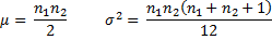
Property 2: For n1 and n2 large enough the U statistic is approximately normal N(μ, σ) where
![]()
Observation: Click here for proofs of Property 1 and 2.
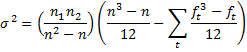
Property 3: Where there are a number of ties, the following revised version of the variance gives better results:
where n = n1 + n2, t varies over the set of tied ranks and ft is the number of times (i.e. frequency) the rank t appears. An equivalent formula is
Observation: A further complication is that it is often desirable to account for the fact that we are approximating a discrete distribution via a continuous one by applying a continuity correction. This is done by using a z-score of
![]()
instead of the same formula without the .5 continuity correction factor.
Example 2: Repeat Example 2 of the Wilcoxon Rank Sum Test using the Mann-Whitney U test.
We show the results of the one-tailed test (without using a ties correction) is shown in Figure 2. Column W displays the formulas used in column T.
Figure 2 – Mann-Whitney U test using normal approximation
As can be seen in cell T19, the p-value for the one-tail test is the same as that found in Wilcoxon Example 2 using the Wilcoxon rank-sum test. Once again we reject the null hypothesis and conclude that non-smokers live significantly longer.
Observation: The effect size for the data using the Mann-Whitney test can be calculated in the same manner as for the Wilcoxon rank-sum test, namely
![]()
and the result will be the same, which for Example 2 is r = .31, as shown in cell T21.
There is another measure of effect size, namely
![]()
This represents the probability that a score randomly generated from population A will be bigger than a score randomly generated from population B, where A and B are the populations corresponding to the two samples and A corresponds to the sample with the higher value. The higher this value is the larger the effect.
Real Statistics Excel Functions: The following functions are provided in the Real Statistics Pack:
MANN(R1, R2) = U for the samples contained in ranges R1 and R2
MANN(R1, n) = U for the sample contained in the first n columns of range R1 and the sample consisting of the remaining columns in range R1. If the second argument is omitted it defaults to 1.
MWTEST(R1, R2, tails, ties, cont) = p-value of the Mann-Whitney U test for the samples contained in ranges R1 and R2 using the normal approximation. tails = 1 or 2 (default). If ties = TRUE (default) the ties correction factor is applied. If cont = TRUE (default) a continuity correction is applied.
Any empty or non-numeric cells in R1 or R2 are ignored.
Observation: For Example 2, we can use the Real Statistics MANN function to arrive at the value of 486 for U shown in cell T9 of Figure 2, namely =MANN(J6:M15,N6:Q15) = 486. Similarly, the p-value of 0.003081 in cell T19 can be calculated by =MWTEST(J6:M15,N6:Q15,1,FALSE,TRUE).
Observation: Note that the z-score and the effect size r can be calculated using the Real Statistics function MWTEST as follows:
z-score = NORM.S.INV(MWTEST(R1, R2))
r = NORM.S.INV(MWTEST(R1, R2))/SQRT(COUNT(R1)+COUNT(R2))
Observation: The results of analysis for Example 2 can be summarized as follows: The life expectancy of non-smokers (Mdn = 76.5) is significantly higher than that of smokers (Mdn = 70.5), U = 486, z = -2.74, p = .0038 < .05, r = .31, based on a one-tailed test Mann-Whitney test with continuity correction, but no correction for ties.
Of course, you can also use a two-tailed test with ties correction, as we will demonstrate shortly.
Real Statistics Function: The following function is provided in the Real Statistics Pack and returns output consisting of the U-stat, z-stat, r effect size and the three types of p-values (the normal approximation, exact test and simulation).
MW_TEST(R1, R2, lab, tails, ties, cont, exact, iter): returns a column array with the output described above for the samples contained in ranges R1 and R2. tails = 1 or 2 (default). For the normal approximation, if ties = TRUE (default) the ties correction factor is applied; if cont = TRUE (default) a continuity correction is applied; if exact = TRUE (default FALSE) then the p-value of the exact test is output and if iter ≠ 0 then the p-value of the simulation version of the test is output where the simulation consists of iter samples (default 10,000). If lab = TRUE (default FALSE) then an extra column of labels is appended to the output.
Any empty or non-numeric cells in R1 or R2 are ignored. See Mann-Whitney Exact Test and Mann-Whitney Simulation for more information about the exact test and simulation p-values.
Figure 3 displays the output from =MW_TEST(A6:A17,B6:B17,TRUE) for Example 2.
Figure 3 – Output from MW_TEST
Observation: Even if the argument is set to FALSE, the p-value of the exact test will be produced provided both samples have fewer than 800 elements and the smaller sample has at most 300 elements.
Real Statistics Data Analysis Tool: The Real Statistics Resource Pack also provides a data analysis tool that performs the Mann-Whitney test for independent samples, automatically calculating the medians, rank sums, U test statistic, z-score, p-values and effect size r.
For example, to perform the analysis in Example 1, press Ctrl-m and choose the T Test and Non-parametric Equivalents data analysis tool from the menu that appears (or from the Misc tab if using the Multipage user interface). The dialog box shown in Figure 4 now appears.
Figure 4 – Dialog box for Real Statistics Mann-Whitney Test
Enter A5:B17 as the Input Range 1 (alternatively insert A5:A17 in Input Range 1 and B5:B17 in Input Range 2), click on Column headings included with data, choose the Two independent samples and Non-parametric options and click on the OK button. Keep the default of 0 for Hypothetical Mean/Median and .05 for Alpha (although these values are not used) For this version of the test, we check Use continuity correction, Include exact test and Include table lookup but we leave the Use ties correction option unchecked.
The output is shown in Figure 5.
Figure 5 – Mann-Whitney test data analysis tool output
Note that both the one-tail and two-tail tests are displayed. Also, three versions of the test are shown: the test using the normal approximation (range E17:F17), the test using the exact test (range E18:F18) and the simulation test (range E19:F19). The fact that the “Yates” continuity correction factor is used is noted in cell F15.
If we check the Use Ties correction option in Figure 4 we would obtain the output shown in Figure 6.
Figure 6 – Mann-Whitney test with ties correction
In this case the ties correction of Property 3 is applied to the normal approximation. As you can see there is very little difference between the outputs shown in Figure 5 and 6.
Note too that the ties correction (as well as the continuity correction) only applies to the normal approximation. The ties and continuity corrections are not applied to the exact and simulation versions of the test. The difference in the simulation p-values (row 19) in Figure 5 and 6 is due to the randomness of the simulations and not the ties correction.
Real Statistics Function: The Real Statistics Pack provides the following function to calculate the ties correction used in the data analysis tool.
TiesCorrection(R1, R2, type) = ties correction value for the data in range R1 and optionally range R2, where type = 0: one sample, type = 1: paired sample and type = 2: independent samples
For the Mann-Whitney test type = 2. The ties correction is used in the calculation of the standard deviation (cell U15 of Figure 6) as follows
=SQRT(K13*(K6+L6+1)/6*(1-TiesCorrection(A6:A17,B6:B17,2)/ ((K6+L6)^3-K6-L6)))
Exact Test
Click here for a description of the exact version of the Mann-Whitney Test using the permutation function.
Simulation
Click here for a description of how to use simulation to determine the p-value for the Mann-Whitney test. This approach takes ties into account.
Confidence Interval of the Median
Click here for a description of how to calculate a confidence interval of the median based on the Mann-Whitney Test.
Statistical Power and Sample Size
Click here for a description of how to calculate the statistical power or minimum sample size required for the Mann-Whitney Test.
This tutorial will help you run and interpret a Mann-Whitney test on two independent samples in Excel using XLSTAT.
What is a Mann-Whitney test?
The Mann-Whitney test is a non parametric test that allows to compare two independent samples.
Three researchers, Mann, Whitney, and Wilcoxon, separately perfected a very similar non-parametric test which can determine if the samples may be considered identical or not on the basis of their ranks.
This test can only be used to study the relative positions of the samples. For example, if we generate a sample of 500 observations taken from an N(0,1) distribution and a sample from a distribution of 500 observations from an N(0,4) distribution, the Mann-Whitney test will find no difference between the samples.
The results proposed by XLSTAT are based on the U statistic of Mann-Whitney.
Dataset for running a Mann-Whitney test in Excel
The data are from [Fisher M. (1936), The Use of Multiple Measurements in Taxonomic Problems. Annals of Eugenics, 7, 179 -188] and correspond to 100 Iris flowers, described by four variables (sepal length, sepal width, petal length, petal width) and their species. The original dataset contains 150 flowers and 3 species, but we have isolated for this tutorials the observations belonging to the versicolor and virginica species. Our goal is to test if for the four variables, there is a clear difference between the two species.
The goal of this tutorial is to compare the two species with respect to the four variables independently.
Setting up a Mann-Whitney test on two independent samples
Once XLSTAT-Pro is activated, select the XLSTAT / Nonparametric tests / Comparison of two samples (Wilcoxon, Mann-Whitney, …) command.
Once you’ve clicked the button, the dialog box appears. You can then select the data on the Excel sheet. Select the one column per variable option because, we have 4 columns of data and one column corresponding to the species identifiers.
In the options tab, we suppose that the difference between samples is equal to 0. Note that exact p-value can be computed with XLSTAT.
After you have clicked on the OK button, the results are displayed on a new Excel sheet (because the Sheet option has been selected for outputs).
Interpreting the results of a Mann Whitney test on two independent samples
The first results displayed are the statistics for the various samples. For each variable, we obtain a test result.
We can see that for the first variable, the null hypothesis of equality is rejected. We can consider that the sepal length is significantly different from one specie to the other.
Results for the other variables are also available in the output.
Not sure you chose the right test? This guide will let you know.
Was this article useful?
- Yes
- No
Mann-Whitney Test in Excel Using QI Macros
When to Use the Mann-Whitney Test
A Mann-Whitney test (equivalent to Wilcoxon Rank Sum Test) compares the differences between two independent samples to determine if they differ in location.
Use Mann-Whitney or Wilcoxon Rank Sum tests instead of Mood’s Median Test, as they provide more accurate results.
Note: Excel does not do statistical tests of non-normal (i.e., not «bell shaped») data. QI Macros, adds this functionality with a set of of non-parametric test templates.
Mann-Whitney Example
A professor wants to compare the grades of students who attended live lectures vs video-taped lectures. Scores of students attending video lectures is in column A; live lectures in column B.
To conduct a test using QI Macros he will:
- Click on the QI Macros menu > Stat Templates > Mann Whitney
- Input the data for Sample 1 (Video Taped Lectures) into column A and the data for Sample 2 (Live Lectures) into column B.
- QI Macros will perform the calculations and display the results in columns C:G.
- QI Macros will also interpret the results for you. Cell F7 indicates that we cannot reject the null hypothesis (accept the null hypothesis):
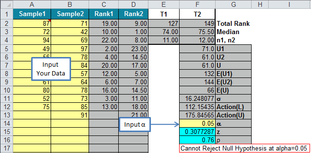
Interpreting the Mann Whitney Test Results: Since p (0.758) is greater than alpha (0.05) we cannot reject the null hypothesis (accept the null hypothesis) that video instruction is as good as live instruction.
Tip: As you enter additional rows of data in columns A and B, the formulas in columns C and D should be automatically extended. If they do not extend, you can extend them yourself using copy and paste.
NOTE: If p < 0.05 Reject the Null Hypothesis.
Why Choose QI Macros Statistical Software for Excel?
![]()
Easy to Use
- Works Right in Excel
- Interprets p-values for You
- Accurate No-Worry Results
- Free Training Anytime
![]()
Proven and Trusted
- 100,000 Users in 80 Countries
- Celebrating 20th Anniversary
- Five Star CNET Rating — Virus Free
![]()
Affordable
- Only $349 USD
Quantity Discounts Available - No annual fees
- Free Technical Support
-

-
May 31 2012, 09:25
- Литература
- Общество
- Психология
- Cancel
Сделал черновой вариант расчета U-критерия Манна-Уитни в MS Excel. Вроде работает правильно, но я особо не проверял. Да, и в этом варианте нет поправки на связки (повторяющиеся наблюдения). Будет корректно работать при n1 и n2 >20 и минимальном количестве повторяющихся наблюдений.
Обновленная версия реализации в MS Excel — форму отчета приблизил к форме отчета в SPSS.
См. также Полезные книги по математико-статистической обработке данных психологического исследования.
Originally published at В поиске предельных смыслов. You can comment here or there.