
Автор:
Robert Simon
Дата создания:
18 Июнь 2021
Дата обновления:
10 Апрель 2023
Содержание
- Шаг 1
- Шаг 2
- Шаг 3
- Шаг 4

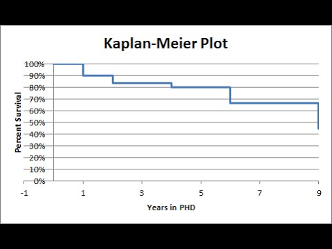
Диаграммы выживаемости Каплана-Мейера оценивают показатели выживаемости и настойчивость населения. Вы можете создать диаграмму Каплана-Мейера в Microsoft Excel. Организуйте свои данные для отображения правильной информации, создайте вычисляемый столбец для оценки выживаемости и график для отображения этой информации. Настройте свою графику, выбрав цветовую схему, стиль шрифта и эффекты. Поделитесь своими данными, распечатав, отправив по почте или вставив изображение в презентацию.
Шаг 1
Откройте электронную таблицу Excel, содержащую данные о вашей выживаемости. Поместите свой период времени в столбец A, популяцию в столбец B и количество выживших в столбце C. Пометьте все столбцы описательными заголовками в первой строке.
Шаг 2
Вычислите оценку Каплана-Мейера в столбце D, разделив количество выживших на популяцию, а затем умножив на предыдущие оценки. Например, введите выражение «= (C2 / B2)» без кавычек для первой записи, «= (C2 / B2)(C3 / B3) «для второй записи и» = (C2 / B2)(C3 / B3) * (C4 / B4) «для третьей записи. Завершите выражения и пометьте столбец.
Шаг 3
Выберите столбец Каплана-Мейера и щелкните вкладку «Вставка» на ленте вверху экрана. Щелкните инструмент «Линия» диаграммы и выберите первую опцию в верхнем левом углу. Щелкните вкладку «Макет» на ленте, выберите параметр «Выбрать данные», нажмите «Изменить» под меткой горизонтальной оси «Категория» и выберите столбец A в текстовом поле «Диапазон диапазона меток». ось».
Настройте диаграмму выживаемости Каплана-Мейера, выбрав вкладки «Макет» и «Презентация» на ленте. Измените цветовую схему в области «Стили графики» на вкладке «Дизайн». Добавьте метки осей, легенды и заголовки для диаграммы на вкладке «Презентация».
This tutorial will show you how to set up and interpret a Kaplan-Meier analysis in Excel including group comparison using the XLSTAT software.
Dataset to run a Kaplan-Meier analysis
The data have been obtained in [Gehan E.A. (1965). A generalized Wilcoxon test for comparing arbitrarily singly-censored samples. Biometrika, 52, pp 203—223] and represent a randomized clinical trial investigating the effect of the drug 6-mercaptopurine on remission times (in weeks) of acute leukemia patients.
Goal of this Kaplan-Meier analysis
Our goal is to determine if and how the drug influences the survival time, by comparing the survival curves for two groups of 21 patients, the first being treated, and the second being a control group. All 21 patients of the control group were observed to have a recurrence of their leukemia. Only 9 of the 6-MP patients had an observed recurrence time, while the 12 others were censored.
Setting up a Kaplan-Meier analysis
-
Open XLSTAT
-
In the ribbon, select XLSTAT > Survival analysis > Kaplan-Meier analysis
-
Once you’ve clicked on the button, the Kaplan-Meier analysis box will appear. Select the data on the Excel sheet. The Time data corresponds to the durations when the patients either relapsed or were censored. The Status indicator describes whether a patient relapsed (event code=1) or was censored (censored code = 0) at a given time.

-
In the Data options tab, activate the By group analysis and select the group information in the data field. Thus XLSTAT will take into account the information whether the patient belongs to the control or the treated group. Activate the Compare option so that the comparison tests are computed. The Filter option allows you to select precisely the groups on which you wish to perform the analysis.
-
In the Charts tab, activate the charts you wish to display, and choose the symbol you want to use to represent Censored data.
-
The computations begin once you have clicked on OK. The results will then be displayed on a new Excel sheet.
Interpreting the results of a Kaplan-Meier analysis
The first table displays a summary of the data for each group:

Then XLSTAT displays results specific to each group. It starts with the Control group.
First, the Kaplan-Meier table is displayed. It contains the results of the Kaplan-Meier analysis with several key indicators such as the Survival distribution function.

The next tables give the mean and median survival time and the respective confidence intervals.

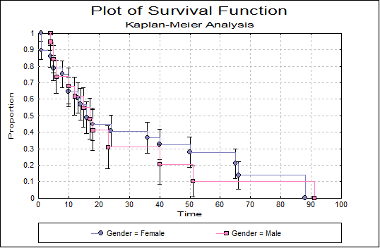
Then, we can visualize several curves, including the survival distribution function (SDF, or survivor function, or reliability function), bounded by the confidence intervals.

Next, the same series of results is displayed for the Drug 6-MP group.

The following results contain some values that are missing because they could not be computed.
We notice that the median survival time is a lot lower for the control group than for the 6-MP group (8.667 vs 21.943).

In the SDF, circles identify the censored data.

Then, we can compare the two groups. First, a series of tests is displayed in a table (Log-rank, Wilcoxon, Tarone-Ware). From the results we can see that the difference between the two survivor functions is very significant.

Last, the comparison of the two survival curves allows us to conclude to confirm that the drug significantly improves survival time of patients.

Was this article useful?
- Yes
- No
The goal of the Kaplan-Meier procedure is to create an estimator of the survival function based on empirical data, taking censoring into account.
Topics:
- Overview
- Survival Curve
- Standard Error and Confidence Intervals
- Hazard Function
- Log-Rank Test for Comparing Two Samples
- Alternative Tests for the Comparisons of Two Samples
- Hazard Ratio
- Real Statistics Capabilities
For those with a calculus background, you can also see the proofs of some of the properties described on the above webpages at
- Kaplan-Meier Theory
QI Macros has Three Ready-Made Kaplan-Meir Step Plot Options
Why it Matters: Kaplan-Meier Step Plots are used in health care to show survival rates over time for various protocols and treatments.
QI Macros Kaplan-Meier Step Plot Templates
- 1. Kaplan Meier Plot — One Group
- 2. Kaplan Meier for Two Groups
- 3. Step Plot Template
Kaplan-Meier Plot One Group
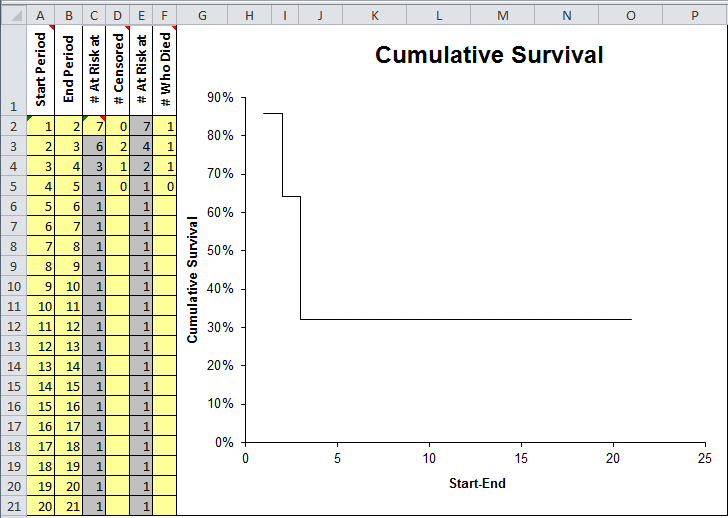
Data entry fields are shaded in yellow:
- Start Period (Could be a date or number)
- End Period (Could be a date or number)
- # At Risk at Start of the Period
- # Censored (Number removed from the study for various reasons)
- # At Risk at End
- # Who Died
The Y axis shows the cumulative survival rate. Cumulative survival rate may level off at the end of the study because patient survival is no longer tracked.
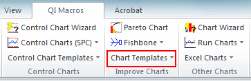
The Kaplan-Meir Step Plot is one of many charts and tools included in QI Macros add-in for Excel.
QI Macros adds a new tab to Excel’s menu, making it easy to find and open any chart template you need.
Other Charts in QI Macros Add-in for Excel
The UNISTAT statistics add-in extends Excel with Kaplan-Meier Analysis capabilities.
For further information visit UNISTAT User’s Guide section 9.4.2. Kaplan-Meier Analysis.
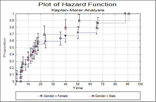
Here we provide a sample output from the UNISTAT Excel statistics add-in for data analysis.
Kaplan-Meier Analysis
Product Limit Survival Table
Factor variable: Gender = Female
Time Variable: Survival time
Censor Variable: Status
Number of Cases Censored: 7 ( 24.1%)
Valid Number of Cases: 29, 19 Omitted
| Time | Status | Number Entering | Number Terminating | Cumulative Proportion Surviving | Standard Error of Cumulative Surviving | Lower 95% of Cumulative Surviving | Upper 95% of Cumulative Surviving | Cumulative Proportion Terminating |
|---|---|---|---|---|---|---|---|---|
| 1 | 1 | 28 | 1 | * | * | * | * | * |
| 1 | 1 | 27 | 2 | * | * | * | * | * |
| 1 | 1 | 26 | 3 | 0.8966 | 0.0566 | 0.7126 | 0.9654 | 0.1034 |
| 3 | 0 | 25 | 3 | * | * | * | * | * |
| 4 | 1 | 24 | 4 | 0.8607 | 0.0647 | 0.6701 | 0.9453 | 0.1393 |
| 5 | 1 | 23 | 5 | * | * | * | * | * |
| 5 | 1 | 22 | 6 | 0.7890 | 0.0766 | 0.5891 | 0.8993 | 0.2110 |
| 8 | 1 | 21 | 7 | 0.7531 | 0.0811 | 0.5505 | 0.8740 | 0.2469 |
| 10 | 1 | 20 | 8 | * | * | * | * | * |
| 10 | 1 | 19 | 9 | * | * | * | * | * |
| 10 | 1 | 18 | 10 | 0.6455 | 0.0902 | 0.4411 | 0.7913 | 0.3545 |
| 10 | 0 | 17 | 10 | * | * | * | * | * |
| 13 | 1 | 16 | 11 | 0.6075 | 0.0926 | 0.4036 | 0.7606 | 0.3925 |
| 14 | 1 | 15 | 12 | 0.5696 | 0.0942 | 0.3673 | 0.7288 | 0.4304 |
| 15 | 0 | 14 | 12 | * | * | * | * | * |
| 16 | 1 | 13 | 13 | * | * | * | * | * |
| 16 | 1 | 12 | 14 | 0.4882 | 0.0968 | 0.2915 | 0.6590 | 0.5118 |
| 18 | 1 | 11 | 15 | 0.4475 | 0.0969 | 0.2559 | 0.6223 | 0.5525 |
| 24 | 1 | 10 | 16 | 0.4068 | 0.0962 | 0.2218 | 0.5844 | 0.5932 |
| 36 | 1 | 9 | 17 | 0.3662 | 0.0948 | 0.1892 | 0.5454 | 0.6338 |
| 40 | 1 | 8 | 18 | 0.3255 | 0.0926 | 0.1581 | 0.5051 | 0.6745 |
| 40 | 0 | 7 | 18 | * | * | * | * | * |
| 50 | 1 | 6 | 19 | 0.2790 | 0.0903 | 0.1227 | 0.4599 | 0.7210 |
| 52 | 0 | 5 | 19 | * | * | * | * | * |
| 56 | 0 | 4 | 19 | * | * | * | * | * |
| 65 | 1 | 3 | 20 | 0.2092 | 0.0907 | 0.0676 | 0.4031 | 0.7908 |
| 66 | 1 | 2 | 21 | 0.1395 | 0.0831 | 0.0284 | 0.3365 | 0.8605 |
| 76 | 0 | 1 | 21 | * | * | * | * | * |
| 88 | 1 | 0 | 22 | 0.0000 | 0.0000 | * | * | 1.0000 |
| Time | Standard Error of Cumulative Terminating | Lower 95% of Cumulative Terminating | Upper 95% of Cumulative Terminating | |||||
| 1 | * | * | * | |||||
| 1 | * | * | * | |||||
| 1 | 0.0566 | 0.0346 | 0.2874 | |||||
| 3 | * | * | * | |||||
| 4 | 0.0647 | 0.0547 | 0.3299 | |||||
| 5 | * | * | * | |||||
| 5 | 0.0766 | 0.1007 | 0.4109 | |||||
| 8 | 0.0811 | 0.1260 | 0.4495 | |||||
| 10 | * | * | * | |||||
| 10 | * | * | * | |||||
| 10 | 0.0902 | 0.2087 | 0.5589 | |||||
| 10 | * | * | * | |||||
| 13 | 0.0926 | 0.2394 | 0.5964 | |||||
| 14 | 0.0942 | 0.2712 | 0.6327 | |||||
| 15 | * | * | * | |||||
| 16 | * | * | * | |||||
| 16 | 0.0968 | 0.3410 | 0.7085 | |||||
| 18 | 0.0969 | 0.3777 | 0.7441 | |||||
| 24 | 0.0962 | 0.4156 | 0.7782 | |||||
| 36 | 0.0948 | 0.4546 | 0.8108 | |||||
| 40 | 0.0926 | 0.4949 | 0.8419 | |||||
| 40 | * | * | * | |||||
| 50 | 0.0903 | 0.5401 | 0.8773 | |||||
| 52 | * | * | * | |||||
| 56 | * | * | * | |||||
| 65 | 0.0907 | 0.5969 | 0.9324 | |||||
| 66 | 0.0831 | 0.6635 | 0.9716 | |||||
| 76 | * | * | * | |||||
| 88 | 0.0000 | * | * |
Product Limit Survival Table
Factor variable: Gender = Male
Time Variable: Survival time
Censor Variable: Status
Number of Cases Censored: 5 ( 26.3%)
Valid Number of Cases: 19, 29 Omitted
| Time | Status | Number Entering | Number Terminating | Cumulative Proportion Surviving | Standard Error of Cumulative Surviving | Lower 95% of Cumulative Surviving | Upper 95% of Cumulative Surviving | Cumulative Proportion Terminating |
|---|---|---|---|---|---|---|---|---|
| 4 | 1 | 18 | 1 | 0.9474 | 0.0512 | 0.6812 | 0.9924 | 0.0526 |
| 5 | 1 | 17 | 2 | * | * | * | * | * |
| 5 | 1 | 16 | 3 | 0.8421 | 0.0837 | 0.5865 | 0.9462 | 0.1579 |
| 6 | 1 | 15 | 4 | * | * | * | * | * |
| 6 | 1 | 14 | 5 | 0.7368 | 0.1010 | 0.4789 | 0.8810 | 0.2632 |
| 7 | 0 | 13 | 5 | * | * | * | * | * |
| 10 | 1 | 12 | 6 | 0.6802 | 0.1080 | 0.4214 | 0.8421 | 0.3198 |
| 11 | 0 | 11 | 6 | * | * | * | * | * |
| 12 | 1 | 10 | 7 | 0.6183 | 0.1145 | 0.3596 | 0.7978 | 0.3817 |
| 12 | 0 | 9 | 7 | * | * | * | * | * |
| 15 | 1 | 8 | 8 | 0.5496 | 0.1207 | 0.2928 | 0.7470 | 0.4504 |
| 17 | 1 | 7 | 9 | 0.4809 | 0.1236 | 0.2330 | 0.6922 | 0.5191 |
| 18 | 1 | 6 | 10 | 0.4122 | 0.1236 | 0.1791 | 0.6334 | 0.5878 |
| 18 | 0 | 5 | 10 | * | * | * | * | * |
| 18 | 0 | 4 | 10 | * | * | * | * | * |
| 23 | 1 | 3 | 11 | 0.3092 | 0.1287 | 0.0952 | 0.5566 | 0.6908 |
| 40 | 1 | 2 | 12 | 0.2061 | 0.1202 | 0.0385 | 0.4648 | 0.7939 |
| 51 | 1 | 1 | 13 | 0.1031 | 0.0944 | 0.0067 | 0.3567 | 0.8969 |
| 91 | 1 | 0 | 14 | * | * | * | * | * |
| Time | Standard Error of Cumulative Terminating | Lower 95% of Cumulative Terminating | Upper 95% of Cumulative Terminating | |||||
| 4 | 0.0512 | 0.0076 | 0.3188 | |||||
| 5 | * | * | * | |||||
| 5 | 0.0837 | 0.0538 | 0.4135 | |||||
| 6 | * | * | * | |||||
| 6 | 0.1010 | 0.1190 | 0.5211 | |||||
| 7 | * | * | * | |||||
| 10 | 0.1080 | 0.1579 | 0.5786 | |||||
| 11 | * | * | * | |||||
| 12 | 0.1145 | 0.2022 | 0.6404 | |||||
| 12 | * | * | * | |||||
| 15 | 0.1207 | 0.2530 | 0.7072 | |||||
| 17 | 0.1236 | 0.3078 | 0.7670 | |||||
| 18 | 0.1236 | 0.3666 | 0.8209 | |||||
| 18 | * | * | * | |||||
| 18 | * | * | * | |||||
| 23 | 0.1287 | 0.4434 | 0.9048 | |||||
| 40 | 0.1202 | 0.5352 | 0.9615 | |||||
| 51 | 0.0944 | 0.6433 | 0.9933 | |||||
| 91 | * | * | * |
Quantiles of Survival Function
Factor variable: Gender = Female
Time Variable: Survival time
Censor Variable: Status
Number of Cases Censored: 7 ( 24.1%)
Valid Number of Cases: 29, 19 Omitted
Epsilon: 0.05
| Value | Standard Error | Lower 95% | Upper 95% | |
|---|---|---|---|---|
| Mean | 32.8322 | 6.1632 | 20.7526 | 44.9118 |
| Quantile 1: 25% | 65.0000 | 12.6856 | 40.1367 | 89.8633 |
| Quantile 2: 50% | 16.0000 | 2.3784 | 11.3385 | 20.6615 |
| Quantile 3: 75% | 10.0000 | 2.9558 | 4.2067 | 15.7933 |
Quantiles of Survival Function
Factor variable: Gender = Male
Time Variable: Survival time
Censor Variable: Status
Number of Cases Censored: 5 ( 26.3%)
Valid Number of Cases: 19, 29 Omitted
Epsilon: 0.05
| Value | Standard Error | Lower 95% | Upper 95% | |
|---|---|---|---|---|
| Mean | 27.2386 | 7.4773 | 12.5833 | 41.8939 |
| Quantile 1: 25% | 40.0000 | 16.3232 | 8.0072 | 71.9928 |
| Quantile 2: 50% | 17.0000 | 3.5979 | 9.9483 | 24.0517 |
| Quantile 3: 75% | 6.0000 | 3.1191 | * | 12.1133 |
Clinical studies often use Kaplan-Meier (aka survival) curves to show the proportion of patients that have survived after a certain period of time. There are a several articles that show you how to do the math:
- Bewick et al. Crit Care. 2004 Oct;8(5):389-94.
- Clark et al. Br J Cancer. 2003 Jul 21;89(2):232-8.
Unfortunately, Excel does not include a function to graph Kaplan-Meier curves. You have to reformat the data to be able to create survival curves in Excel. Check out SCEW, an Excel add-in that allows you to create Kaplan-Meier curves. You do not have to download the add-in if you’re willing to manually type in the spreadsheet formulas that reformats the data (see Appendix A). Once you have reformatted the data, you can use the scatter graph function to create the Kaplan-Meier curve. For your convenience, I have created an Excel spreadsheet on Scribd that you can use.
Update: I realized that downloading from Scribd can be inconvenient, so I’ve included a link to the Excel file on Google Drive. For the more daring, try graphing Kaplan-Meier curves with R.
Tagged excel, graphs, kaplan-meier
Перейти к содержанию
На чтение 3 мин Просмотров 48 Опубликовано 27 ноября, 2022
[ad_1]

Кривая Каплана-Мейера была разработана в 1958 году Эдвардом Капланом и Полом Мейером для работы с неполными наблюдениями и разным временем выживания. Кривая КМ, используемая в медицине и других областях, анализирует вероятность того, что субъект переживет важное событие. Событием может быть все, что знаменует собой важный момент времени или достижение. Субъекты в анализе МЗ имеют две переменные: период исследования (от начальной точки до конечной точки) и статус в конце периода исследования (событие произошло, или событие не произошло, или является неопределенным).
Содержание
- Настройте электронную таблицу Excel
- Шаг 1
- Шаг 2
- Шаг 3
- Шаг 4
- Создайте график выживания Каплана-Мейера
- Шаг 1
- Шаг 2
- Шаг 3
- Кончик
- Предупреждение
Настройте электронную таблицу Excel
Этот массажер настоящая находка!

Массажные ролики имитируют действия рук массажиста, даря вам незабываемые ощущения. Удобная лямка-фиксатор позволит закрепить подушку на любом стуле или сиденье авто.
- Полностью снимает мышечное напряжение, боли, усталость.
- Дешевле одного курса массажа. Прогревает и массажирует.
- Избавит от боли в спине и шее!
Заказать с скидкой >>>
Этот массажер настоящая находка!
Массажные ролики имитируют действия рук массажиста, даря вам незабываемые ощущения. Удобная лямка-фиксатор позволит закрепить подушку на любом стуле или сиденье авто.
- Полностью снимает мышечное напряжение, боли, усталость.
- Дешевле одного курса массажа. Прогревает и массажирует.
- Избавит от боли в спине и шее!
Заказать с скидкой >>>

Шаг 1
Назовите столбец A как «Период исследования», столбец B как «Количество в опасности», столбец C как «Число подвергнутых цензуре», столбец D как «Количество умерших», столбец E как «Количество выживших» и столбец F как «Выживание на КМ». «
ТОП-10 товаров которые вам захочется купить
Просмотрели множество интернет-магазинов и сделали подборку самых интересных товаров
Cмотреть
Шаг 2
Заполните значения столбца. Введите периоды исследования в столбце Период исследования. В столбце Число подвергшихся цензуре введите, сколько человек было исключено из исследования на данный момент. Человек может быть подвергнут цензуре, потому что он выбыл из исследования, его данные неполны или исследование закончилось до того, как для него произошло событие. В столбце «Число умерших» введите количество людей, умерших за этот период исследования.
Шаг 3
Заполните столбцы «Число в группе риска» и «Количество выживших». Для первой строки, начиная с ячейки B2, число в группе риска — это общее количество участников исследования. Число выживших равно числу подверженных риску минус число умерших, или = B2-D2. Вторая и последующие строки рассчитываются по-разному. Столбец «Число в опасности» — это количество выживших из предыдущего периода минус количество людей, подвергшихся цензуре, или = E3-C3. Количество выживших за этот период по-прежнему равно количеству людей, находящихся в группе риска, за вычетом числа умерших, или = B3-D3. Щелкните ячейку B3 и перетащите ее, чтобы автоматически заполнить оставшуюся часть столбца «Число риска». Щелкните ячейку E3 и перетащите, чтобы автоматически заполнить остальную часть столбца «Число выживших».
Шаг 4
Заполните столбец KM Survival, чтобы рассчитать вероятность выживания для каждого периода исследования. Для первого периода исследования вероятность выживания равна числу выживших, деленному на число подверженных риску, или =E2/B2. Для второго и последующих периодов исследования вероятность выживания представляет собой вероятность выживания предыдущего периода, умноженную на количество выживших, деленную на число подверженных риску, или =F2*(E3/B3). Щелкните ячейку F3 и перетащите ее, чтобы заполнить остальную часть столбца KM Survival.
Создайте график выживания Каплана-Мейера
Шаг 1
Выберите значения в столбце KM Survival от ячейки F2 до конца ваших данных.
Шаг 2
Нажмите на вкладку «Вставить». В разделе «Диаграммы» щелкните стрелку рядом со значком «Вставить линейную диаграмму». Нажмите «Линия с маркерами». На рабочем листе появится диаграмма.
Шаг 3
Нажмите «Выбрать данные» на вкладке «Дизайн», чтобы изменить ось X, чтобы отразить правильные периоды исследования. Откроется окно Выбор источника данных. В разделе «Метки горизонтальной (категории) оси» нажмите кнопку «Изменить». Щелкните ячейку A2 и перетащите в конец данных. Нажмите «ОК», а затем снова нажмите «ОК». Теперь у вас есть график выживания Каплана-Мейера.
Кончик
Если у вас несколько групп тем, добавьте столбец «Группа». Каждая группа должна иметь свою линию в создаваемой вами диаграмме.
Предупреждение
Информация в этой статье относится к Excel 2013. Для других версий или продуктов она может незначительно или существенно отличаться.
[ad_2]