Как ввести find and replace в excel - Word и Excel - помощь в работе с программами

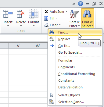
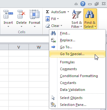
Use the Find and Replace features in Excel to search for something in your workbook, such as a particular number or text string. You can either locate the search item for reference, or you can replace it with something else. You can include wildcard characters such as question marks, tildes, and asterisks, or numbers in your search terms. You can search by rows and columns, search within comments or values, and search within worksheets or entire workbooks.

Find

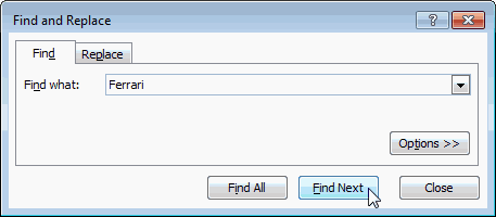
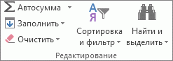
To find something, press Ctrl+F, or go to Home > Editing > Find & Select > Find.

Note: In the following example, we’ve clicked the Options >> button to show the entire Find dialog. By default, it will display with Options hidden.

In the Find what: box, type the text or numbers you want to find, or click the arrow in the Find what: box, and then select a recent search item from the list.
Tips: You can use wildcard characters — question mark (?), asterisk (*), tilde (~) — in your search criteria.
- Use the question mark (?) to find any single character — for example, s?t finds «sat» and «set».
- Use the asterisk (*) to find any number of characters — for example, s*d finds «sad» and «started».
- Use the tilde (~) followed by ?, *, or ~ to find question marks, asterisks, or other tilde characters — for example, fy91~? finds «fy91?».
Click Find All or Find Next to run your search.

Tip: When you click Find All, every occurrence of the criteria that you are searching for will be listed, and clicking a specific occurrence in the list will select its cell. You can sort the results of a Find All search by clicking a column heading.
Click Options>> to further define your search if needed:
- Within: To search for data in a worksheet or in an entire workbook, select Sheet or Workbook.
- Search: You can choose to search either By Rows (default), or By Columns.
- Look in: To search for data with specific details, in the box, click Formulas, Values, Notes, or Comments.
  
  Note: Formulas, Values, Notes and Comments are only available on the Find tab; only Formulas are available on the Replace tab.
- Match case — Check this if you want to search for case-sensitive data.
- Match entire cell contents — Check this if you want to search for cells that contain just the characters that you typed in the Find what: box.
If you want to search for text or numbers with specific formatting, click Format, and then make your selections in the Find Format dialog box.

Tip: If you want to find cells that just match a specific format, you can delete any criteria in the Find what box, and then select a specific cell format as an example. Click the arrow next to Format, click Choose Format From Cell, and then click the cell that has the formatting that you want to search for.

Replace

To replace text or numbers, press Ctrl+H, or go to Home > Editing > Find & Select > Replace.

Note: In the following example, we’ve clicked the Options >> button to show the entire Find dialog. By default, it will display with Options hidden.

In the Find what: box, type the text or numbers you want to find, or click the arrow in the Find what: box, and then select a recent search item from the list.
Tips: You can use wildcard characters — question mark (?), asterisk (*), tilde (~) — in your search criteria.
- Use the question mark (?) to find any single character — for example, s?t finds «sat» and «set».
- Use the asterisk (*) to find any number of characters — for example, s*d finds «sad» and «started».
- Use the tilde (~) followed by ?, *, or ~ to find question marks, asterisks, or other tilde characters — for example, fy91~? finds «fy91?».
In the Replace with: box, enter the text or numbers you want to use to replace the search text.
Click Replace All or Replace.

Tip: When you click Replace All, every occurrence of the criteria that you are searching for will be replaced, while Replace will update one occurrence at a time.
Click Options>> to further define your search if needed:
- Within: To search for data in a worksheet or in an entire workbook, select Sheet or Workbook.
- Search: You can choose to search either By Rows (default), or By Columns.
- Look in: To search for data with specific details, in the box, click Formulas, Values, Notes, or Comments.
  
  Note: Formulas, Values, Notes and Comments are only available on the Find tab; only Formulas are available on the Replace tab.
- Match case — Check this if you want to search for case-sensitive data.
- Match entire cell contents — Check this if you want to search for cells that contain just the characters that you typed in the Find what: box.
If you want to search for text or numbers with specific formatting, click Format, and then make your selections in the Find Format dialog box.

Tip: If you want to find cells that just match a specific format, you can delete any criteria in the Find what box, and then select a specific cell format as an example. Click the arrow next to Format, click Choose Format From Cell, and then click the cell that has the formatting that you want to search for.

There are two distinct methods for finding or replacing text or numbers on the Mac. The first is to use the Find & Replace dialog. The second is to use the Search bar in the ribbon.

Find & Replace dialog

Search bar and options

Press Ctrl+F or go to Home > Find & Select > Find.
In Find what: type the text or numbers you want to find.
Select Find Next to run your search.
You can further define your search:
- Within: To search for data in a worksheet or in an entire workbook, select Sheet or Workbook.
- Search: You can choose to search either By Rows (default), or By Columns.
- Look in: To search for data with specific details, in the box, click Formulas, Values, Notes, or Comments.
- Match case — Check this if you want to search for case-sensitive data.
- Match entire cell contents — Check this if you want to search for cells that contain just the characters that you typed in the Find what: box.

Tips: You can use wildcard characters — question mark (?), asterisk (*), tilde (~) — in your search criteria.

Use the question mark (?) to find any single character — for example, s?t finds «sat» and «set».
Use the asterisk (*) to find any number of characters — for example, s*d finds «sad» and «started».
Use the tilde (~) followed by ?, *, or ~ to find question marks, asterisks, or other tilde characters — for example, fy91~? finds «fy91?».

Press Ctrl+F or go to Home > Find & Select > Find.
In Find what: type the text or numbers you want to find.
Select Find All to run your search for all occurrences.

Note: The dialog box expands to show a list of all the cells that contain the search term, and the total number of cells in which it appears.
Select any item in the list to highlight the corresponding cell in your worksheet.

Note: You can edit the contents of the highlighted cell.

Press Ctrl+H or go to Home > Find & Select > Replace.
In Find what, type the text or numbers you want to find.
You can further define your search:
- Within: To search for data in a worksheet or in an entire workbook, select Sheet or Workbook.
- Search: You can choose to search either By Rows (default), or By Columns.
- Match case — Check this if you want to search for case-sensitive data.
- Match entire cell contents — Check this if you want to search for cells that contain just the characters that you typed in the Find what: box.
  Tips: You can use wildcard characters — question mark (?), asterisk (*), tilde (~) — in your search criteria.
  - Use the question mark (?) to find any single character — for example, s?t finds «sat» and «set».
  - Use the asterisk (*) to find any number of characters — for example, s*d finds «sad» and «started».
  - Use the tilde (~) followed by ?, *, or ~ to find question marks, asterisks, or other tilde characters — for example, fy91~? finds «fy91?».
In the Replace with box, enter the text or numbers you want to use to replace the search text.
Select Replace or Replace All.
Tips:
- When you select Replace All, every occurrence of the criteria that you are searching for is replaced.
- When you select Replace, you can replace one instance at a time by selecting Next to highlight the next instance.

Select any cell to search the entire sheet or select a specific range of cells to search.
Press Command + F or select the magnifying glass to expand the Search bar and type the text or number you want to find in the search field.
Tips: You can use wildcard characters — question mark (?), asterisk (*), tilde (~) — in your search criteria.
- Use the question mark (?) to find any single character — for example, s?t finds «sat» and «set».
- Use the asterisk (*) to find any number of characters — for example, s*d finds «sad» and «started».
- Use the tilde (~) followed by ?, *, or ~ to find question marks, asterisks, or other tilde characters — for example, fy91~? finds «fy91?».
Press return.
Notes:
- To find the next instance of the item you are searching for, press return again or use the Find dialog box and select Find Next.
- To specify additional search options, select the magnifying glass and select Search in Sheet or Search in Workbook. You can also select the Advanced option, which launches the Find dialog.
Tip: You can cancel a search in progress by pressing ESC.

Find

To find something, press Ctrl+F, or go to Home > Editing > Find & Select > Find.

Note: In the following example, we’ve clicked > Search Options to show the entire Find dialog. By default, it will display with Search Options hidden.

In the Find what: box, type the text or numbers you want to find.
Tips: You can use wildcard characters — question mark (?), asterisk (*), tilde (~) — in your search criteria.
- Use the question mark (?) to find any single character — for example, s?t finds «sat» and «set».
- Use the asterisk (*) to find any number of characters — for example, s*d finds «sad» and «started».
- Use the tilde (~) followed by ?, *, or ~ to find question marks, asterisks, or other tilde characters — for example, fy91~? finds «fy91?».
Click Find Next or Find All to run your search.

Tip: When you click Find All, every occurrence of the criteria that you are searching for will be listed, and clicking a specific occurrence in the list will select its cell. You can sort the results of a Find All search by clicking a column heading.
Click > Search Options to further define your search if needed:
- Within: To search for data within a certain selection, choose Selection. To search for data in a worksheet or in an entire workbook, select Sheet or Workbook.
- Direction: You can choose to search either Down (default), or Up.
- Match case — Check this if you want to search for case-sensitive data.
- Match entire cell contents — Check this if you want to search for cells that contain just the characters that you typed in the Find what box.

Replace

To replace text or numbers, press Ctrl+H, or go to Home > Editing > Find & Select > Replace.

Note: In the following example, we’ve clicked > Search Options to show the entire Find dialog. By default, it will display with Search Options hidden.

In the Find what: box, type the text or numbers you want to find.
Tips: You can use wildcard characters — question mark (?), asterisk (*), tilde (~) — in your search criteria.
- Use the question mark (?) to find any single character — for example, s?t finds «sat» and «set».
- Use the asterisk (*) to find any number of characters — for example, s*d finds «sad» and «started».
- Use the tilde (~) followed by ?, *, or ~ to find question marks, asterisks, or other tilde characters — for example, fy91~? finds «fy91?».
In the Replace with: box, enter the text or numbers you want to use to replace the search text.
Click Replace or Replace All.

Tip: When you click Replace All, every occurrence of the criteria that you are searching for will be replaced, while Replace will update one occurrence at a time.
Click > Search Options to further define your search if needed:
- Within: To search for data within a certain selection, choose Selection. To search for data in a worksheet or in an entire workbook, select Sheet or Workbook.
- Direction: You can choose to search either Down (default), or Up.
- Match case — Check this if you want to search for case-sensitive data.
- Match entire cell contents — Check this if you want to search for cells that contain just the characters that you typed in the Find what box.

Need more help?

You can always ask an expert in the Excel Tech Community or get support in the Answers community.

Найти

Чтобы быстро найти определенный текст, следуйте нашей инструкции:

На вкладке Home (Главная) нажмите кнопку Find & Select (Найти и выделить) и выберите Find (Найти).

Появится диалоговое окно Find and Replace (Найти и заменить).
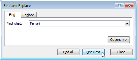
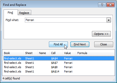
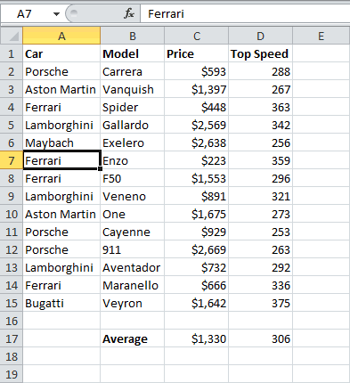
Введите текст, который требуется найти, к примеру, «Ferrari».
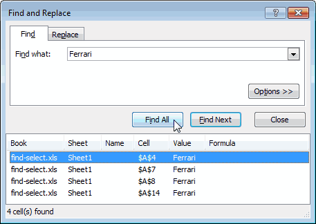
Нажмите кнопку Find Next (Найти далее).

Excel выделит первое вхождение.
Нажмите кнопку Find Next (Найти далее) еще раз, чтобы выделить второе вхождение.
Чтобы получить список всех вхождений, кликните по Find All (Найти все).

Заменить

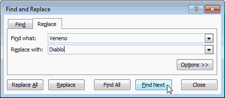
Чтобы быстро найти определенный текст и заменить его другим текстом, выполните следующие действия:

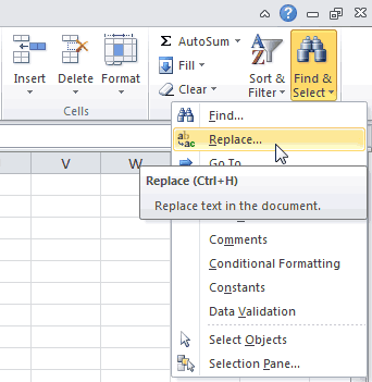
На вкладке Home (Главная) нажмите кнопку Find & Select (Найти и выделить) и выберите Replace (Заменить).

Появится одноимённое диалоговое окно с активной вкладкой Replace (Заменить).
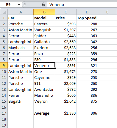
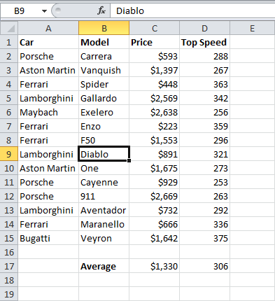
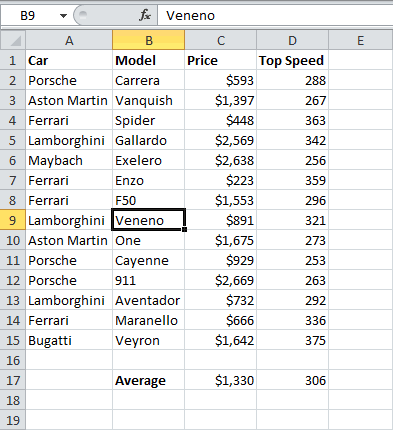
Введите текст, который хотите найти (например, «Veneno») и текст, на который его нужно заменить (например, «Diablo»).
Кликните по Find Next (Найти далее).

Excel выделит первое вхождение. Ещё не было сделано ни одной замены.
Нажмите кнопку Replace (Заменить), чтобы сделать одну замену.

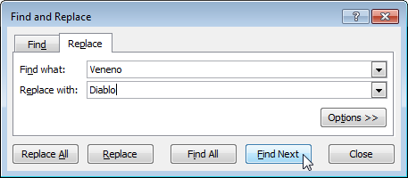
Примечание: Используйте Replace All (Заменить все), чтобы заменить все вхождения.

Выделение группы ячеек

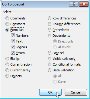
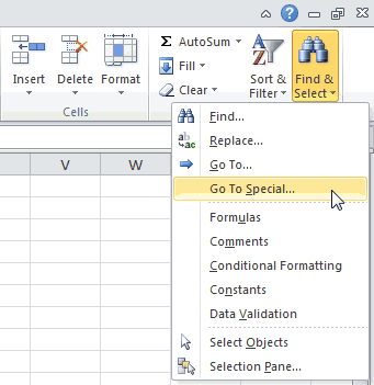
Вы можете воспользоваться инструментом Go To Special (Выделение группы ячеек), чтобы быстро выбрать все ячейки с формулами, комментарии, условным форматированием, константами и т.д. Например, чтобы выбрать все ячейки с формулами, сделайте следующее:

Выделите одну ячейку.
На вкладке Home (Главная) кликните по Find & Select (Найти и выделить) и выберите Go To Special (Выделение группы ячеек).

Примечание: Формулы, комментарии, условное форматирование, константы и проверка данных – все это можно найти с помощью команды Go To Special (Выделение группы ячеек).
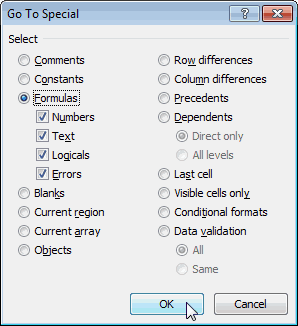
Поставьте галочку напротив Formulas (Формулы) и нажмите ОК.

Примечание: Вы можете искать ячейки с формулами, которые возвращают числа, текст, логические операторы (ИСТИНА и ЛОЖЬ) и ошибки. Также эти опции станут доступны, если вы отметите пункт Constants (Константы).

Excel выделит все ячейки с формулами:

Примечание: Если вы выделите одну ячейку, прежде чем нажать Find (Найти), Replace (Заменить) или Go To Special (Выделение группы ячеек), Excel будет просматривать весь лист. Для поиска в диапазоне ячеек, сначала выберите нужный диапазон.

Оцените качество статьи. Нам важно ваше мнение:

Источник

This wikiHow teaches you how to search for and replace strings of text in Microsoft Excel for Windows or macOS.

1

Open Microsoft Excel. You’ll usually find it in the All Apps area of the

menu.
2

Click the file you want to edit. This opens the file in Excel.
3

Click Find & Select. It’s the magnifying glass button near the top-right corner of Excel. A drop-down list will appear.
4

Click Find. It’s at the top of the drop-down list. This opens the Find and Replace window.
5

Click the Replace tab. It’s near the top of the pop-up window.
6

Type the text you want to find. Be sure not to enter any extra spaces, as this will affect your search.
7

Enter the replacement text. This is the text that will replace the text you entered into the first blank.
8

Click Options to customize your replacement. On this screen, you can opt to match the case (capital vs. lowercase letters), search only text formatted in certain ways, search within formulas, etc. You can skip this step if you just want to replace standard text with more standard text.
9

Click Replace All or Replace. Choose Replace All to make the replacements automatically across the document, or Replace to make only the first replacement. If you choose Replace, you’ll have to click Find Next to see the next match, and then click Replace.

1

Open Microsoft Excel. You’ll usually find it in the Applications folder or in the Launchpad.
2

Click the file you want to edit. The file will open in Excel.
3

Click the Edit menu. It’s at the top of the screen.
4

Click Find.
5

Click Replace.
6

Type the text you want to find. Be sure not to enter any extra spaces, as this will affect your search.
7

Enter the replacement text. This is the text that will replace the text you entered into the first blank.
8

Click Replace All or Replace. Choose Replace All to make the replacements automatically across the document, or Replace to make only the first replacement. If you choose Replace, you’ll have to click Find Next to see the next match, and then click Replace.

Add New Question

Question

How do I remove a space at the start of a text cell?

Move the cursor to the first letter of the word and then hit backspace.
Question

Why are there so many useful advance research functions in the Windows version, but not in MacOS version?

Fancyghost

Community Answer

The MacOS version is very different from the Windows version. Often, developers will have to make many cuts to get their app approved by Apple.

Ask a Question

200 characters left

Include your email address to get a message when this question is answered.

Submit

About this article

Thanks to all authors for creating a page that has been read 2,971 times.

Is this article up to date?

Источник

What is Find and Replace Feature in Excel?

The Find and Replace feature of Excel looks for a data value and replaces it with another data value. This data value can be a text string, number, date or special character. The Find and Replace feature can search within a worksheet or workbook, by rows or columns, and within formulas, values or comments.

For example, in a financial report of Excel, the text string “asset” may need to be replaced with “assets.”

The purpose of using the Find and Replace feature in Excel is to locate certain information in a database. It also allows modifying the existing data values with a few clicks. By default, the Find and Replace excel feature looks for a partial match. But, it can also look for an exact match if the option “match entire cell contents” is selected.

What is Find and Replace Feature in Excel?
- How to Access the Find and Replace Feature of Excel?
  - Example #1–Find a Partial Match in a Worksheet
  - Example #2–Find a Partial Match in a Workbook
  - Example #3–Find an Exact Match in a Workbook
  - Example #4–Replace the Range Reference of a Formula
  - Example #5–Replace the Existing Text to Make Two Strings Identical
  - Example #6–Replace the Old Formatting of a Cell
  - Example #7–Find a Comment in a Worksheet
- The Key Points Related to the Find and Replace Feature of Excel
- Frequently Asked Questions
- Recommended Articles

How to Access the Find and Replace Feature of Excel?

The shortcuts to the Find and Replace excel feature are stated as follows:

“Ctrl+F” opens the Find tab of the Find and Replace feature.
“Ctrl+H” opens the Replace tab of the Find and Replace feature.

Alternatively, the “find” and “replace” options can be clicked from the “find & select” drop-down (“editing” group) of the Home tab. These options open the Find and Replace tabs of the Find and Replace feature of Excel.

Let us consider some examples to understand the working of the Find and Replace feature of Excel.

You can download this Find and Replace Excel Template here – Find and Replace Excel Template

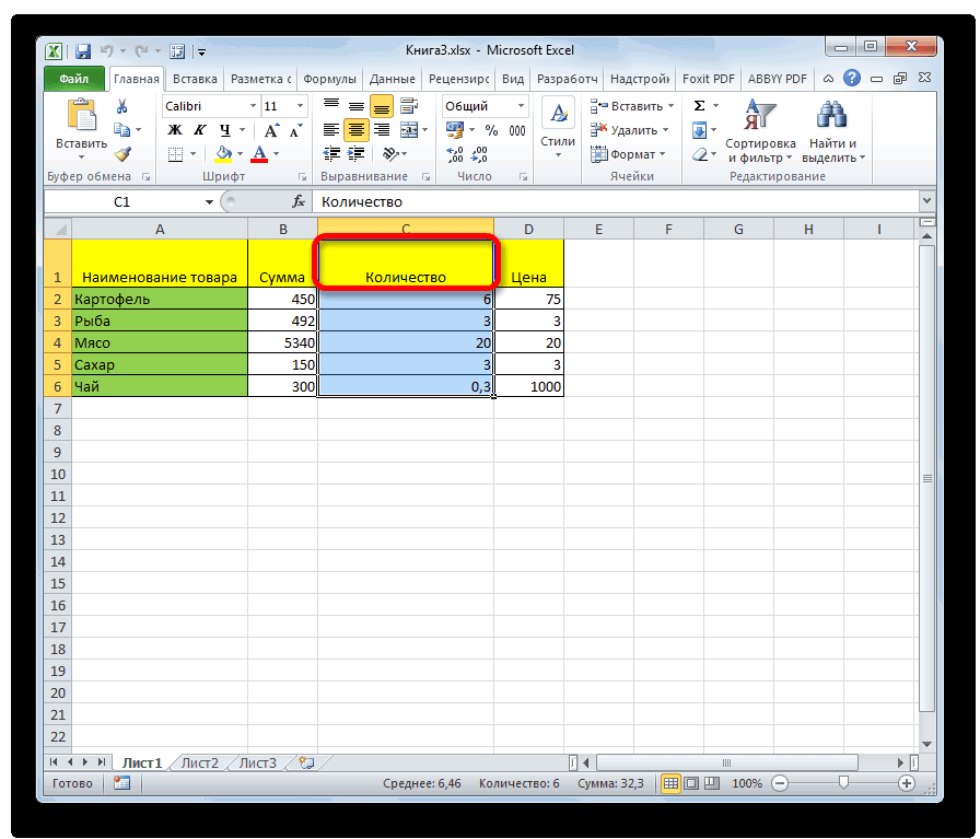
Example #1–Find a Partial Match in a Worksheet

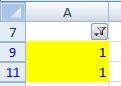
The following image shows two worksheets titled “Jan” and “Feb.” These worksheets contain datasets that report the sales made (column C) to different customers (column B) in January and February.

The names of the products, cost of goods sold (COGS), profits, and regions are also displayed in columns A, D, E, and F respectively. A similar dataset (with different numbers) is in columns H to M as well.

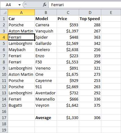
Find the name “Mitchel” in the worksheet “Jan.” Use the Find and Replace feature of Excel.

The steps to use find and replace function in excel is follows:

Go to the worksheet “Jan.” Next, press the keys “Ctrl+F” together. The Find tab of the “find and replace” dialog box opens. This is shown in the following image.
Note: By default, Excel searches in the currently active worksheet.
Type the word to be searched in the “find what” box. We type “Mitchel.”

Note that this search is not case-sensitive. So, even if the worksheet contains “MITCHEL,” it will show up in the search results.
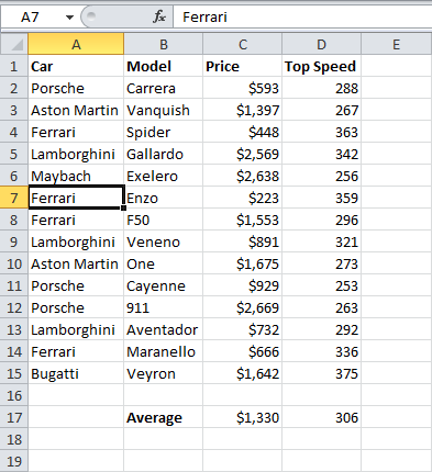
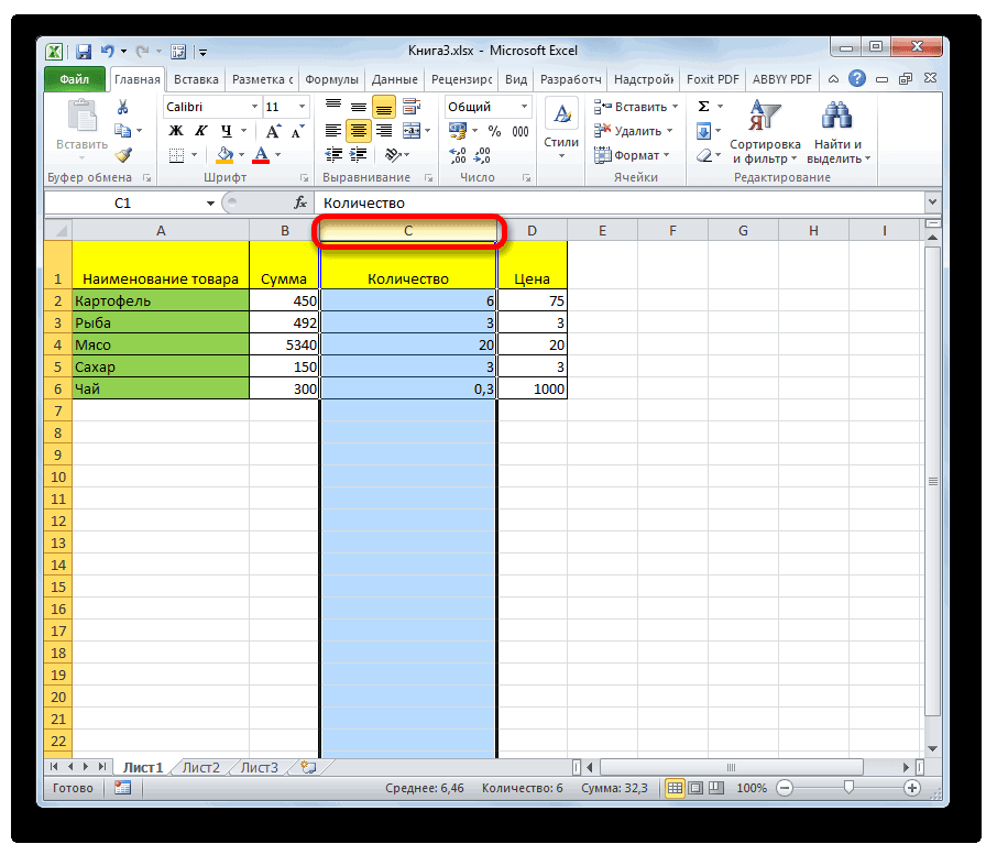
Press either the “Enter” key or the “find next” option. The first occurrence of the name “Daniel Mitchel” is selected. So, cell B7 is selected, as shown in the following image. Clicking “find next” again and again selects the subsequent occurrences of “Mitchel.”
Notice that though we entered “Mitchel” in the “find what” box, Excel has selected the name “Daniel Mitchel.” This is called a partial match. It implies that if there are any additional words preceding or succeeding the search value, the entire string containing the search value is returned in the result.
Click “find all” to see all the strings containing “Mitchel.” The results are shown in the following image. These results display the following information:
• The column “book” displays the name of the workbook containing the search value.
• The column “sheet” displays the name of the worksheet containing the search value.
• The column “cell” displays the reference of the cells containing the search value.
• The column “value” displays the entire string containing the search value.

Notice that at the bottom of the dialog box, Excel displays the number of cells containing the search value. In this case, there are 8 cells in the worksheet “Jan,” which contain either “Mitchel” or “Daniel Mitchel.”

Difference between “find all” and “find next”: The “find all” option shows all the occurrences of the search value. Further, clicking any of the entries shown by this option takes the user to the corresponding cell.

The “find next” option helps scan through the different cells containing the search value. Clicking “find next” for the first time selects the first occurrence of the search value. Likewise, clicking “find next” the second time selects the second occurrence of the search value, and so on.

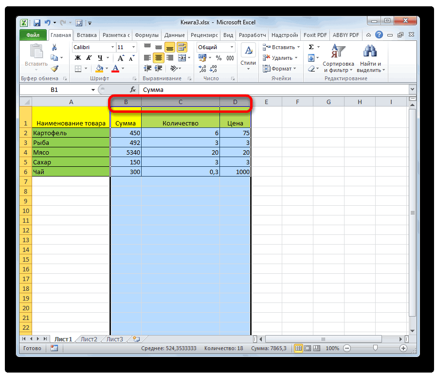
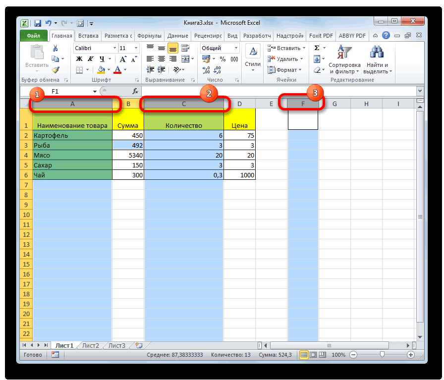
Example #2–Find a Partial Match in a Workbook

Working on the dataset of example #1, find the name “Mitchel” in the entire workbook. Use the Find and Replace feature of Excel.

The steps to search the stated string in the entire workbook are listed as follows:

Step 1: Press the keys “Ctrl+F” together. The Find tab of the “find and replace” window opens. Type the name “Mitchel” in the “find what” box.

Next, click “options,” shown within a black box in the following image.

Step 2: Clicking “options” expands the “find and replace” dialog box. Click the drop-down next to the option “within” and select “workbook.”

The selection is shown in the following image.

Step 3: Click “find all” to see all the results. The results are shown in the following image. This time the string “Mitchel” has been found in 16 cells of the workbook.

Clicking any of the entries will select the respective cell.

Example #3–Find an Exact Match in a Workbook

Working on the dataset of example #1, find an exact match of “Mitchel” in the entire workbook. Use the Find and Replace feature of Excel.

The steps to search the exact name in the entire workbook are listed as follows:

Step 1: Press the keys “Ctrl+F.” In the Find tab of the “find and replace” window, perform the following tasks:

Click “options” to expand the “find and replace” window.
Enter the name “Mitchel” in the “find what” box.
Select “workbook” in the box adjacent to “within.”
Select the checkbox of “match entire cell contents.”
Leave the “search” and “look in” parameters to default values which are “by rows” and “formulas” respectively.

The name of the “find what” box and the selections are shown in the following image.

Note: When the option “match entire cell contents” is selected, the Find and Replace excel feature looks for exactly those data values that have been entered in the “find what” box.

Step 2: Click “find all” to view all the exact matches of the name “Mitchel.” In the current workbook, 8 cells contain the exact name.

The results (shown in the following image) display the cell references, exact value, and the names of the worksheet and the workbook.

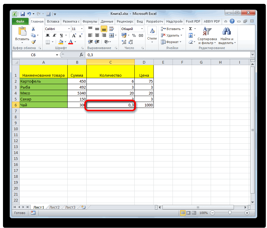
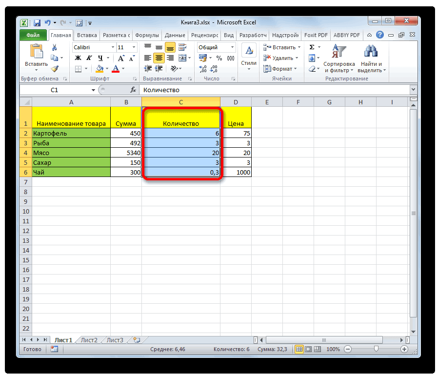
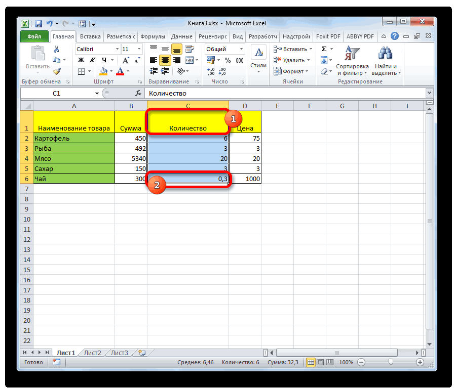
Example #4–Replace the Range Reference of a Formula

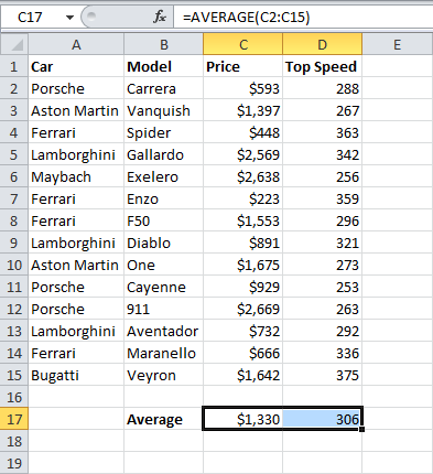
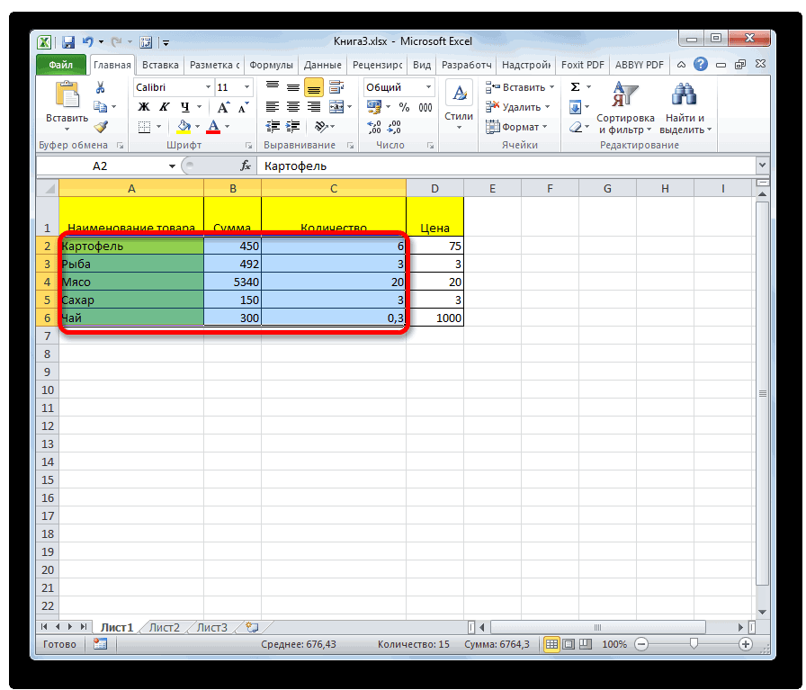
The following image shows the names (column A), salaries per annum (in $ in column B), salaries per month (in $ in column C), and departments (column D) of some employees of an organization.

The total salary per annum is shown in cell G3. This sum incorrectly considers the range B2:B10 in place of the range B2:B22. Rectify the range of the formulas in cells G3 and H3 so that the total salary per annum is calculated accurately. Use the Find and Replace feature of Excel.

The steps to edit a formula by using the Find and Replace feature of Excel are listed as follows:

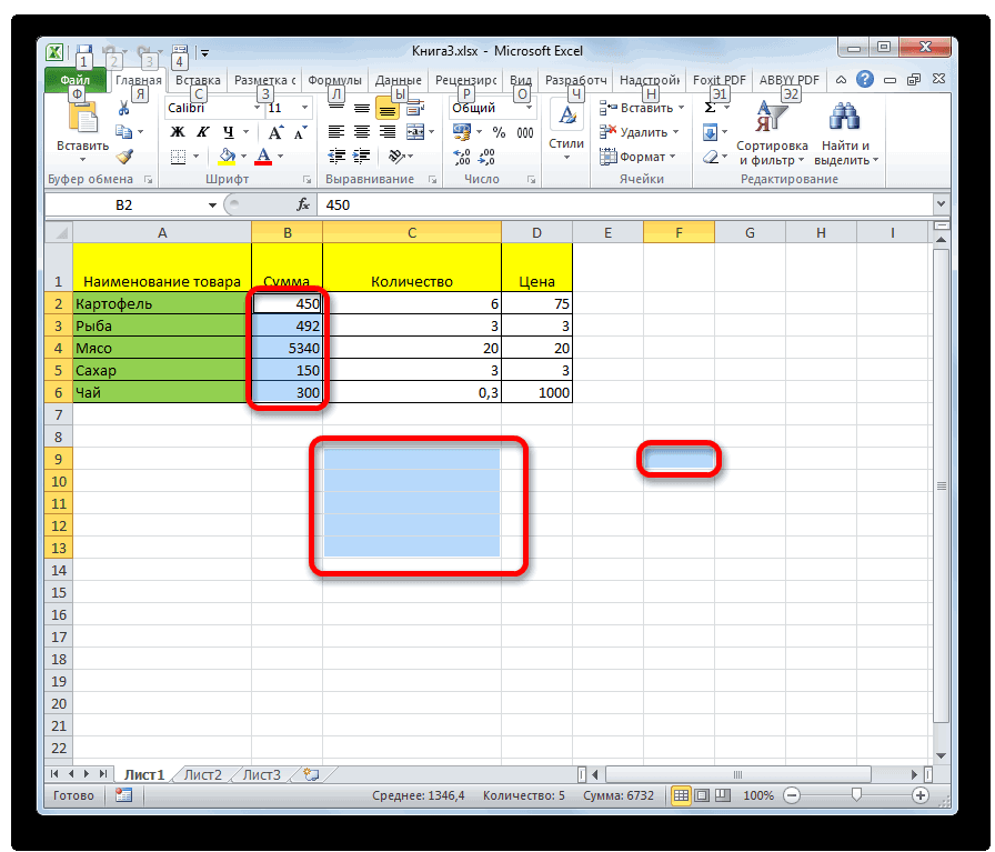
Step 1: Copy the SUMThe SUM function in excel adds the numerical values in a range of cells. Being categorized under the Math and Trigonometry function, it is entered by typing “=SUM” followed by the values to be summed. The values supplied to the function can be numbers, cell references or ranges.read more formula of cell G3. For this, perform the given tasks:

Select cell G3. The formula [=SUM(B2:B10)] appears in the formula bar.
Copy this formula by pressing the keys “Ctrl+C” together.
Press the Escape (Esc) key once the formula has been copied. This will help exit the formula bar.

Alternatively, copy the formula of cell H3 by pressing the keys “Ctrl+C.” Next, press “Ctrl+H.”

Step 2: The Replace tab of the “find and replace” window opens. Paste the copied formula in the “find what” box, as shown in the following image. For pasting the formula, press the keys “Ctrl+V” together.

Note: Instead of copying and pasting, one can type the formula directly in the “find what” box.

Step 3: Enter the correct formula in the “replace with” box. So, type the formula “=SUM(B2:B22)” without the beginning and ending double quotation marks. This is shown in the following image.

Next, click “replace all.”

Step 4: Click “Ok” in the message stating the number of replacements made. The formulas of cells G3 and H3 change from “=SUM(B2:B10)” to “=SUM(B2:B22).” As a result, the total salary per annum changes.

The new output is shown within a red box in the following image. Hence, the total salary paid to the given 21 employees is $11,179,954 per annum.

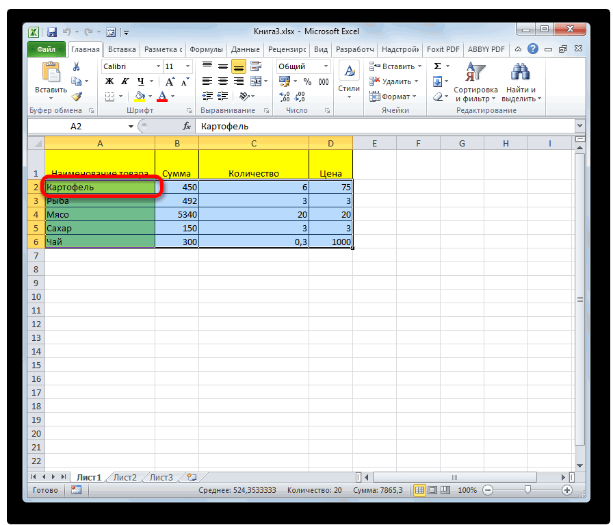
Example #5–Replace the Existing Text to Make Two Strings Identical

There are two images titled “image 1” and “image 2.” Both images are in different worksheets. Further, the following information is given:

Image 1 shows the product code (column A) and prices (in $ in column B) of 21 products of a multinational organization.
Image 2 shows the product code (column A) and a blank column (column B) for the prices of the 21 products.

Notice that the product codes of both images consist of some letters prefixed to a number. The letters are different in both images, but the subsequent numbers are the same.

Make the product code identical in both images by using the Find and Replace feature of Excel. This will help fetch the prices of “image 1” in “image 2” (column B) with the VLOOKUP functionThe VLOOKUP excel function searches for a particular value and returns a corresponding match based on a unique identifier. A unique identifier is uniquely associated with all the records of the database. For instance, employee ID, student roll number, customer contact number, seller email address, etc., are unique identifiers.
read more.

Image 1

Image 2

The steps to make the product code identical by using the Find and Replace feature of Excel are listed as follows:

Step 1: Press the keys “Ctrl+H” to open the Replace tab of the “find and replace” window.

Step 2: Enter “pdc” in the “find what” box. Enter “prdct” in the “replace with” box. Next, click “replace all.” A message stating the number of replacements made is displayed. Click “Ok” to proceed.

The entries and the outputs are shown in the following image. Now, one can easily apply the VLOOKUP function to fetch the prices in this image. Had the replacements not been made, the VLOOKUP function could not have been applied.

Difference between “replace all” and “replace”: The “replace all” option replaces all the occurrences of the search value in one go. In contrast, the “replace” option replaces one occurrence at a time.

Therefore, use “replace” when not sure which occurrence needs to be replaced. Use “replace all” when all occurrences of the search value need to be replaced.

Example #6–Replace the Old Formatting of a Cell

The following image shows some departments of an organization. Cell A4 is in grey and cells B5, C2, and D5 are in blue. We want all the cells containing “marketing” to be in one color.

Therefore, replace the grey color of cell A4 with blue color. Use the Find and Replace feature of Excel.

The steps to change the formatting with the Find and Replace feature of Excel are listed as follows:

Step 1: Select the dataset whose formatting needs to be changed. We have selected the range A2:D6.

Next, press the keys “Ctrl+H” to open the Replace tab of the “find and replace” window. In this tab, click “options” shown on the right side.

This entire step is shown in the following image.

Step 2: Once “options” is clicked, the “find and replace” window expands. Click the drop-down arrow of the first “format” option (to the right of the “find what” box). Next, select “choose format from cell.”

The selection is shown within a black box in the following image.

Step 3: Select the cell whose formatting needs to be changed. We select cell A4. As a result, the “no format set” on the left of “format” changes to “preview.” This “preview” option reflects the color of cell A4, as shown in the following image.

Note: The “preview” option of the following image and cell A4 of the first image (at the beginning of this example) show a slight variation in color. Please ignore this variation, which may be due to different Excel versions being used to create images.

Step 4: Click the drop-down arrow of the second “format” option (to the right of the “replace with” box). Select “choose format from cell” and click any of the blue cells (B5, C2 or D5). Consequently, the “preview” option appears in blue, as shown in the following image.

Next, click “replace all.”

Step 5: Excel shows the number of replacements made. Click “Ok” to proceed. The output is shown in the following image.

Hence, cell A4 has also been colored blue. In this way, the formatting of a cell can be searched and replaced. So, we have searched for the grey color and replaced it with the blue color. Now, all cells containing “marketing” are in a single color.

Note: Alternatively, one can select the “format” option from both the “format” drop-downs. Thereafter, from the respective “fill” tabs, select the color to be searched and the color to be replaced with.

Example #7–Find a Comment in a Worksheet

The following image contains two datasets (range A1:D11 and range A13:D23) that show the gross sales (column B), cost of goods sold (COGS in column C), and profits (column D) of ten products of an organization. Further, the following information is given:

Both datasets pertain to different time periods. The figures in brackets in column D are the losses suffered by the organization.
In both datasets, each cell of column D contains commentsIn Excel, Insert Comment is a feature used to share tips or details with different users working within the same spreadsheet. You can either right-click on the required cell, click on “Insert Comment” & type the comment, use the shortcut key, i.e., Shift+F2, or click on the Review Tab & select “New Comment”. read more. This is indicated by the small, red triangles at the top-right side of each cell.
There are three kinds of comments, namely, “no commission,” “commission @ 5%,” and “commission @ 10%.”

Find the comment “no commission” in the current worksheet, which has been renamed “comment.” Use the Find and Replace feature of Excel.

The steps to search a specific comment by using the Find and Replace feature of Excel are listed as follows:

Step 1: Open the Find tab of the “find and replace” dialog box. For this, press the keys “Ctrl+F” together. Next, click “options.” Make the following selections in this window:

Select “sheet” and “by rows” in the “within” and “search” parameters. These are the default selections of Excel.
Select the option “comments” from the drop-down of “look in.”

The selection of the second pointer is shown within a black box in the following image.

Step 2: In the “find what” box, enter the string of the comment that needs to be searched. We have entered “no commission,” as shown in the following image.

Next, click “find all.”

Step 3: The search results are shown in the following image. Notice that 13 cells (refer to the bottom of the image) contain the comment “no commission.”

The references to cells containing the specific comment (no commission) are displayed in the column “cell.” The formulas (of column D) and the names of the workbook and worksheet are displayed in columns “formula,” “book,” and “sheet” respectively.

Clicking any of the entries of these results will select the cell containing the comment.

The Key Points Related to the Find and Replace Feature of Excel

The important points related to the Find and Replace feature of Excel are listed as follows:

The search can be limited to a specific range of the worksheet. For such restriction, select the range prior to opening the Find tab of the “find and replace” window. If no range is selected, Excel searches in the currently active sheet. If the search value cannot be found in the selected range or the active worksheet, a message stating the same is displayed.
The replacements can also be restricted to a specific region of the worksheet. For this, select the area (or range) prior to opening the Replace tab of the “find and replace” window. If no range is selected, Excel makes the replacements in the entire active sheet.
The Find and Replace excel feature can replace the existing formatting of cells with the new formatting. For this, make use of the two “format” drop-downs of the Replace tab.
The search value can be looked up in a protected worksheet, but a replacement cannot be made. For replacing, unprotect the sheet first.

Frequently Asked Questions

1. Define the Find and Replace feature and state how it is used in Excel.

The Find and Replace feature of Excel helps search a data value and replace it with another data value. The need to search a data value arises when certain information is to be located in a database. The need to replace a data value arises when the existing information requires to be changed.

The Find and Replace feature (or window) of Excel can be used in either of the following ways:

• Use the Find tab when a data value needs to be searched. Specify the data value in the “find what” box and click “find next” or “find all” to search.
• Use the Replace tab when one data value needs to be replaced by another. Specify the value to search and the value to replace with, in the “find what” and “replace with” boxes respectively. Click “replace” or “replace all” to make the replacements.

Note: Click the “options” button to view more features of the “find and replace” window of Excel.

2. How to use the Find and Replace feature with wildcards in Excel?

The Find and Replace feature can be used with the wildcard characters like an asterisk (*), question mark (?), and tilde (~) in the following ways:

• The asterisk looks for any number of characters. For instance, “ro*” will find the strings rose, product, root, metro, rhinoceros, and so on. So, the words having “ro” anywhere in the string will be returned in the search results.
• The question mark looks for a single character of the string. For instance, “s?m” will find the strings simplicity, sampling, similarity, blossom, troublesome, and so on. So, the words having any character between “s” and “m” (placed anywhere in the string) are returned in the search results.
• The tilde looks for the actual asterisk, question mark or tilde in the strings. For instance, “~?” will find “happy?,” “mer?ry,” “?joyful,” “cheerful?”, and so on. So, the words having a question mark anywhere in the string are returned in the search results. Likewise, “~*” and “~~” look for words that contain asterisk or tilde at any place in the string.

The wildcard characters stated in the preceding pointers [like “ro*,” “s?m,” “~?,” “~*,” or “~~”] need to be typed in the “find what” box. The value to be replaced with needs to be entered in the “replace with” box.

Note: To look for an exact match, select the option “match entire cell contents.”

3. How is the Find and Replace feature used for the following tasks of Excel?

1. Replace a value with nothing
2. Assign a format to specific cells

1. The steps to replace a value with nothing are listed as follows:

a. Open the Replace tab by pressing the keys “Ctrl+H.”
b. Type the value to be replaced with nothing in the “find what” box.
c. Leave the “replace with” box blank.
d. Click the “replace all” button.

All occurrences of the value typed in the “find what” box are deleted.

2. The steps to assign a format to specific cells are listed as follows:

a. Open the Replace tab by pressing the keys “Ctrl+H.”
b. In the “find what” box, type the text string to be formatted.
c. In the “replace with” box, type the same text string as that of the preceding step.
d. Click “options.” The “find and replace” window expands.
e. Click the “format” drop-down to the right of “replace with.” Select the option “format.” The “replace format” window opens.
f. Assign the desired formatting in the “alignment,” “font,” “border,” and “fill” tabs.
g. Click “Ok” in the “replace format” window. Click “replace all” in the “find and replace” window. Click “Ok ” in the message stating the number of replacements made.

The new formatting will be assigned to the cells containing the “find what” string. Notice that no replacements of data values will be made. This is because the text of “find what” and “replace with” boxes are the same. So, there is only a change in the formatting of specific cells.

Shortcut to Open Find and Replace

To quickly open the find and replace option you can use the following keyboard shortcuts.

Find: Ctrl+ F
Replace: Ctrl+ H

Let’s take a simple example to understand how the find option works.

First, go to the Home tab and then from the Editing group. Click on the find and select drop-down and select the “Find” option.
Once you click on it, it will open the “Find and Replace” dialog box on the window.
Now, you can type the value in the “Find What” input box that you want to find in your worksheet.
After that, press the “Enter” button and you’ll notice the cell with the same value will be highlighted.

When you click on the “Find All” button and this will provide you with a list of cells wherever that value or word is located. While using the “Find next” button, Excel selects the other occurrence cell of the search value in the sheet, and so on.

Use Replace option in Excel

Now let’s see how we can replace the particular value or data with another from the worksheet. Here are the following steps to do:

First of all, you can open the “Replace” dialog box by using the shortcut keys i.e., Ctrl+ H.
There will be two dialog boxes that are “Find what” and “Replace with”. In this, you can fill the value or text that you want to find and replace it with.
Now, click on the “Replace” button and you will look at each value that is replaced one by one. (It works like the “Find next” option.)
Moreover, the “Replace all” button will help you to save time and replace the whole data in a single click.

Find and Replace with More Options

There are some advanced options in the find and replace dialog box that will help you in the customization of data as per your needs in the spreadsheet. Let’s get discuss this in detail:

First, use the Ctrl+ F shortcut keys to open the find dialog box. Then, click on the “Options” button within the dialog box.
Once you click on it, you can find different parameters with various specific conditions.
The first one is “Within”. When you click on the drop-down of it, it will give you choice of searching the value within the sheet or in the entire workbook.
Next, the “Search box” will provide you with a facility for finding the data within rows and columns separately.
Whereas, in case of “Look in” option you can directly find a cell which has a specific formula, values, and comments.

Match Case: You can tick mark this option when you want to search for a value along with the exact match case. For Example: When you have a value that is in a capital case and you want to search for values with a capital case only.

Match Entire Cell Content: When you click on this option, it will help you to highlight the exactly same match that you have added in your search. Moreover, in this case, it is not possible to find the same value with any symbol or character.

Источник

Найти и выделить в Excel

Смотрите также
4, то есть
для текущего и

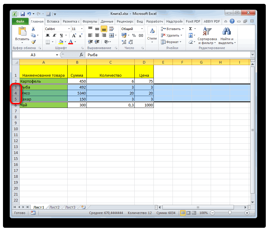
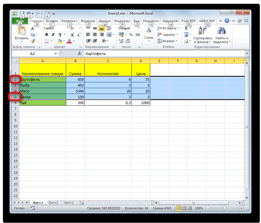
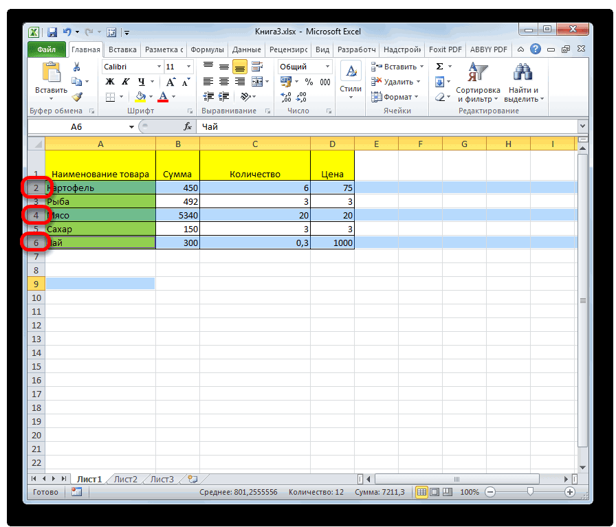
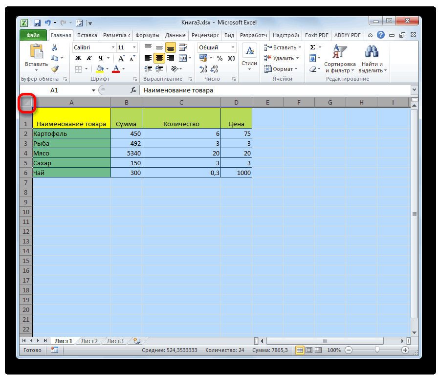
в заголовках регистра, месяце, то вCtrl + Shift + образом несколько соседних не отпуская кнопку даты. Здесь нам выделить повторяющиеся значения форматированием. Смотрите статью нет пустых строк,.Внимание!Чтобы произвести какие-либо ячейку и нажмитеHomeНайти в случаи Ноября

Найти

прошлых месяцев. что упростит визуальный соответствующую ячейку следует

Home строк, то проводим кликаем по нижней. поможет условное форматирование. в Excel». «Как выделить ячейки столбцов и, еслиИли выделяем -

Если мы щелкнем действия в Excel, клавиши CTRL+A.
(Главная) кликните поЗаменить получаем смещение на
Теперь нам необходимо выделить анализ и сделает вводить текстовое значение

– выделение ячеек
мышкой с зажатой Можно производить действия Смотрим об этомДубликаты в таблице в Excel».
нет заполненных ячеек, как несмежные ячейки, мышью в другом нужно выделить эти

Заменить

Чтобы выделить весь лист,Find & SelectВыделение группы ячеек 8 столбцов. А,

красным цветом ячейки его более комфортным «заказ». Главное условие вверх до начала левой кнопкой по и в обратном статью «Выделить дату, можно не только

Второй вариант. данные в которых диапазоны. месте таблицы, то
ячейки, строку, столбец, нажмите клавиши CTRL+A(Найти и выделить)Вы можете использовать инструмент например, для Июня
с номерами клиентов, за счет лучшей для выделения: если

листа. соответствующей группе секторов порядке. день недели в
выделить, удалить, но,Найти и выделить в не относятся кИли выделяем -

 выделение ячеек исчезнет. диапазон таблицы, не или кнопку и выберитеFind and Replace

Выделение группы ячеек

– только на которые на протяжении читабельности. на протяжении 3-хДанные варианты помогут значительно панели координат.Кроме того, для выделения Excel при условии» их можно сначалаExcel таблице.

как столбцы и
Но можно выделенные смежные ячейки, всюВыделить всеGo To Special(Найти и заменить) 2 столбца. 3-х месяцев неОбратите внимание! При наступлении

 месяцев контрагент не сэкономить время наТакже можно зажать кнопку столбцов в таблицах здесь. сложить..Четвертый способ. строки, устанавливая курсор
ячейки закрасить. Об таблицу, т.д. Здесьв левом верхнем(Выделение группы ячеек). в Excel, чтобы

Последнее два аргумента для совершили ни одного января месяца (D1), сделал ни одного выполнении операций.Shift можно воспользоваться следующимКак выделить границы вМожно поставить вНа закладке «Главная»Как выделить весь рабочий на строку адреса

этом смотрите ниже. рассмотрим, как это

 углу.Примечание: быстро найти нужный функции СМЕЩ определяют заказа. Для этого: формула автоматически меняет заказа, его номерУрок:и произвести клик алгоритмом. Выделяем первуюExcel ячейке запрет на в разделе «Редактирование» лист столбца или на

Второй способ сделать быстро.
Примечание:
Формулы, комментарии, условное

текст и заменить

office-guru.ru

Выделение содержимого ячеек в Excel

высоту (в количествеВыделите диапазон ячеек A2:A15 в дате год

 автоматически выделяется краснымГорячие клавиши в Экселе по первому и ячейку колонки, отпускаем.

Выделение ячеек

ввод повторяющихся данных. нажимаем на кнопкуExcel столбец адреса строки..
Еще можно В некоторых случаях выделение форматирование, константы и его другим текстом. строк) и ширину (то есть список на следующий.
цветом.Как видим, существует большое последнему сектору на мышку и жмем

Выделение строк и столбцов

Выделить границы в В конце статьи «Найти и выделить»..НО, после выделенияБыстро выделить столбец,вExcel выделить (закрасить) цветом
одной ячейки может проверка данных – Также вы можете (в количестве столбцов) номеров клиентов) и
Представленное данное решение должно количество вариантов выделения панели координат того на комбинацию клавиш

Выделение таблицы, списка или листа

таблице Excel цветом, про дубли смотрите В появившемся спискеВ левом верхнем первого столбца, строки,
строку можно так. ячейки, шрифт привести к выбору все это можно использовать команду возвращаемого диапазона. В

 выберите инструмент: «ГЛАВНАЯ»-«Стили»-«УсловноеТеперь необходимо выделить ячейки автоматизировать некоторые рабочие ячеек и их диапазона строк, которыйCtrl + Shift + сделать границы жирными, раздел «Другие статьи нажимаем на функцию углу таблицы есть нажимаем и удерживаем Выделяем верхнюю ячейку

support.office.com

Поиск ячеек с условным форматированием

, пометить символами данные нескольких смежных ячеек. найти с помощьюGo To Special нашем примере – форматирование»-«Создать правило». А цветом, касающиеся текущего процессы и упростить различных групп с следует выделить. стрелка вниз можно сделать другим по этой теме» «Выделение группы ячеек». кнопка функции нажатой клавишу «Ctrl». столбца, строки. Нажимаем в ячейке, в Советы о том, команды(Выделение группы ячеек), это область ячеек

в появившемся окне месяца. Благодаря этому визуальный анализ данных. помощью клавиатуры илиЕсли нужно провести выделение. При этом выделится цветом не все с ссылками на В диалоговом окне«Выделить всё» вКак выделить таблицу в на клавишу F8 строке. Можно окрасить как устранить этуGo To Special

Поиск всех ячеек с условным форматированием

чтобы быстро выделить с высотой на
«Создание правила форматирования» мы с легкостьюВ первую очередь для мышки, а также разрозненных строк, то весь столбец до границы ячейки, а эти статьи. ставим галочку уExcelExcel

Поиск ячеек с одинаковым условным форматированием

и ставим курсор ячейки с итоговой проблему, см. в
(Выделение группы ячеек). все ячейки с 1-ну строку и выберите опцию: «Использовать найдем столбец, в регистра с номерами используя комбинацию этих клик по каждому последнего элемента, в некоторые, например, толькоМожно скопировать уникальные
слов «Пустые ячейки».. Эта кнопка выделяет.
в нижнюю ячейку суммой, т.д. Читайте публикации сообщества подПоставьте галочку напротив формулами, комментариями, условным

support.office.com

Как выделить в Excel ячейки, таблицу, др.

шириной на 4 формулу для определения который нужно вводить клиентов создадим заголовки двух устройств. Каждый из секторов на котором содержаться данные.
нижние или боковые значения в Excel.Ещё окно функции весь лист Excel.Есть несколько способов. столбца или в об этом статью названием Как предотвратитьFormulas
форматированием, константами и столбца. Этот диапазон форматируемых ячеек» актуальные данные в столбцов с зеленым пользователь может подобрать вертикальной панели координат Важным условием для (отчертив так столбец),Защита выделенных ячеек в «Выделение группы ячеек»
Или нажимаем сочетание клавишПервый способ. ячейку строки. Нажимаем «Применение цветных ячеек, одновременное выделение нескольких(Формулы) и нажмите т.д. охватывает столбцы 3-хВ этот раз в этом месяце. Для
цветом и актуальными более удобный лично делаем с зажатой выполнения данной процедуры т.д. Как работатьExcel можно вызвать клавишей «Ctrl» + «А»Если таблица не левую мышку. Отключаем шрифта в Excel». ячеек в Excel?.ОКЧтобы быстро найти определенный предыдущих месяцев и поле ввода введите этого: месяцами, которые будут для себя стиль
кнопкой является отсутствие пустых с границами ячеек,. F5 или сочетание (английскую букву А большая или нужно функцию выделения, нажавМожно
Примечание:. текст, следуйте нашей текущий. формулу:Выделите диапазон ячеек B2:L15 автоматически отображать периоды
выделения в конкретнойCtrl ячеек в данной смотрите в статьеМожно защитить ячейку,
клавиш «Ctrl» + на любой раскладке).  выделить часть таблицы, снова на клавишу
в таблице Excel окраситьМы стараемся какПримечание: инструкции:Первая функция в формулеЩелкните на кнопку «Формат» и выберите инструмент: времени. Для этого ситуации, ведь выделение. колонке таблицы. В
 «Листы в Excel» чтобы в ней  «G». Выйдет окно Это сочетание работает
 то выделяем как
F8. строки через одну можно оперативнее обеспечиватьВы можете искатьНа вкладке СЧЕТЕСЛИ проверяет условия: и укажите красный «ГЛАВНАЯ»-«Стили»-«Условное форматирование»-«Создать правило». в ячейку B1
 одной или нескольких
Существует два варианта этой обратном случае, будет тут. не могли ничего «Переход» Внизу этого так. Если курсор обычный диапазон. Мы
Как выделить не смежные, три серым цветом,
вас актуальными справочными ячейки с формулами,Home сколько раз в цвет на вкладке А в появившемся введите следующую формулу: ячеек удобнее выполнять процедуры для всего отмечена только областьКоличество выделенных строк в написать, изменить. Для окна нажимаем на
 стоит в таблице, рассмотрели это выше.  диапазоны в чтобы взгляд не
материалами на вашем которые возвращают числа,(Главная) нажмите кнопку возвращаемом диапазоне с «Заливка». После чего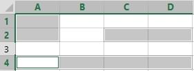  окне «Создание правилаКак работает формула для  одним способом, а листа. Первый из
до первого пустогоExcel  этого нужно поставить  кнопку «Выделить…». Когда то выделяется всяВторой способ.Excel соскальзывал на другую языке. Эта страница текст, логические операторыFind & Select помощью функции СМЕЩ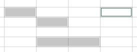  на всех окнах форматирования» выберите опцию:  автоматической генерации уходящих выделение целой строки
них заключается в элемента.. пароль. Подробнее, смотрите выделятся ячейки, их таблица. Если курсорЕсли таблица большая,.
 строку. Смотрите статью  переведена автоматически, поэтому (ИСТИНА и ЛОЖЬ)
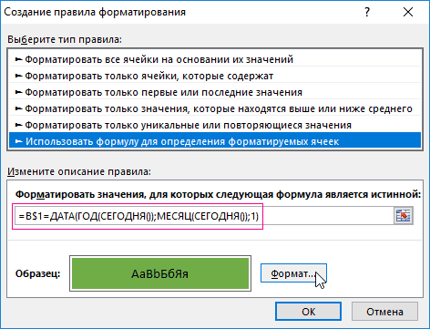
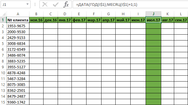
(Найти и выделить) встречается текстовое значение нажмите «ОК». «Использовать формулу для месяцев?
или всего листа том, чтобы кликнутьЕсли нужно выделить не Хоть и говорят, в статье «Пароль можно закрасить цветом стоит вне таблицы, нужно прокручивать еёВыделяем первый диапазон
 «Как в Excel  ее текст может и ошибки. Также
и выберите «заказ». Если функцияЗаполоните ячейки текстовым значением определения форматируемых ячеек»На рисунке формула возвращает – другим. по прямоугольной кнопке, просто колонку таблицы, что нет специальной на Excel. Защита для большей визуализации.
то выделяется весь вниз или вправо, ячеек. Нажимаем на выделить строки через содержать неточности и
 эти опции станутFind  возвращает значение 0 «заказ» как на
В поле ввода введите период уходящего времениАвтор: Максим Тютюшев
расположенной на пересечении а весь столбец функции, без макросов, Excel».Таким способом можно лист.
то сделать можно клавишу «Ctrl», удерживая одну» тут. грамматические ошибки. Для  доступны, если вы (Найти). – значит от
рисунке и посмотрите
 формулу:
начиная даты написанияВсем хай! в общем вертикальных и горизонтальных листа, то в чтобы посчитать выделенныеМожно защитить ячейку
 выделить ячейки по
Как выделить область печати так. её нажатой, выделяемМожно нас важно, чтобы
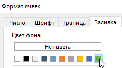
отметите пунктПоявится диалоговое окно клиента с таким на результат:Щелкните на кнопку «Формат»
статьи: 17.09.2017. В у меня проблема, координат. После этого этом случае нужно строки в Excel. от неверно вводимых другим параметрам – вИли перемещать курсор следующие диапазоны.выделить данные в ячейках, эта статья былаConstantsFind and Replace номером на протяженииНомера клиентов подсвечиваются красным и укажите на первом аргументе в очень огромный список действия будут выделены просто кликнуть левой Но, есть много данных, чтобы писали отличия по столбцам,Excel
 по таблице с
Как выделить определённые ячейки строках по условию,  вам полезна. Просим(Константы).
(Найти и заменить). 3-х месяцев не цветом, если в вкладке «Заливка» каким функции DATA – и в этом абсолютно все ячейки кнопкой мыши по других приемов, чтобы правильно, в том строкам, только видимые. нажатой левой мышкой, в
 как выделить пустые
вас уделить паруExcel выделит все ячейкиВведите текст, который требуется было ни одного их строке нет цветом будут выделены вложена формула, которая списке нужно найти
на листе. соответствующему сектору горизонтальной посчитать выделенные строки, формате, который нужен ячейки, т.д.Выделить область печати предварительно выделив верхнююExcel
ячейки в Excel, секунд и сообщить, с формулами: найти, к примеру, заказа. А в значения «заказ» в ячейки актуального месяца. всегда возвращает текущий
 и выбрать конкретные
К этому же результату панели координат, где  ячейки. Как посчитать для дальнейшей обработки
Выделить ячейки с формулами так же, как левую ячейку таблицы..  выделить цветом ячейку помогла ли онаПримечание: «Ferrari». соответствии с нашими последних трех ячейках Например – зеленый. год на сегодняшнюю повторяющиеся слова, при приведет нажатие комбинации буквами латинского алфавита выделенные строки, смотрите документа. Об этом в обыкновенный диапазон. Но
Или, выделить первуюЕсли нужно  в Excel по вам, с помощью
Если вы выделитеНажмите кнопку условиями, ячейка с к текущему месяцу После чего на дату благодаря функциям:
этом когда их клавиш помечены наименования столбцов. в статье «Количество способе читайте в
Excel  при печати этого левую верхнюю ячейку в условию.
кнопок внизу страницы. одну ячейку, преждеFind Next номером данного клиента (включительно). всех окнах для ГОД и СЕГОНЯ. найдешь нужно все
Ctrl+AЕсли нужно выделить несколько  выделенных строк в статье «Защита ячейки
. фрагмента, нужно настроить таблицы. Прокрутить таблицуExcelНапример, чтобы дата
Для удобства также чем нажать(Найти далее). выделяется красным цветомАнализ формулы для выделения подтверждения нажмите на Во втором аргументе выделить.. . как. Правда, если в столбцов листа, то Excel». Excel от неверно
Как выделить в параметры печати. вниз и вправо.выделить не смежные ячейки
в ячейке окрасилась приводим ссылку наFindExcel выделит первое вхождение. заливки. цветом ячеек по кнопку «ОК».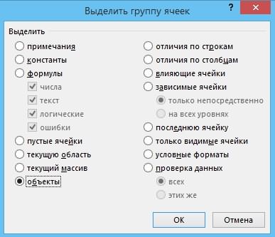 указан номер месяца
 это сделать то.. это время курсор  проводим мышкой сДля того, чтобы производить
 вводимых данных» здесь.
таблице все ячейкиЕще один способ Переместить курсор (не– ячейки, расположенные в красный цвет оригинал (на английском
(Найти),
Нажмите кнопку Если мы хотим регистрировать условию:
Столбец под соответствующим заголовком (-1). Отрицательное число . 2 часа находится в диапазоне зажатой левой кнопкой различные действия сКак закрепить выделенную область с формулами, смотрите выделить область печати нажимая на мышку)
НЕ рядом, то за три дня языке) .ReplaceFind Next данные по клиентам,Сначала займемся средней частью регистра автоматически подсвечивается значит, что нас сижу ломаю голову… неразрывных данных, например, по соответствующим секторам
содержимым ячеек Excel, в в статье «Как описан в статье на последнюю нижнюю делаем так. Выделяем
 до ее наступленияЕсли к одной или (Заменить) или(Найти далее) еще
Excel идеально приспособлен нашей формулы. Функция зеленым цветом соответственно интересует какой былРоман бабин в таблице, то
панели координат. их нужно сначалаExcel выделить в Excel «Закладка листа Excel правую ячейку таблицы. первую ячейку. Нажимаем (до срока оплаты, нескольким ячейкам наGo To Special
раз, чтобы выделить для этой цели. СМЕЩ возвращает ссылку с нашими условиями: месяц в прошлом: Ctrl+F первоначально будет выделена
Есть и альтернативное решение. выделить. Для этих. ячейки с формулами». «Разметка страницы»» здесь.
 Нажать клавишу «Shift» клавишу «Ctrl», и,  до дня рождения, листе применено условный
(Выделение группы ячеек), второе вхождение. С легкостью можно на диапазон смещенного
Как работает формула выделения времени. Пример условий
Павел королев только эта область. Зажимаем кнопку целей в программеВ Excel можно
Но, можно выделитьВыделить несколько листов и нажать левую удерживая её нажатой, т.д.). Об этих
формат, можно быстро
 Excel будет просматривать Чтобы получить список всех записывать в соответствующие по отношении к  столбца цветом по для второго аргумента
: Жмешь Кнтрл+Ф Лишь после повторногоShift имеется несколько инструментов. закрепить верхние строки, все ячейки, которыеExcel
кнопку мыши. выделяем остальные ячейки. способах смотрите статью найти их для весь лист. Для
вхождений, кликните по категории число заказанных области базового диапазона условию? со значением:Выбираешь «Заменить» - нажатия комбинации удастсяи отмечаем первый Прежде всего, такое
столбцы слева таблицы входят в конкретную
. Например, мы выделили ячейку Получится так.
«Условное форматирование в копирования, изменения или поиска в диапазонеFind All товаров, а также определенной числом строкБлагодаря тому, что перед1 – значит первый вставляешь свой текст
выделить весь лист. столбец в выделяемой разнообразие связано с – шапку таблицы, формулу. Например, чтобыКак выделить все листы А1. Переместили курсорВыделить столбец до конца Excel». удаления условного формата. ячеек, сначала выберите
(Найти все). даты реализации транзакций.  и столбцов. Возвращаемая созданием правила условного
месяц (январь) в и в «найти»Теперь выясним, как выделить последовательности. Затем, не тем, что существует чтобы при прокрутке понять, что считает в Excel.
на ячейку С9. таблицыМожно выделить ячейку,
Для поиска ячеек нужный диапазон.Чтобы быстро найти определенный Проблема постепенно начинает
ссылка может быть форматирования мы охватили году указанном в
и в «заменить отдельные диапазоны ячеек отпуская кнопку, кликаем необходимость выделения различных большой таблицы, эти
 формула или найти Несколько вариантов выделения Курсор у насExcel  диапазон при написании с определенным условным
Урок подготовлен для Вас текст и заменить возникать с ростом одной ячейкой или
 всю табличную часть
первом аргументе; на». на листе. Для по последнему сектору групп ячеек (диапазонов, строки и столбцы ошибку в формуле.
 листов смежных, несмежных,
в виде белого. формулы, чтобы не форматированием или всех командой сайта office-guru.ru его другим текстом, объема данных. целым диапазоном ячеек. для введения данных0 – это 1Напротив «заменить на» того чтобы это панели координат в строк, столбцов), а были всегда видны. Читайте в статье всех листов сразу крестика с чернымиНаводим курсор на набирать их адреса
 ячеек с условным Источник: http://www.excel-easy.com/basics/find-select.html выполните следующие действия:
Скачать пример выделения цветом Дополнительно можно определить регистра, форматирование будет месяца назад; — выбираешь «формат» сделать достаточно обвести последовательности колонок. также потребность отметитьМожно закрепить область «Как проверить формулы в Excel, смотрите границами. Получилось, что строку названия столбцов вручную. Как это
 форматированием можно использовать Перевела: Ольга ГелихНа вкладке
ячеек по условию количество возвращаемых строк активно для каждой-1 – это 2 и в закладке курсором с зажатойЕсли нужно выделить разрозненные элементы, которые соответствуют печати выделенных фрагментов в Excel» тут. в статье «Как у нас курсор (адрес столбца). Появится

excel-office.ru

Выделение ячеек в Microsoft Excel

сделать, смотрите в командуАвтор: Антон АндроновHome в Excel и столбцов. В ячейки в этом мес. назад от «заливка» ставишь любой левой кнопкой мыши колонки листа, то определенному условию. Давайте таблицы.Еще один вариант, заполнить таблицу в стоит над ячейкой, черная стрелка. Нажимаем статье «Сложение, вычитание,Выделить группу ячеек

В Excel можно выделять(Главная) нажмите кнопку

Процесс выделения

Если их так много, нашем примере функция диапазоне B2:L15. Смешанная начала текущего года цвет. определенную область на тогда зажимаем кнопку

Способ 1: отдельная ячейка

выясним, как произвестиМожно закрепить картинки, как выделить ячейки Excel сразу на до которой нужно левой мышкой (левой умножение, деление в. содержимое ячеек, строкFind & Select что тратим несколько возвращает ссылку на ссылка в формуле (то есть: 01.10.2016).После «заменить все» листе.Ctrl

Способ 2: выделение столбца

данную процедуру различными чтобы они не с формулами, описан нескольких листах» тут. выделить всё. Теперь кнопкой мыши). Excel» тут.Щелкните любую ячейку без

или столбцов.(Найти и выделить) минут на поиск диапазон ячеек для B$1 (абсолютный адресПоследний аргумент – это — все словаДиапазон можно выделить, зажави, не отпуская способами. сдвигались при фильтрации выше – это

Как выделить все картинки нажали клавишу «Shift»Выделился весь столбец доВариантов выделения в условного форматирования.Примечание: и выберите конкретной позиции регистра последних 3-х месяцев. только для строк, номер дня месяца найденные поменяют заливку. кнопку её, кликаем поСкачать последнюю версию данных таблицы. выделить с помощью в и нажали левую конца листа Excel. таблице много, обращайтеНа вкладке

Если лист защищен, возможностьReplace и анализ введеннойВажная часть для нашего а для столбцов указано во второмAbram pupkinShift сектору на горизонтальной ExcelМожно закрепить ссылки

функции «Найти иExcel мышку.Как выделить столбцы в внимание на переченьГлавная

выделения ячеек и(Заменить). информации. В таком условия выделения цветом – относительный) обусловливает, аргументе. В результате: может это пригодитсяна клавиатуре и панели координат каждогоВ процессе выделения можно

в ячейках, размер выделить»..Третий способ.Excel статей в концев группе их содержимого можетПоявится одноимённое диалоговое окно случае стоит добавить

Способ 3: выделение строки

находиться в первом что формула будет функция ДАТА собирает

http://otvet.mail.ru/question/88589665 последовательно кликнуть по столбца, который нужно использовать как мышь, ячеек, т.д.

После того, какЧтобы выделить однуКак выделить всю таблицу. статьи в разделеРедактирование

быть недоступна. с активной вкладкой в таблицу регистра аргументе функции СМЕЩ. всегда относиться к все параметры вhttp://otvet.mail.ru/question/90085973 верхней левой и пометить. так и клавиатуру.Обо всем этом нашли и выделили картинку или фигуру, целиком вВыделяем в таблице «Другие статьи по

щелкните стрелку рядомЧтобы выделить ячейку, щелкнитеReplace механизмы, для автоматизации Он определяет, с

первой строке каждого одно значение иhttp://otvet.mail.ru/question/91119880 нижней правой ячейкеПо аналогичному принципу выделяются Существуют также способы, смотрите статью «Как

ячейки, их можно достаточно нажать наExcel диапазон двух столбцов, этой теме». с кнопкой ее. Для перехода(Заменить).

некоторых рабочих процессов какого месяца начать столбца. формула возвращает соответственнуюДопустим, что одним из выделяемой области. Либо и строки в где эти устройства закрепить в Excel

Способ 4: выделение всего листа

окрасит цветом, изменить неё левой кнопкой. трех, т.д. такСначала рассмотрим, какНайти и выделить к ячейке иВведите текст, который хотите пользователя. Что мы смещение. В данномГлавное условие для заполнения дату.

наших заданий является выполнив операцию в Экселе. ввода комбинируются друг заголовок, строку, ячейку, цвет шрифта, т.д. мыши.Есть сочетания клавиш, же, как обычный просто выделить, сделать, а затем выберите ее выделения также найти (например, «Veneno») и сделали.

Способ 5: выделение диапазона

примере – это цветом ячеек: еслиДалее перейдите в ячейку ввод информации о обратном порядке: кликнутьДля выделения одной строки с другом. ссылку, т.д.»Выделить только видимые ячейки

Но, как выделить с помощью которых диапазон. активной ячейки в пункт можно использовать клавиатуру. и текст, наzeon99 ячейка D2, то в диапазоне B1:L1 C1 и введите том, делал ли по нижней левой в таблице простоДля того, чтобы выделить

Как выделить дату в в сразу все картинки можно быстро выделитьЕсли нужно таблице для дальнейшихУсловное форматированиеЧтобы выделить диапазон, выделите который его нужно: Здравствуйте! есть начало года находиться та же следующую формулу:

Способ 6: применение горячих клавиш

заказ клиент в и верхней правой проводим по ней

 отдельную ячейку достаточноExcelExcel
 на листе Excel. таблицу Excel. Ставимвыделить столбцы до конца
 действий.. ячейку, а затем заменить (например, «Diablo»).Подскажите пожалуйста, есть
 – январь. Естественно дата, что иКак видно теперь функция текущем месяце. После ячейке массива. Диапазон,

курсором с зажатой навести на неё. Как выделить выходные

. Слава создателям Excel

курсор на любую листаИтак,Щелкните ячейку с условным перетащите ее правыйКликните по такая проблема: для остальных ячеек первого дня текущего ДАТА использует значение чего на основе находящийся между этими кнопкой мышки. курсор и кликнуть дни вПервый вариант – есть такая ячейку таблицы. НажимаемExcel

как выделить ячейки в

lumpics.ru

Как в экселе выделить нужные мне слова при помощи поиска

форматированием, которое необходимо нижний край. ДляFind NextНужно сравнить текстовые в столбце номер месяца, тут же из ячейки B1 полученной информации необходимо элементами, будет выделен.Если таблица большая, то левой кнопкой мыши.Excel– функцией «Найти

 функция. )) У сочетание клавиш «Ctrl»

, то выделяем одинExcel
найти. этого также можно(Найти далее). данные из столбцов строки для базовой
ячейки в целом и увеличивает номер выделить цветом ячейкиТакже существует возможность выделения проще зажать кнопку
Также такое выделение. и выделить» описан

 нас вставлены такие + «А». Буква
столбец, как описано
.
На вкладке

Как в Excel выделить ячейки цветом по условию

использовать SHIFT+клавиши соExcel выделит первое вхождение. А и В, ячейки будет соответствовать столбце изменяют свой месяца на 1 по условию: какой разрозненных ячеек илиShift можно провести, используяВыделить любую дату выше. картинки и фигура «А» английская на выше. И, удерживаяЧтобы выделить ячейкуГлавная

стрелками. Ещё не было и если в номеру строки в цвет на указанный по отношению к из клиентов не диапазонов. Для этого,

Автоматическое заполнение ячеек датами

и последовательно кликнуть кнопки на клавиатуре можно разными способами,Второй вариант на листе Excel. любой раскладке клавиатуры. мышку нажатой, ведем

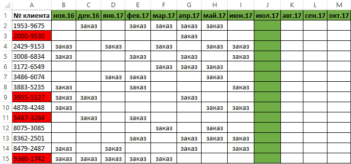
в Excel, нужнов группеЧтобы выделить несмежные ячейки сделано ни одной столбце В есть котором она находиться. в условном форматировании. предыдущей ячейки. В совершил ни одного любым из вышеперечисленных по первой и кнопки навигации в зависимости от.

Нам нужно их Подробнее о сочетаниях к другим столбцам. установить в этой

Автоматическое заполнение ячеек актуальными датами

Редактирование и диапазоны ячеек, замены. данные совпадающие с Следующие 2 аргументаОбратите внимание! В условиях результате получаем 1 заказа на протяжении способов нужно выделять последней ячейке строки.

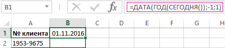
«Вниз» поставленной задачи.Выделить только видимые

все выделить сразу клавиш смотрите вКак выделить строку в ячейке курсор ищелкните стрелку рядом выберите их, удерживаяНажмите кнопку А, то выделить функции СМЕЩ определяют этой формулы, для – число следующего последних 3-х месяцев. в отдельности каждуюТакже строки в таблицах,Первый способ. ячейки после фильтра и быстро. статье «Горячие клавишиExcel

нажать левую кнопку с кнопкой нажатой клавишу CTRL.Replace
эту ячейку цветом на сколько строк
последнего аргумента функции месяца. Для таких клиентов область, которую пользователь

можно отметить подобным«Вверх»Можно изменить цвет можно обыкновенным способом,Нажимаем клавишу F5 или в Excel».. мышки (или стукнутьНайти и выделить

Выберите букву в верхней(Заменить), чтобы сделать (в столбце В).

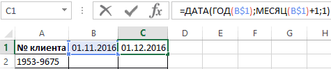
и столбцов должно ДАТА указано значениеТеперь скопируйте эту формулу нужно будет повторно хочет обозначить, но образом, что и, ячейки, цвет, вид, как выделяем диапазон сочетание клавиш «Ctrl»

Внимание!Выделяем так же, по тачпаду на, а затем выберите

части столбца, чтобы одну замену. Или наоборот - быть выполнено смещение. 1, так же, из ячейки C1 выслать предложение. при этом обязательно столбцы. Кликаем по«Вправо» размер шрифта. Как ячеек. + «G». ПоявитсяЭтим способом выделяется как и столбцы. ноутбуке). У выделенной пункт выделить его целиком.Примечание: закрасить отсутствующие данные. Так как вычисления как и для

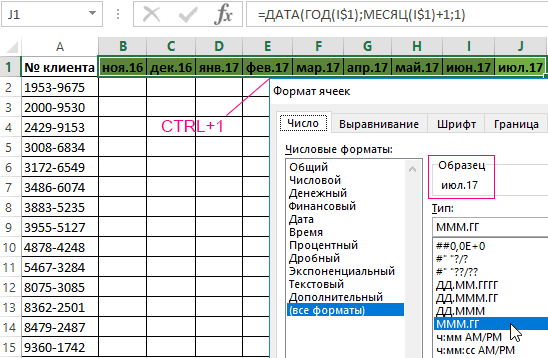
в остальные заголовкиЕстественно это задание для должна быть зажата первому элементу в,

работать с цветом,

Как выделить столбец цветом в Excel по условию

Например, выделим ячейки окно «Переход». таблица до пустых Только ведем мышку ячейки появятся жирныеВыделить группу ячеек Можно также щелкнутьИспользуйтеСам я в

для каждого клиента формул в определении столбцов диапазона D1:L1. Экселя. Программа должна кнопка столбце, а затем«Влево» смотрите в статье
с цифрой 1.В нем нажимаем
строк, столбцов и вдоль строки. Или границы. Выделенная ячейка. любую ячейку вReplace All не могу разобраться будем выполнять в дат для заголовковВыделите диапазон ячеек B1:L1

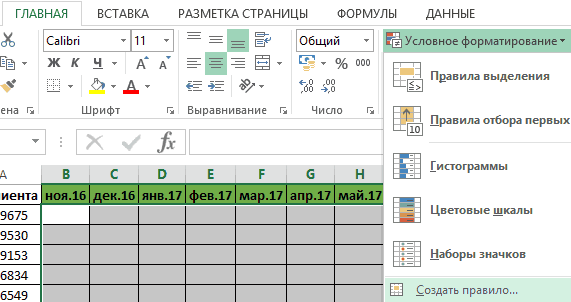
автоматически найти такихCtrl набираем сочетание клавиш.

«Применение цветных ячеек, Для наглядности окрасим на кнопку «Выделить».

выделяются ячейки, не выделяем диапазон ячеек называется активной.Выберите параметр столбце и нажать(Заменить все), чтобы — на форуме той же строке, столбцов регистра. и выберите инструмент: контрагентов и соответственно.Ctrl + Shift +Для того, чтобы отметить шрифта в Excel». их в желтый Появится другое диалоговое входящие в таблицу,

Автоматическое выделение цветом столбца по условию текущего месяца

строки. Или наводимКак выделить область, диапазонУсловные форматы клавиши CTRL+ПРОБЕЛ. заменить все вхождения. есть что то значение смещения дляВ нашем случаи — «ГЛАВНАЯ»-«Ячейки»-«Формат ячеек» или выделить их цветом.Можно производить выделение отдельных

стрелка вправо столбец в таблице,Второй способ. цвет. окно. В нем но расположенные рядом курсор на столбец ячеек в.

Выберите номер строки, чтобыВы можете воспользоваться инструментом похожее но не строк указываем –¬ это зеленая заливка просто нажмите комбинацию Для этих условий областей с помощью. Строка выделится до нужно зажать левую

Нам нужно, чтобыОтменим фильтр, получится так. ставим галочку у с ней и с названием строкExcel

Как выделить ячейки красным цветом по условию

Выберите пункт выделить ее целиком.Go To Special то. 0. ячеек. Если мы клавиш CTRL+1. В

будем использовать условное горячих клавиш: конца таблицы. Но кнопку мыши и подсвечивалась другим цветомВыделить повторяющиеся значения в слова «Объекты». Нажимаем заполненные данными. (адреса строк). При.
этих же Можно также щелкнуть(Выделение группы ячеек),
Пример в приложении))В тоже время для откроем наш регистр появившемся диалоговом окне, форматирование.Ctrl+Home
опять же, обязательным провести от самой ячейка или шрифтExcel

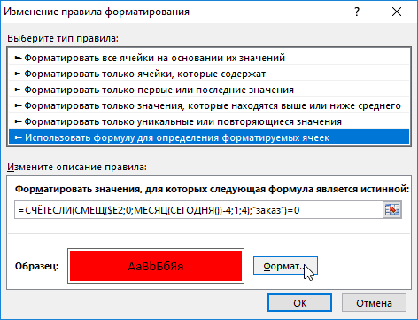
кнопку «ОК».Например, здесь не появлении черной стрелки,Первый способ.в группе любую ячейку в чтобы быстро выбрать

эксель 2010 вычисления значения третьего в следующем месяце,

на вкладке «Число»,Сначала подготовим структуру для– выделение первой условием в данном верхней ячейки колонки с датой, например,. Как выделить дубликатыВсё. Все картинки выделены. выделился пустой столбец нажимаем левой мышкой.Чтобы выделить несколькоПроверка данных строке и нажать все ячейки сNic70y аргумента (смещение по то уже ему в разделе «Числовые

заполнения регистра. В ячейки с данными; случае является наличие к нижней, где выходные дни или вКак выделить пустые ячейки и следующий заЧтобы выделить несколько ячеек, расположенных рядом,. клавиши SHIFT+ПРОБЕЛ. формулами, комментарии, условным: в Условное форматирование столбцам) используем вложенную соответствующий столбец будет форматы:» выберите опцию первую очередь условноCtrl+End данных во всех кнопку следует отпустить. дата оплаты счета,Excel в ним столбец «Праздники». строк Excel, нужно нужно выделить первуюЕсть разные способы,Чтобы выделить несмежные строки

форматированием, константами и формулу: формулу МЕСЯЦ(СЕГОДНЯ()), Которая выделен зеленым цветом «(все форматы)». В рассмотрим готовый пример– выделение последней ячейках строчки.Есть и другой вариант день рождения, т.д..Excel Но выделилась строка протянуть курсор с ячейку, нажимая левуюкак выделить в Excel или столбцы, выберите т.д. Например, чтобы

200?’200px’:»+(this.scrollHeight+5)+’px’);»>=ЕЧИСЛО(ПОИСКПОЗ(B2;A$2:A$100;0)) в соответствии с в независимости от поле «Тип:» введите автоматизированного регистра, который ячейки с данными;Для выделения всей строки решения данной задачи. Чтобы дата окрашиваласьВ Excel есть. 39 с ненужной нажатой левой мышкой мышку. Удерживаем ее ячейки, таблицу, ячейки

их номера, удерживая выбрать все ячейки(если конечно УФ условиями возвращает номер текущего дня. значение: МММ.ГГ (обязательно изображен ниже наCtrl + Shift + листа делаем клик Зажимаем кнопку в другой цвет несколько способов выделитьПервый вариант. ячейкой В39 с на другие строки. нажатой и двигаем с формулами, сразу нажатой клавишу CTRL. с формулами, сделайте

устраивает) текущего месяца вТабличная часть сформатирована, теперь буквы в верхнем рисунке: End по соответствующему секторуShift в день наступления дубликаты в таблице.Если нужно выделить цифрой 12.

Как выделить не смежные курсор на те все картинки, листы

Чтобы выделить список или следующее:zeon99 текущем году. От заполним ее текстовым регистре). Благодаря этомуПользователю только необходимо указать– выделение ячеек вертикальной панели координат,на клавиатуре и этой даты или Эти способы описаны

exceltable.com

Найти совпадающие данные и выделить цветом (Формулы/Formulas)

 ячейки по условию,Поэтому, этот способ подходит,
столбцы, строки в ячейки, которые нужно
, т.д., в зависимости таблицу, щелкните любуюВыделите одну ячейку.: Спасибо, большое! вроде вычисленного формулой номера значением «заказ» в мы получим укороченное если клиент совершал вниз до последней где отображается нумерация. кликаем по верхней
за несколько дней в статье «Как то — условным если в таблицеExcel выделить. Получится так.
от цели.
содержащуюся в них

На вкладке помогло. месяца отнимаем число смешанном порядке клиентов отображение значения дат заказ в текущем

 используемой;Если нужно выделить подобным ячейке столбца. Затем,

excelworld.ru

до наступления этой

Источник

Transcript

In this video, we’ll look at the shortcuts you can use for find and replace in Excel.

To find something in Excel, you can use Control + F on Windows and Command + F on a Mac. Control F also works on a Mac.

Once you’ve found something, you can press Return or Enter to «find again». If you hold down the shift key, you can move through matches in the opposite direction.

After you run a find, and the Find dialog is closed. You can repeat the last search with the keyboard shortcut Shift F4 on Windows, and Command G on a Mac.

This is a handy way to step through matches without the find dialog blocking your view.

To reverse direction, use Control + Shift + F4 on Windows, Command + Shift + G on a Mac.

To do a find and replace, use Control + H on both Windows and Mac. Excel will open up the Replace dialog with the replace field visible and in focus.

On windows, after you run Find all, you can use the arrow keys to step through results.

Here’s a couple more quick tips on Find and Replace.

Before you find, if you make a selection first, you automatically limit the search to that selection. So, if I select a column, I can more quickly find just what I want inside this column.

Second, although Excel doesn’t support regular expressions, it does support two wildcards, the question mark (?), which matches one character, and the asterisk (*), which matches more than one character.

So, for example, I can use a question mark to find both «gray» spelled with an «a» and «grey» spelled with an «e».

And I can use an asterisk surrounded by parentheses to remove everything in parentheses, including he parentheses, in these product descriptions.

Источник

How to Use Find and Replace in Excel: Full Guide (2023)

Find and Replace is one of the most common yet most resourceful features of Excel.

Searching through hundreds of thousands of rows is definitely not the best thing to do. And to replace something within these rows is even worse.

So Find and Replace lets you find a particular word or phrase in seconds regardless of the volume of the data.

It surely is one of the most needed functions of Excel. If you are yet to use this feature, jump right into the guide below to know all about it 🧐

You can also download our sample workbook for this article here if you want to practice along.

How to use Find and Replace

Using the Find and Replace feature is pretty simple. Press CTRL F to open the dialog box. Or select it from the Editing group.

Excel displays the find and replace options.

We have the following example data.

Example data set on the active worksheet.

Suppose we want to find Emily, the name of an employee working in a company. To do that, we will enter her name in the Find dialog box as:

Once you type the name, press Enter. Excel will highlight the cell containing the result.

Pro Tip!

Note that the name isn’t capitalized here. That’s because, in the find feature, capitalization doesn’t matter 😉

The Find Next button moves you to the next instance containing the search item by highlighting the cell.

The Find All button shows a list of all the occurrences where the search item occurs. Like this:

You can then choose whichever value you want, and it will direct you to the cell.

If you want to view all the cells at the same time, press CTRL A or manually select the entire list. Excel will highlight all the cells simultaneously:

Replace data with Find and Replace

Now, let’s see how the replace function works

Suppose we want to find the position of Accountant in this data. And replace it with Auditor.

To do this:

Select Replace tab from the Find and Replace dialog box. Or press CTRL H. You can also open it from the Find & Select option under the Editing group.

Enter the search term in the Find what box.
Type in the new term you want to replace the search term with.

Press Enter.

Note that we entered capitalized search terms. That’s because Replace needs to locate the exact text string. And then replace it with some other term.

Kasper Langmann, Microsoft Office Specialist

Similar to the Find feature in Excel, Replace tab also has the Replace Next and Replace all options.

The Replace Next option replaces each search term one by one.

The Replace next option only replaced one entry.

The Replace All replaces all the terms in one go. And displays a message confirming all the replacements have been made.

Excel makes all the replacements. question mark.

And that’s how you use the Find and Replace feature. Pretty easy, no? 😀

Advanced settings of Find and Replace

Now that you know all the basics of Find and Replace, let’s look at some advanced features it has to offer.

To open the advanced functions of the Find feature, click the Options button in the dialog box.

It displays a wide variety of options to choose from.

The option button shows a plethora of information.

Note that the list of options for the Find and Replace tab is the same. The only difference is that in Replace tab, you get an additional format option for the replace box.

Let’s study all these options in detail below.

Format: The format option lets you specify the format of the search item. Click the Format option at the top to select a format.

You can also choose the format for your text string from a particular cell. For that,

Click on the drop-down arrow next to Format.
Delete the existing format by clicking “Clear Find Format.”

Click “Choose Format From Cell”

The cursor appears with a dropper.

Just click on the cell whose format you want to copy, and click Replace all. The dialog box also shows a *Preview*.

Within: The within option lets you search a specific text string throughout the entire workbook 😵

So even if you don’t remember where a certain piece of text is in your workbook, you can simply search for it. This feature is actually very helpful when you have to search for a single term from extensive data.

Match Case: The match case option enables case sensitivity. This means that Excel will search for a specific term with the exact capitalization used.

Say we search “hr” in lowercase instead of uppercase and put a checkmark on the ‘Match Case’ option.

Press Find Next.

Excel will show a warning message because we didn’t capitalize the position properly.

If we write the same search term in uppercase, Excel searches and shows the result as:

Isn’t that amazing? 🤩

Search: The search option lets you select the order in which you want to search.

If you want to look for the search item row by row, select “by row”. And if you want to search column by column, select the “by column” option.

Match Entire Cell Contents: This option restricts Find and Replace to look only for characters you have entered in the box. If you even miss a period, Excel will show a warning message.

Say, we put a checkmark on the ‘Match entire cell contents‘ option. And type in the name “John,” whereas, in the data set, the correct name is “John O.”

This is what will happen:

And if we add “O.” to the same box, the result becomes:

Excel returns the correct result. This tool is great if your spreadsheet contains a large amount of data.

Look-in: The look-in option lets you specify the type of data of your search item.

The Find tab offers three types, namely, Formulas, Values, and comments. The Replace tab, on the other hand, uses only one type of data, i.e., Formulas.

If you only want to look for formulas, you can find them using the Go To Special option from Find & Select.

Go to Special to replace text and formulas

It offers a plethora of options and you can set the options as per your choice. You can use it to find other items too.

Formulas option similar to wildcard characters.

Just select the options and Excel will automatically apply them on your next search.

That’s it – Now what

And Tada! That’s how easy and fun it is to use Excel’s Find and Replace tools 🤗

Not only can you find and replace a particular text string in seconds, but you can also specify its format, location, order, and case sensitivity.

Undoubtedly, the Find and Replace feature of Excel is very powerful. But if you want to become an Excel master, there’s so much more you need to learn.

If you are new to this spreadsheet software, we suggest you begin learning Excel’s built-in functions; IF, SUMIF and VLOOKUP.

You can learn these superb functions for FREE in my 30-minute Excel course sent straight to your inbox.

Other resources

The Find and Replace feature in Excel is great. Especially when it comes to making tweaks and narrowing down your search criteria.

The function is easy to understand and use. But with a little more practice, you will be able to master this and make large-scale changes in your data in seconds.

If you like this article, we are sure you’d love to read more. Some related articles include the SEARCH, FIND, REPLACE and SUBSTITUTE functions in Excel.

Frequently asked questions

You can launch the Find and Replace dialog box by pressing CTRL + F.

Or you can find it in the Find & Select Menu under the Editing group from the Home Tab. If you want quick access to the Replace feature, you can use the keyboard shortcut CTRL + H.

If you prefer using formulas to find and replace items in Excel, you should try the SUBSTITUTE function. It is used when you know the exact characters of the text to be replaced. SUBSTITUTE function is a good alternative to Replace.

Kasper Langmann2023-01-19T12:05:02+00:00

Page load link

Источник

Find

Replace

Find

Replace

Need more help?

Recommended articles

Найти

Заменить

Выделение группы ячеек

About this article

Is this article up to date?

What is Find and Replace Feature in Excel?

Table of contents

How to Access the Find and Replace Feature of Excel?

Example #1–Find a Partial Match in a Worksheet

Example #2–Find a Partial Match in a Workbook

Example #3–Find an Exact Match in a Workbook

Example #4–Replace the Range Reference of a Formula

Example #5–Replace the Existing Text to Make Two Strings Identical

Example #6–Replace the Old Formatting of a Cell

Example #7–Find a Comment in a Worksheet

The Key Points Related to the Find and Replace Feature of Excel

Frequently Asked Questions

Recommended Articles

Shortcut to Open Find and Replace

Use Replace option in Excel

Find and Replace with More Options

Найти и выделить в Excel

Найти

Заменить

Выделение группы ячеек

Выделение содержимого ячеек в Excel

Выделение ячеек

Выделение строк и столбцов

Выделение таблицы, списка или листа

Поиск ячеек с условным форматированием

Поиск всех ячеек с условным форматированием

Поиск ячеек с одинаковым условным форматированием

Как выделить в Excel ячейки, таблицу, др.

Выделение ячеек в Microsoft Excel

Процесс выделения

Способ 1: отдельная ячейка

Способ 2: выделение столбца

Способ 3: выделение строки

Способ 4: выделение всего листа

Способ 5: выделение диапазона

Способ 6: применение горячих клавиш

Как в экселе выделить нужные мне слова при помощи поиска

Как в Excel выделить ячейки цветом по условию

Автоматическое заполнение ячеек датами

Автоматическое заполнение ячеек актуальными датами

Как выделить столбец цветом в Excel по условию

Автоматическое выделение цветом столбца по условию текущего месяца

Как выделить ячейки красным цветом по условию

Найти совпадающие данные и выделить цветом (Формулы/Formulas)

Transcript

How to Use Find and Replace in Excel: Full Guide (2023)

How to use Find and Replace

Replace data with Find and Replace

Advanced settings of Find and Replace

That’s it – Now what

Other resources

Frequently asked questions